A Complete Analysis of the New Hyper-thin Sensor for Cartridge Valves Predictive Diagnosis
Massimiliano Ruggeri1,*, Francesco Maita2, Luca Maiolo2, Ivano Lucarini2, Mattia Ferri3, Christopher Rosi4, Chiara Gialluca4 and Sara Baldoni4
1STEMS-CNR, via canal bianco 28, 44124 Ferrara, Italy
2IMM-CNR, Via del Fosso del Cavaliere 100, 00133 Roma, Italy
3E.S.T.E. S.r.l., via Francesco Luigi Ferrari 34/2, 44122 Ferrara, Italy
4VIS Hydraulics S.r.l. Innovation Center Via G. Marconi, 115, 41028 Serramazzoni (MO), Italy
E-mail: massimiliano.ruggeri@cnr.it
*Corresponding Author
Received 15 December 2024; Accepted 10 March 2025
Functional Safety asks for diagnose-ability of systems and components in order to check for faults to be recovered in real time to avoid dangerous consequences of the faults themselves. At the same time, new technologies offer new materials and new production processes, which allow the creation of new sensors to meet the requirements of the functional safety certification. In some applications, the diagnosis of failures is not sufficient for safety requirements, because it is necessary to prevent the occurrence of dangerous failures; for that reason predictive diagnosis would be most desirable. Furthermore, diagnostics and predictive diagnosis are not only related to functional safety, but rather to reliability and function availability, which represent two very important aspects of products quality. Cartridge valves are widely used in many hydraulic systems, both in mobile and in industrial applications, and they are often part of systems that must meet high performance level functional safety requirements. Currently available sensors do not contain information on the state of health of the valve itself and its state with respect to the average life and the distance from a dangerous failure. Besides, there are few sensors directly embedded in valves, with the consequence that the diagnosis of valve faults often comes from inference of information from indirect sensors. This contribution deals with describing an innovative sensor and its ability to detect valve failures before they can occur, even with a reasonable time in advance of the moment in which the fault occurs. These hyper-thin strain gauges sensors fit the valve pole tube and their thickness allows installing them between valve body and coil. The innovation is described and both mechanical, electromagnetic, fabrication, signal conditioning and installation aspects are addressed. Burst and Endurance tests on prototypes are shown to demonstrate the efficacy of sensors for valve condition monitoring.
Keywords: Cartridge valve, fatigue breakage, pole tube, strain gauge, valve coil.
In many electro-hydraulic applications nowadays, sensors are placed in manifolds and along the hydraulic circuits, as well as in pumps and motors, in order to acquire data useful for closed loop controls. As very well described in [1], the sensing technology has grown in the years in parallel to control techniques and, in recent years, in parallel with the need for health status of hydraulic components and, in special way, for the health information of valves.
Searching for special sensors “in valves”, it is hard to find anything new, while it is very interesting to learn how much research has been done trying to deduce the health status or simply the status of valves using different inference techniques. Most of these techniques are using remote sensors and data collected from the effects of the valve status in the hydraulic circuit.
The reliability of hydraulic components it is a very heartfelt topic, but in many papers like in [2] it is treated using traditional pressure sensors, based on traditional strain gauges. In fact, reliability is one of the key topics of safety, but safety is also related to faults and to be aware of faults, the component must be observable. Therefore, sensors are necessary for safety reasons, as it is demonstrated in [3], where traditional sensors placed in the hydraulic circuit are used to evaluate the valve faults in an independent metering system. Many different strategies have been developed to try to evaluate the health status of hydraulic components and, in particular, of valves, due to the difficulty of integrating sensors for a direct acquisition of the health status of the valve itself. In [4] authors propose a multi stage diagnosis based on sensor fusion, using accelerometers to analyse the vibration of the hydraulic directional valves. Even in this case, a direct acquisition of the status of the spool or of the health status of the valve is inferred using external and indirect sensors, i.e. sensors not acquiring the primary physical parameter responsible for the information to be collected. In [5] the importance of a real-time, accurate fault detection and isolation system is described for mobile hydraulic valves, and an inference method is proposed, using traditional pressure sensors and a reduced order model with adaptive thresholds. In the already cited [1] it is also described how the diagnosis of the valves is increased for the digital hydraulic valves. This is confirmed for example in [6] and [7], where authors propose an identification method for faulty valves recognition, based on combination of pressure measurements made during the normal operation of the machine and a mathematical model describing the flow balance of the hydraulic system, once again using traditional pressure sensors in the hydraulic circuit. The only experiences of integration of new thin sensors are in [8], where strain gauges are used to acquire and evaluate the correct functionality of a hydraulic clamping system, and in [9], where strain gauges are used to measure micro leakages of a hydraulic cylinder using internally installed strain gauges. This last experience is not a solution for the industrial production, but is useful in order to understand the strain gauges applicability even inside hydraulic components. To summarize, in [10] a survey of all sensors both already in the market and under development are described and, among these, the strain gauge technology seems the only one applicable to the problem the research wants to address, which still represents an open issue both in research field and in industry world.
Even if nowadays there are few examples of direct application of strain gauges to hydraulic valves, in principle, in the context of hydraulic valves, strain gauges might be used in the following ways:
1. Load Monitoring: Hydraulic valves often control the flow and pressure of fluids within a hydraulic system. Strain gauges can be applied to critical components of the valve assembly, such as the valve body or actuator, to monitor the loads they experience during operation. This information can be used for condition monitoring and predictive maintenance.
2. Pressure Relief Valve Monitoring: In hydraulic systems where precise pressure control is crucial, strain gauges can be attached to the housing of pressure relief valves. These strain gauges can detect the deformation of the valve body under different pressure conditions. By monitoring these deformations, it is possible to infer the pressure levels and adjust the valve settings accordingly to maintain optimal pressure regulation. This particular use case has been tried with poor results, due to the difficulty of precisely sensing pressure through the component strain, caused by not sufficient sensitivity of strain gauges.
3. Structural Analysis: Strain gauges can be applied to different parts of the hydraulic valves to analyse the structural behaviour under varying operating conditions. This can help to optimize the design for better performance and durability. This use case could be useful for fatigue tests but was applied only in laboratory under testing campaign.
4. Feedback Control: In some advanced hydraulic systems, strain gauges might be used as part of a feedback control loop, to provide real-time data on the performance of the valve. This information can be used to adjust the operation of the valve dynamically for improved efficiency and precision. This use case is normally applied in industrial environment, for example in industrial pressing machines.
Overall, while strain gauges themselves are not typically integrated directly into hydraulic valves, they could play a valuable role in enhancing the performance, reliability, and safety of hydraulic systems when applied strategically to monitor various parameters related to the valves and their operation.
On the other side there are interesting research focused on analysis methods to study, predict and diagnose valve faults and oil leakage due to fatigue, especially in safety critical applications. The thermal mechanical stress of a valve is presented in [11], while the fatigue analysis of a pressure relief valve is studied in [12] and the breakage of a hydraulic valve is investigated in [13]. All these studies aim to correct valve design to reduce the risk of a failure due to fatigue. The problem is particularly critical due to difficulty of sensing the entire valve to diagnose mechanical breakage of the component and avoid dangerous oil loss. This is presented in [14], where a sound methodology is presented to diagnose oil leakage in pressure relief valve.
The cited references give a couple of important information: strain gauge technology and flexible electronics could play an important role in hydraulic components diagnosis, and there are unsolved diagnosis of critical faults in valves due to impossibility of sensing the entire valve bodies. However, there are several problems to solve, in order to create a new type of sensors capable to cover the faults of the valve body. The proposed sensor could represent a new sensitization methodology and technique for valves, applicable to both spool valves and cartridge valves. The main difference from the described experiences, in the case treated in this article, is that the aim of the proposed sensor is to acquire directly the main physical phenomenon responsible for valve pole tube breakages instead of trying to infer the valve health status from indirect variables sensing. The main principle is to acquire the anomalies in the mechanical strain of the pole tube, using the electrical-mechanical properties of the strain gauges and a proper design of the sensors tailored on each valve model, in order to maximize the sensitivity and to adapt perfectly the temperature compensation. The main objective of this work is to present the new sensor design and technology, to describe the coil new design needed to install the sensor, proving their acceptability in terms of valve performance, and to prove the ability of the sensor in capturing the instantaneous and fatigue modes of failures of the valve. In next paragraphs it will be described the sensor and its production technology, the necessary adaptation of the electro-actuated cartridge valves and the practical experiences at test bench for sensor validation.
Among the different improvements implemented in the years in this branch of mechanical sensors, ultra-flexible and ultra-thin strain gauge sensors represent a class of devices with multiple advantages in terms of sensitivity, conformability, costs etc. Indeed, the conventional fabrication of strain gauges often relies on MEMS-based technology, where controlled environments and expensive microfabrication processes are requested, while roll-to-roll and printing techniques together with additive manufacturing can allow tuning production according by the case, thus reducing the costs of these devices [15]. Especially in biomedical applications and robotics, ultra-flexible strain gauge sensors embody a suitable choice, since a wearable device fits well with human body or garments and it can show proper conformability to non-conventional surfaces [16, 17]. Depending by the high sensitivity of these sensors and by the specific range of strain requested, different materials can be implemented from elastic or stretchable substrates to extremely soft polymers (reaching strain 100%) [17]. To tune the conductivity and mechanical properties, nanocomposites usually based on carbon like materials or piezoelectric composites are used [18, 19]. In this way, through percolation among conductive nanoparticles, it is possible to control the changes in conductivity during the sensors operation [20]. Alternatively, very stretchable polymers (e.g. PDMS) filled with metal nanoparticles can still be utilized to manufacture extremely long-range strain gauge sensors [21]. Generally, with the implementation of metal nanoparticles it is also possible to obtain very high gauge factors in specific sensor operation range (up to few thousands) [22].
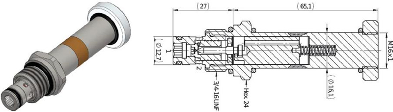
For this research, a proportional Flow regulation Cartridge Valve not pressure compensated, electronically controlled, of VIS Hydraulics was used.
Figure 1 The flow regulation cartridge valve and its section.
The valve is one of the three new valves the company developed in the project, and this one was the first ready for the tests and it is shown in Figure 1, while its characteristic and symbol are shown in Figure 2. The Valve is actuated using a coil of 26 W either 12 or 24 VDC electronically controlled by a new electronic control unit directly connected to the coil connector.
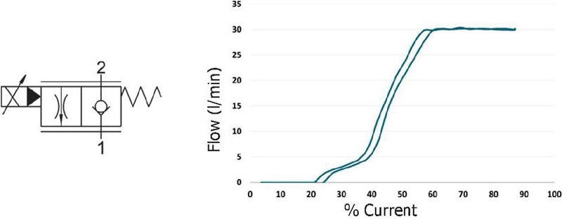
Figure 2 The valve hydraulic symbol and the Current vs Flow characteristic.
There are several breakages of a cartridge valve to be analysed and that can occur during the valve operational life. Different types of breakages can be caused by excessive pressure in operation, which results higher in respect to the maximum pressure declared by the valve producer for the correct usage of the valve itself. Some of them can be caused by fatigue, due to excessive usage of the valve, exceeding the average or declared life of the valve. Others can be caused by mechanical stress, due to external factors or wrong installation of the valve. Finally few of them can be caused by production defects or process defects or material defects. These valve faults can lead to different types of malfunction, the ones we are interested in monitoring are the ones can lead to an oil loss with dangerous consequences, or with function unavailability that can cause damages and high cost consequences. The faults we are discussing of are the faults that can provoke a breakage of the pole tube, whose consequences are shown in Figure 3.
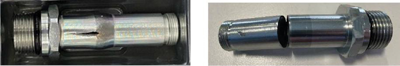
Figure 3 Excessive pressure breakage and process or fatigue breakage of the valve.
The idea developed in this research is to apply sensors to the pole tube, which can directly monitor the health status of the valve. As discussed in the introduction, a sensor type that could fits the requirements, suitable to be installed in between the coil and coil enclosure and the pole tube, is the strain gauge. In fact, any mechanical deformation, or even an oil loss or oil spilling could lead to a sensor deformation and to a variation of the sensor value, then to a recognition of a malfunction of the valve. The different models available have a thickness that is not compatible with the available air gap in the valve. Moreover, it is impossible to find a strain gauge fitting perfectly the envelope of the cylindrical surface of the pole tube. But in the last years the flexible electronics technology had interesting improvements both in materials and in processes, so it is likely possible to design and produce an ad hoc sensor for each valve model. The opportunity of a specific design for each valve model will ensure that any type of breakage of the pole tube will be under the observation area of the sensor. Therefore, theoretically the sensor could reveal any type of breakage during the valve operation life. This is the thesis the research would like to demonstrate. The first step is to understand the sensor technology applied to the sensor prototypes made for this experiment.
The flexible strain gauge sensor has been designed according to a classical meander configuration to obtain a total resistance in the range of [1; 4] kohm. The sensor manufacturing has been performed in a clean room ISO5 to guarantee the standard of fabrication for the devices. It has been exploited thin film technology to manufacture the sensor thus minimizing the waste of materials and it has been used optical lithography to properly miniaturize the devices. To handle the ultra-flexible sensor it has been used a 3 silicon oxidized wafer as carrier depositing over it a polyimide layer (by HD MicroSystems) of 8 m by spin coating. After a thermal treatment at 250C for mechanical stabilization of the polymer, a film of aluminium 150 nm thick has been thermally evaporated. The metal layer has been lithographically patterned with an EVG610 equipment by using a positive photoresist S1813 by Microposit, adopting an ad hoc mask designed with a pattern generator by Heidelberg DWL66.
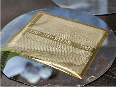
Figure 4 The ultra-thin device after the mechanical release from the wafer. On the left it is possible to see part of the adaptor with the routing for the four sensors.
In this way the resistive sensors with a meander shape working in the range of 1–4 kohm have been created for the different versions of the strain gauge sensor. Finally, to protect the aluminium resistances another layer of polyimide, 2 m thick, has been deposit over the metal, cured at 250C and vias were open to reach out the contacts photolithographically, by using an oxygen plasma treatment with a reactive ion etching machine (RIE) by Oxford Instruments. To protect the aluminium during this process a sacrificial layer of chromium of 25 nm has been evaporated and subsequently removed in an etchant standard solution by Sigma-Aldrich. After this step, the sensor was cut from the wafer and mechanically peeled off, obtaining a thin freestanding device with a total thickness of about 10 m (shown in Figure 4).
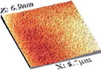
Figure 5 Surface roughness of a spin-coated layer of polyimide measured with an atomic force microscopy technique.
The surface roughness of these devices have been tested to guarantee that the aluminium in the polyimide does not experiment cracks due to the presence of pits or bumps in the polymer, thus compromising the device operation during its lifecycle. As can be observed in the AFM image the typical surface roughness of the polyimide is really low, in the range of few nm: the mean roughness is below 7 nm. (Figure 5).
It is important to highlight that the extremely low surface roughness (lower than 10 nm) guarantees the possibility to deposit thin films (in the range of hundreds of nm) avoiding issues related to surface step coverage that can result in the formation of defects or cracks in the metals. This characteristic is crucial for maintaining the structural integrity and reliability of the strain gauge, thus ensuring a long lifetime of the device
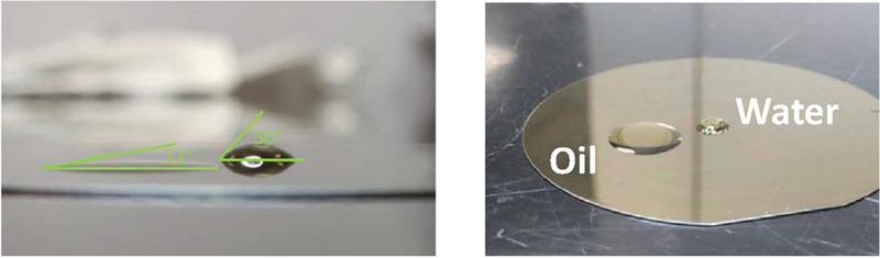
Figure 6 Left figure: the two contact angles for oil and water; right figure: top view of the two drops on polyimide.
To better understand the behavior of fluids on the sensor, the contact angle of water and oil on the polyimide surface has been measured, thus observing the hydrophobicity of the material. Indeed, in case of small leakage it is important to understand how the fluid moves on the device. When a micro-crack opens, some oil drop can be found between the tube and the device. As a function of sensor surface wettability we can obtain different sensors signals. As can be seen in Figure 6, two contact angles for water and motor oil of respectively 50 and 11 have been obtained, so that the wettability of the oil on the polyimide turns out to be really high. The measure of the wettability on the polyimide shows a comparison between oil and water, pointing out that the difference in the contact angles are consistent (11 vs 50). The meaning of this measure is that the sensor surface has a higher capacity in removing water respect oil, offering the ability to discriminate the presence of one liquid respect the other. Since the goal of the sensor is to operate in an environment with possible oil contamination, this difference in wettability can be useful because oil leakage can more easily remain between the sensor and the valve creating an additional strain for the device, while water derived potentially from moisture can be easily removed by vibrations in the system due to its higher hydrophobicity. This difference in wettability can be adjusted, making it even made more significant by modifying the sensor polymer surface with fluorinated agents using a mild treatment in oxygen plasma or CHF3 plasma as explained in [25–27].
Table 1 Sensor Prototypes main characteristics
| Substrate | Metal | Sacrificial | Reference | |
| Prototype | Thickness (m) | Thickness (nm) | Layer (nm) | Resistance |
| 1 | 8 | 120 | none | Yes |
| 2 | 8 | 200 | none | Yes |
| 3 | 12 | 120 | 25 | Yes |
| 4 | 12 | 200 | 25 | Yes |
Different devices were tested with diverse thicknesses of Aluminium, ranging from 120 to 200 nm as shown in Table 1, and a sacrificial layer of chromium 25 nm thick to protect additionally the aluminium film during the manufacturing process was implemented.
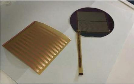
Figure 7 A photograph of the strain gauge with the adaptor.
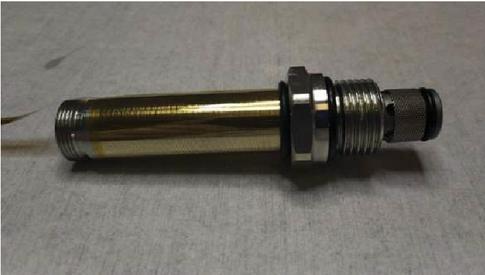
Figure 8 The device wrapped around the valve.
For the first set of tests related to pressure bursts and pole tube deformation, for each device two equal sensors have been fabricated, in order to compensate the temperature variations during the testing procedure. The sensor’s overall dimensions were carefully designed to precisely wrap around the entire pole tube of the cartridge valve selected for testing purposes, ensuring seamless integration and accurate performance evaluation. To facilitate signal extraction, a flexible adapter made from Kapton film with a copper thickness of 12 m was designed, fabricated, and connected to the polyimide substrate using an anisotropic conductive tape, ensuring robust electrical and mechanical bonding (Figure 7). Subsequently, the sensor was securely adhered to the pole tube with glue and conformably wrapped around the valve, ensuring a tight and uniform fit that maximizes surface contact and minimizes the potential for mechanical misalignments (Figure 8). In this way it is possible to monitor valve deformation in each part of the pole tube.
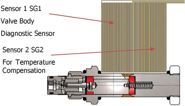
Figure 9 Correspondence between pole tube structure and double sensor design.
The strain gauge sensor obviously reacts to any type of strain, so even to the temperature strain. It is then necessary to create a sensor capable of distinguish between pressure strain and temperature strain, in order to understand the part of the strain due to temperature and the part due to the normal pressure strain, or any abnormal strain, due probably to fatigue or excessive pressure, or pole tube defects. For this reason, a double strain sensor was designed, adapted to the structure of the valve. As shown in Figure 9, it can be noted that part of the pole tube is solid and part is hollow to allow the sliding of the mobile part. Consequently, the first part of the body will change its shape only for temperature, while the second one for both temperature and pressure or fatigue. Hence, the sensor was designed to have one resistance facing to the solid part of the pole tube (SG2), to be used as a reference for temperature strain, and a second resistance to be connected to the hollow part of the pole tube (SG1), sensitive to both pressure and temperature.
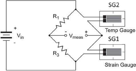
Figure 10 Full bridge configuration.
By a classic full bridge connection in the electronic readout system (Figure 10), it is possible to compensate the strain for temperature in the acquisition of the deformation of the SG1 sensor, subtracting the strain of the SG2 sensor, taking into account in the electronic circuit any difference in resistance of the two sensors, as shown in Equation (1), where is the strain of the sensor in the main direction along the resistive lines.
| (1) |
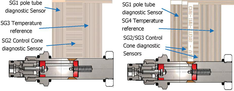
Figure 11 Three and four strain gauges sensor configuration.
In respect to the first experiences with these new sensors presented in [23], where the efficiency of the sensor had been evaluated against deformation and rupture tests against cases of excessive pressure, in [24] other sensor topologies were designed and tested, in order to better evaluate a part of the pole tube that presented some weakness in endurance tests. In fact, as it will be explained in the tests and test results description, endurance tests shown a critical area around the control cone. For that reason a couple of new sensors were designed, to have a more specialized sensor around this area, for an earlier abnormal conditions detection. The sensors architecture are shown in Figure 11. As it can be observed in the figure, the new sensors have the resistive lines in axial direction, while the SG1 and SG4 in the right figure and SG1 and SG3 in the left figure are circumferentially lined up. This fact comes from the Figure 3, where it can be noted that failures due to excessive pressure, result in an axial fracture in the area of SG1 sensor, while the fatigue failures lead to fractures in circumferential direction in the area of SG2 and SG3 as in Figure 3 right. The direction of lines in the new sensors are designed to maximize the strain effect, trying to couple the failure types and their positions with more specialized sensors.
Due to the specific area of the pole tube enveloped by the single sensors, the four sensors topology was preferred. For the hardware readout electronic stage in the control unit design, the single sensor resistive value acquisition can be obtained using again a full bridge topology, but it is necessary to mount different resistive values in the fixed circuit branch of the full bridge, to compensate the difference in resistance values of the SG1, SG2 and SG3 resistances in respect to SG4 resistance, used as temperature reference. The resistive values of SG1, SG2, SG3 and SG4, can also be obtained using four half bridges readout circuitries (an example in Figure 4.12) and calculating the strain by a software function as shown in Equations (2), (3) and (4), with the advantage of reading all sensors values individually, and having a more complete information on the valve health status.
| (2) | |
| (3) | |
| (4) |
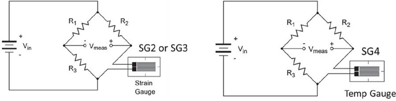
Figure 12 Two half bridge configuration.
In this experience, we used this second approach, due to the need to test different sensors with different characteristic resistances and due to the easiness of correcting temperature strain by software. It will be demonstrated in the tests description that this approach enabled a more complete diagnosis of sensors independently from the gluing method used to install the sensor in the pole tube of the cartridge valve.
Due to the specific design of the sensor, a problem that arose in the feasibility study related to the application of these sensors, was related to their installation on the valve. In particular, the strain gauge is placed above the pole tube, it is glued to the outer part of it, and the solenoid will be placed above the assembly of valve and strain gauge sensor. However, the solenoid enclosure is accurately designed in order to maximize the magnetic flux and part of the design is the minimization of the air gap between the valve coil and the pole tube. Consequently, the thickness of the sensor, although limited, requires a modification of the internal dimensions of the solenoid enclosure, to allow its insertion in between pole tube and coil enclosure. Figure 13 represents a sectional view of the valve and the solenoid. In the figure, a hypothetical magnetization path is highlighted with the dotted red line, which runs through the armature of the solenoid, the fixed core, the moving plunger and control cone.
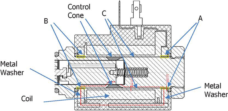
Figure 13 Valve section with air gaps indication.
This Figure 13 shows also the air gaps that are to be redesigned, in order to allow the sensor placement. As it can be noted in red a very reduced air gap of 0,05 mm is available all along the pole tube and the coil (C parts in the figure), while in the two metallic rings at the end of the coil the air gap is 0,1 mm (B and A parts in the figure). The air gaps corresponding to the rings are highlighted in yellow in the figure. Each air gap represents a source of dispersion of magnetic flux that in these positions is not conduct in a magnetic guide. The magnetic flux dispersion ends in a reduced coil force, proportionally. Then, the areas highlighted in yellow represent the air gaps along the path. The connector of the sensor is placed under the metal washer A and it is made of the same material of the sensor, so it also needs a small air gap to be placed in the proper position. The upper side (A part in the figure), where the connector is placed, is not highlighted, nor the empty area on the lower side (B part in the figure), since in reality the armature completely envelops the solenoid. Therefore, those areas are only “punctual” and are seen only in the plane chosen for the section, in the real valve the flow will pass around. Furthermore, the nominal thickness of the gaps between metal washers and tube, and between coil and tube, are shown, to indicate the space available for the sensor. The problem to be addressed in this case concerns the magnetic performance of the assembly, which is influenced by the presence of these air gaps, which introduce real losses. In fact, a circuit analogy can be made and the magnetic path can be represented as a sort of electrical circuit, where the various parts crossed are similar to electrical components. Each source of loss is schematized as a resistance, and all the air gaps encountered (for example the one between the metal washer that makes up the armature of the solenoid) will therefore be resistances that oppose the circulation of “current” that is the analog element of the magnetic flux.
Although the thicknesses involved seems sufficient compared to the thickness of the sensors (we are talking about 25 m in the worst case), it must be considered that the sensor includes a plastic film that encloses the actual sensor, and the output cables. It is therefore necessary to obtain sufficient space for their accommodation, increasing these values. Losses will inevitably be introduced, and this is why a study was conducted using the EMS electromagnetic FEM (EMS, Advanced Electromagnetic Design and Analysis Tool dedicated add-on of the Solidworks suite), to evaluate the impact of any structural modifications to the coil on the electromagnetic performance of the valve. In order to understand how the analysis was performed and how the best configuration was chosen, the various case studies analyzed and the impact they had on the magnetic flux are reported. With reference to Figure 13, it is defined thickness A the thickness of the air gap between the tube and the upper armature of the solenoid (where the sensor connector is placed), thickness B the thickness of the air gap between the tube and the lower armature of the solenoid, while thickness C the thickness of the air gap between the tube and the solenoid, where the whole sensor is placed. The three air gap zones are shown in the figure. In order to define the range of use of the valve and to calculate the absolute stroke in the simulations, we consider the stop between the plunger and fixed core at the position of 4,5 mm stroke, with the valve completely closed at lower stop. Considering a core stroke of approximately 2,75 mm, reaching the mechanical stop in the shuttle part of the valve at 1,75 mm stroke with the valve fully open. This defines the range of use of the valve, since the equilibrium position between the force of the coil and the opposing force of the spring will necessarily be reached in this range of travel. In order to evaluate the worsening due to the modified coil enclosure in the air gaps, the steady state current was analyzed, which defines the “limit” of use in terms of current applicable to the solenoid.
Table 2 Coil air gaps cases for simulation
| Case | Thickness A | Thickness B | Thickness C |
| Standard (Production) | 0.1 mm | 0.1 mm | 0.05 mm |
| A | 0.3 mm | 0.3 mm | 0.3 mm |
| B | 0.4 mm | 0.4 mm | 0.4 mm |
| C | 0.1 mm | 0.4 mm | 0.4 mm |
| D | 0.1 mm | 0.3 mm | 0.3 mm |
| E | 0.45 mm | 0.45 mm | 0.45 mm |
| F | 0.1 mm | 0.45 mm | 0.45 mm |
| G | 0.5 mm | 0.5 mm | 0.5 mm |
| H | 0.1 mm | 0.5 mm | 0.5 mm |
| I (splitted washers) | 0.1 mm | 0.1 mm | 0.05 mm |
Various simulated cases with different air gaps were analyzed from the Electromagnetic point of view, calculating the electromagnetic field intensity, its dispersion and the field density in the area of the plunger movement control, especially near the control cone of the valve. All the analyzed cases are reported in Table 2.
In the first step, the cases ranging from A to H were simulated, in order to find the best combination that allows to install successfully the sensor without compromising the valve functionality in terms of magnetic field and thus magnetic force transmitted to the valve spool. All these cases were simulated, in order to understand the effect of an increased air gap and how the negative effect of the air gap can be reduced, using a washer with minimum air gap in the critical area of the end of the coil. In fact, in this area the magnetic flux is conduct in a magnetic ring through the metal washer, in order to maximize the magnetic flux near the mobile core of the valve and the control cone. For that reason, all cases are shown, to evaluate the dispersion of the magnetic flux and the consequent coil force reduction and to evaluate qualitatively its acceptability in function of valve functionality, energy balance and cost.
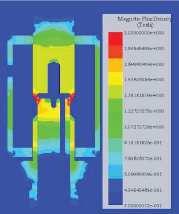
Figure 14 Case A at maximum current.
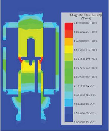
Figure 15 Case B at maximum current.
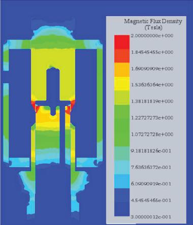
Figure 16 Case C at maximum current.
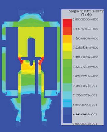
Figure 17 Case D at maximum current.
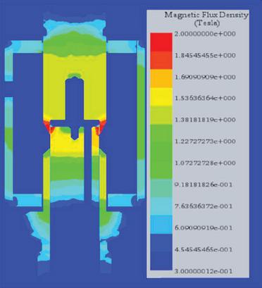
Figure 18 Case E at maximum current.
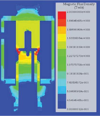
Figure 19 Case F at maximum current.
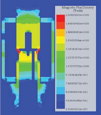
Figure 20 Case G at maximum current.
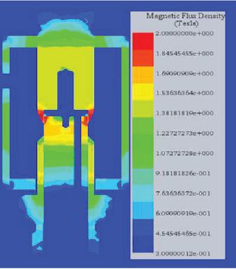
Figure 21 Case H at maximum current.
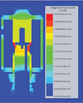
Figure 22 Case I at maximum current.
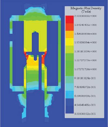
Figure 23 Case Std. at max. current.
From Figures 14 to 23, all simulation cases are shown. It is evident the difference between the standard case, with minimum air gap, and the case G, which can be defined the worst case. As it can be observed, in correspondence of the metal washers, both upper and lower, as referred in Figure 13, the field is interrupted around the coil armature and, consequently, the flux is dispersed. This is due to the larger air gap around coil. The consequence is the reduction of the flux intensity also in the area of the control cone, where the field should be maximum, in order to control the valve plunger position. The yellow color, in respect to the orange available in the standard case, indicates that the field is lower in most of cases. Even in cases where the orange color is visible, the orange area is smaller in respect to standard case. The last consequence is the reduction of the coil force and the impossibility to control properly the valve even at maximum current. The only two cases that seem to be comparable with the standard case are case D (Figure 17) for a “standard” coil and the case I (Figure 22), which is the result of a new study that lead to a new coil composition.
To quantitatively evaluate the magnetic flux force reduction in the cases from case A to case I in respect to the case Standard, a quantitative analysis has been executed. The results are shown in the graphs in figures from Figures 24 to 27, at different values of current circulating in the coil. In the graphs are presented the percentage variations evaluated with respect to standard coil composition, at fixed plunger distances and with coil currents of 0,4 A, 0,8 A, 1,2 A and 1,45 A respectively. This analysis is required because the spool position is obtained through an equilibrium between spring and electromagnetic force, and the maximum admitted electromagnetic force degradation shall be limited, in order to be able to fully open the valve with the available current limits of the coil. A higher current brings to a higher energy consumption and a higher heat generation, thus, as a consequence, to worsening the coil performances at the same valve spool working point. Observing the different case studies, the one that offers the best tradeoff between available space to install the sensor and valve performance with standard coil structure, is the case D, which corresponds to the smallest air gaps and to the smallest change in the upper metal washer in respect to the figures, which allow the mounting of the coil in the pole tube with the sensor glued in its outer surface (0,3 mm for the washers). The case I, the real optimal one, is not considered in this paragraph, due to its different coil composition, which will be discussed later.
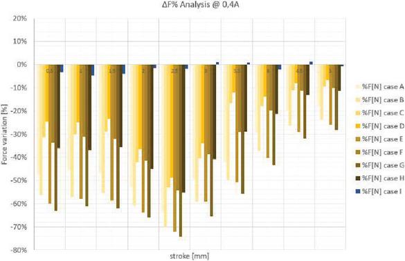
Figure 24 Percentage magnetic field intensity variation @ 0.4A.
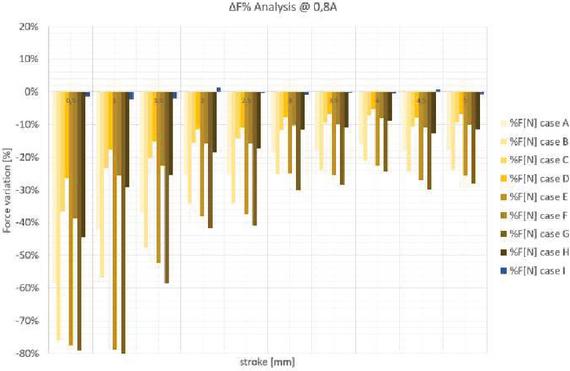
Figure 25 Percentage magnetic field intensity variation @ 0.8A.
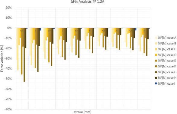
Figure 26 Percentage magnetic field intensity variation @ 1.2A.
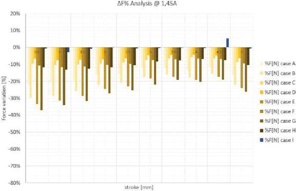
Figure 27 Percentage magnetic field intensity variation @ 1.45A.
In fact in all the graphs presented in the figures, the smallest magnetic flux intensity reduction corresponds to special case I (in blue in the graphs) and, for traditional coil, to case D (the central orange bar in the graphs), even if some other case presents a similar performance.
To justify mathematically these electromagnetic data on the simulations reported on the graphs, the EMWORKS EMS (Electro Mechanical Simulator of Solidworks) method shall be introduced. In particular, EMS solves the Maxwell equations of the electromagnetic interaction. In particular, it solves the two magneto-static analysis Equations (5) and (6) called Gauss’s law for magnetism, which is the most useful for identifying the intensity characteristics of the magnetic field generated in each topology under study.
| (5) | |
| (6) |
The simulator calculates the attraction force F between fixed and moving parts of the valve, using the virtual work method and it calculates the value of the total magnetic energy when an object moves from a position 1 (W) to a position 2 (W) at a Ds distance (Equation 7).
| (7) | |
| (8) | |
| (9) |
In the case of magnetic elements, the Work W is calculated in Equation (8) in the Volume of the elements under study and the reason of the magnetic field flux density reduction, due to the enlargement of the air gaps in the coil cavity, is clear in Equation (9). In this equation, B is the magnetic induction field or magnetic field flux density, H is the magnetic field, v is the volume, is the magnetic air permeability and the is the magnetic permeability of the metal used for the valve ((AVZ) 1.000). It is then clear that, in case of a larger air gaps, the Fs reduced by a smaller value in the factor in the incremental volume of the air gap in respect to the standard case. The magnetic field H does not change, because it depends on number of turns of the coil winding and the current, while B changes due to change of the air gap size.
The analysis justifies the reason why higher currents are needed to control the valve plunger in all cases analyzed other than the Standard one and case I, due to bigger air gaps available in the assembly. Then, in order to reduce as much as possible the deterioration of performance, it is necessary to optimize the air gap. From the analysis of the simulation results, it appears that the optimal case is case D, where it can be noted that metal washer that makes up the ring armor in area A (Figure 13), has the same air gap of the standard case, in order to not disperse the magnetic flux in that area. The case D is the one used for all the real tests on the valve prototypes presented in this research.
For a more complete electromagnetic analysis and also to propose an alternative solution to the worsening of electromagnetic performance, another approach to the coil design was attempted. The lower metal washer shall be enlarged to allow the coil mounting operation over a pole tube preassembled with the sensor. But in the final position of the lower metal washer the sensor is not present. The same applies to the upper metal washer, which has been modified just to allow the positioning of the sensor flat cable to an external connector. For that reason a different approach to metal washer structure and mounting can lead to an optimal coil performance from the electromagnetic flux point of view.
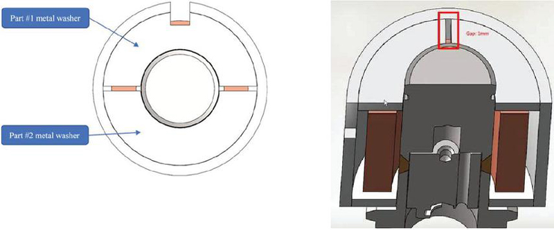
Figure 28 New metal washer design.
A possible further option to improve the installation capabilities is to realize both washers in two pieces as represented in Figure 28. With this coil assembly configuration it is possible in sequence: to mount the sensor over the pole tube, to mount the coil over the assembled pole tube, then to insert the washers, avoiding interference and finally to block the coil and the washers with the final screw. Comparing the magnetic flux intensity in Figure 22 (case I) and Figure 23 (case Std.) the simulation shows that in this case I the performance of the valve is similar to that of the standard case. The Figures underline that to split the washers does not affect the overall armature capability to confine the electromagnetic field, thus the pole tube performance is preserved. This result is obtained starting from the D case, but the same conclusions can be made with the other case studies, obtaining a new degree of freedom in terms of coil installation capabilities. The result of this study is that from the electromagnetic point of view the necessary design modification of the valve assembly don’t affect the valve electromagnetic performance.
Once the coil and coil enclosure air gaps have been defined, the coils have been modified in order to assemble the prototypes. The air gaps have been modified by mechanical tooling enlarging only one ring, with the configuration of the case D. Furthermore two milled flats of the plastic layer in the rear part of the coil were made by mechanical tooling, to allow the housing of the flat cable which brings the poles of the two resistive sensors which make up the strain gauge to the outside (Figure 29 left). This was done to allow the fixing of the nut that holds the coil in place, once placed in the correct position with respect to the spaces available in the manifold, without risking damaging the flat cable itself. The result of the assembly ready to be tested at the test bench is shown in Figure 29 right.
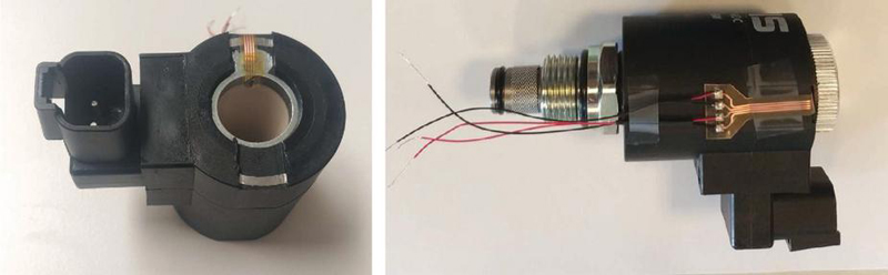
Figure 29 Modified coil with the sensor connector (left) and Valve Assembly (right).
The Valve with the new sensor must be characterized and the expected behaviour is that the sensor should not detect signal variations during valve operation under nominal and healthy conditions, because of the very limited deformation of the valve body expected, while it should detect signal variation, if the valve is subject to higher-pressure levels (250 bar).
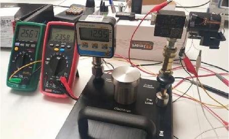
Figure 30 Static pressure test bench.
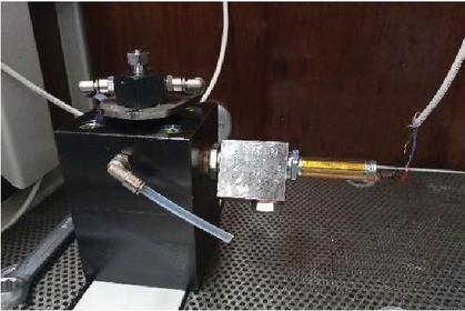
Figure 31 Dynamic pressure test bench.
The first tests have been conducted at the static test bench (Figure 30), increasing the delivery pressure in the valve manually in static conditions through a hydraulic cylinder, in order to characterize the sensor resistances in nominal and ambient temperature conditions. In the range [0; 250] bar a barely detectable change in sensor resistance was observed, confirming that the sensor is not reporting a significant deformation in nominal conditions, exactly as other strain gauges used in past experiences. While the tests at the dynamic pressure bench (Figure 31), used for valve burst tests, made possible to fully characterize sensors in respect to valve deformation. The tests were conducted in two different conditions: valve without coil and valve with coil. In fact, the coil presence changes the fault conditions for the sensor which, due to excessive deformation of the pole tube and the limited air gap, it is crushed between the pole tube and the coil. For that reason, the sensor often breaks in short circuit, resulting in a zero resistance measurement. On the contrary, without coil the more frequent fault for the sensor is case of excessive strain is in open circuit condition.
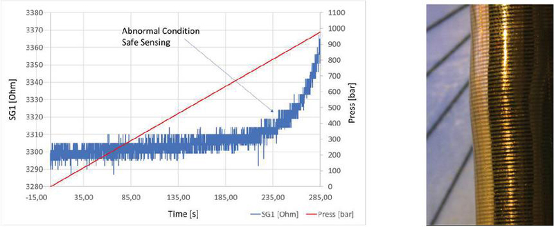
Figure 32 Pressure Transient Test.
The described faults happen at the end of the burst tests or pressure tests, when the valve breaks with a consequent oil loss, or even before that condition if the sensor breaks due to an excessive pole tube deformation.
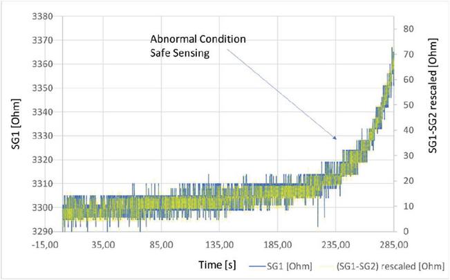
Figure 33 SG1 sensor signal comparison with (SG1-SG2) rescaled and referred to zero.
The described tests were necessary to validate the capability of the sensor of providing a useful signal when in faulty conditions, to detect faults of the sensor itself, because of the valve failure or breakage. However, the tests allowed recognizing abnormal conditions much earlier than valve failure conditions, so sensor breakage represents a limit condition that should rarely be reached in real applications. In fact, a series of tests were conducted stopping the dynamic pressure test bench once the electronic control system was able to recognize a changing signal of the sensor in respect to its base line (Figure 32). As it can be noted in Figure 32, the sensor in nominal working conditions is stable at a constant value, temperature dependent, while when for pressure or yielding of the pole tube, the tube shape changes, then the sensor acquire a signal that differs from the baseline of SG1 more than the 0,5% or 1% (15–30 ).
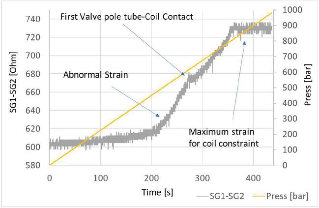
Figure 34 (SG1-SG2) in respect to Bench pressure in the test with Coil.
The Electronic control is equipped with an analogue readout circuit adapted to the resistance of the sensor and with an amplification of the analogue signal, which is also adapted to the specific sensor. In these conditions 70 ohm can represent the 40 or 50% of the entire signal variation captured by the Analog to Digital converter (ADC) dedicated to the SG1 (sensor) input. The SG2 sensor is connected with a similar circuitry, so the resolution can be very high in respect to signal transition. In Figure 33, in fact it is represented how the two signals SG1 and the SG1 referred to the SG2 sensor signal (SG1-SG2), which represents the pure temperature strain, are equivalent in shape and range.
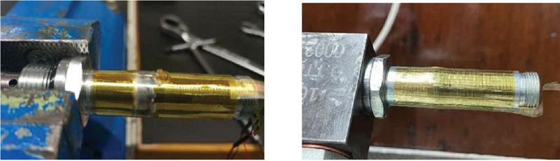
Figure 35 Valve pole tube in case of Coil and no coil.
This consideration leads to prove that both configurations described (full bridge or two half bridges) are equivalent from the signal resolution point of view and are both functional for detecting anomalous deformations of the pole tube. The characterisation of the solution also analyses how the sensor reacts to the deformation in presence of the coil, which is a restraint in the pole tube expansion.
In Figure 34 it is shown a test on the dynamic pressure test bench where the test is stopped before the pole tube damage. In the chart, it is clearly visible the limit for sensor acquired strain that is also the limit of the pole tube enlargement due to small air gap available between pole tube and coil (and plastic coil enclosure). In addition, in this case, the sensor was able to capture the abnormal strain and the limited space did not affect the sensor’s ability to detect an anomalous condition of deformation of the pole tube. Unfortunately, due to the hard contact, it is impossible to analyse the sensor after the test because the tube deformation is inelastic, and pole tube and coil are stuck and the sensor is crushed between the two elements. The described condition is shown in Figure 35, where it is visible the resulting deformation of the pole tube when the coil is extracted using a puller to overcome the resistance caused by the deformed pole tube. As it can be noted the shape of the pole tube deformation it is not rounded as in the case of no coil, so it is limited by coil presence.
In order to validate and to find a correlation between the burst tests and the valve model, FEM analysis have been executed at various pressure levels.
For the simulation conditions it has been assumed that the valve piloting is axialsymmetric, then a bi-dimensional model has been used for the study. The only part of the valve that is not axialsymmetric in fact is the hexagonal area of the valve fixing nut, which however is an area not subject to significant deformations, and it was approximated as a cylindrical section, for which the above assumption was made and a two-dimensional model was used.
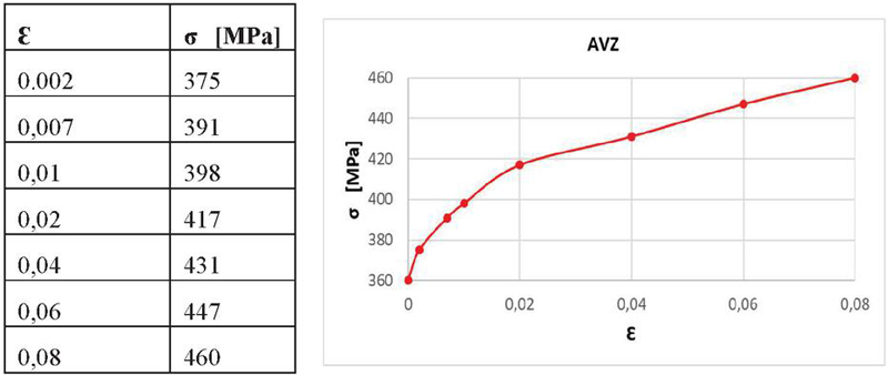
For the material, the parameters of 11SMn30 (AVZ) have been used and for welding-brazing joint the CuAl8 material has been used.
The interactions between the pole tube components of different materials were imposed between: welding joint, HAZ (heat affected zone) and remaining part of the pole tube. To simulate the welding, a union joint was assumed between welding joint and the two HAZ portions of the pole tube; the same was assumed between the two HAZ portions and the remaining pole tube. To fix the component a rigid constraint was imposed to the thread to simulate the insertion of the pole tube into the cavity.
For pressure distribution, the hypothesis of a uniform distribution inside the pole tube was made. FEM simulations were executed at: 250 bar, 400 bar, 500 bar, 600 bar, 750 bar, 900 bar, in order to verify the deformations measured during the test at pressure bench, and to investigate the possible causes of cracks in the material in the different component parts of the pole tube, joined together by mixed welding-brazing process at lower temperature in respect to welding process. The pressure values for the FEMs are not equally spaced, because particular attention was paid to the range of pressure values in which the first perceptible deformations occur, which can be acquired by the new sensors.
Furthermore, the properties of the CuAl8 welding material have been slightly modified, because in reality, by being subject to a brazing process, the resistances of the alloy decrease drastically. In fact, an alteration of the materials is created, identified by the Heat Altered Zone (HAZ) which generally expands beyond the welding part. Also the properties of the AVZ decrease in the thermally altered zone, but having seen both in the experimental cases during the burst tests, and during the simulations that the breakages mainly involved the weld seam, it was decided to focus only on that material. Therefore, the mechanical properties from the technical data sheet were not used, instead a - diagram relating to CuAl8 alloy was identified, which replicated the real degradation conditions following a hot forging production process. This in fact presupposes that a degradation of the mechanical properties occurs connected to the application of heat (in the case under study it would be brazing) which generates residual stresses due to heating/cooling. This leads to lower mechanical properties both for the welding material and in the first 10 mm of interface between welding and base material (but for a more conservative study this interface was expanded to 20–30 mm), after which the metal returns having the mechanical properties of the piloting, as per the technical data sheet, as shown in Figure 36.
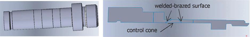
Figure 36 3D Model and axialsymmetric model of pole tube in study with CuAl8 welding and 20-30mm of HAZ of offset up and down.
Therefore, a yield diagram it has been assumed, that was intermediate between the - curve at 650C and 700C of the forged CuAl8 by inserting the points in Table 3.
Table 3 Yield Diagram of the forged CuAl8 at an average temperature between 650C and 700C
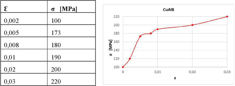
In Table 3 the elastic modulus E=50 GPa is derived both from table and from diagram.
This choice was made because this diagram is the one closest to the experimental strain of the pole tube acquired during the real tests at pressure test bench during the burst tests.
The yield diagram of AVZ material is already known from experimental calculations of material characterization and inserting the points in Table 4.
Table 4 Yield Diagram of the AVZ at an average temperature between 650C and 700C
A triangular mesh is used for the FEM simulation (Figure 37). To guarantee the correct transmission of deformations between the weld bead, the HAZ and the remaining pole tube, the following conditions were applied to the mesh: between the weld bead and the HAZ the common nodes were positioned on the contact boundary line between the components with nodes on the surface; between the HAZ and the remaining pole tube the mesh is kept independent but always with nodes on the surface. This because we wanted to keep a greater mesh density in the areas most subject to deformation the welding bead and HAZ, while in the remaining pole tube the mesh is coarser. Mesh controls were applied to refine it in the most interesting points such as the internal fillets, the weld bead and the HAZ.
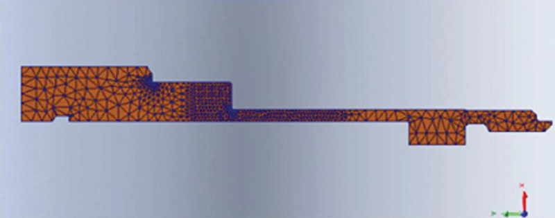
Figure 37 Pole tube mesh.
At the internal connections the maximum size of the side of the mesh triangle is 0.07 mm with an element ratio of 1/4; at the weld bead and HAZ the maximum size of the mesh triangle bed is 0.5 mm with the same ratio 1/4. While in the remaining pole tube a standard mesh is kept coarser, with a maximum triangle side size of 1.5 mm. The total number of triangular elements by which the axial symmetric section of the tube pole has been subdivided by the simulator is 1089 elements. As shown in the Figure 37, the regions that distinguish the welded part and the HAZ areas from the rest of the pole tube are generated with more refined component elements.
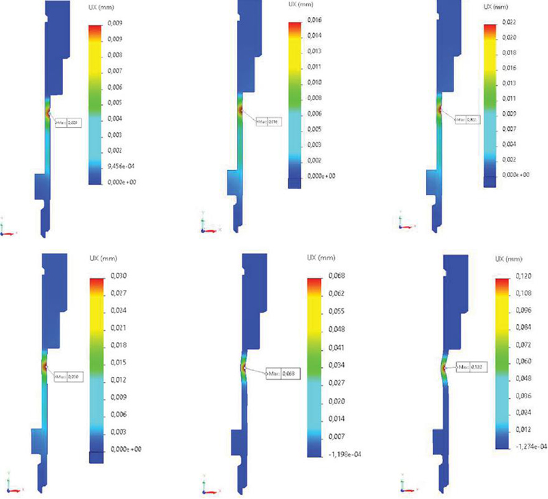
Figure 38 Strain in FEM at 250 bar (top left), 400 bar (top center), 500 bar (top right), 600 bar (down left), 725 bar (down center) and 900 bar (down right) of internal pressure.
Some of the FEM Analysis results are presented in Figure 38. Six FEM results at pressure values from minimum to high pressure in relation to the pressure range of the burst test are presented. The FEM results are coherent with experimental tests and FEM highlights that in nominal working conditions the sensor is not able to acquire shape variation of the pole tube. Then, during the normal operating life of the valve the sensor only acquires the resistance change due to thermal strain, that is comparable in both strain gauges and that lead to an evaluation of normal valve operation. When the valve presents a yield, then the relationship between SG1 and SG2 (in reference to real figures) changes, due to change in shape of the pole tube of the valve. Both FEM and experimental results demonstrate that this is correctly detected by the strain gauges sensors and that these can indeed be considered new diagnostic sensors.
The images resulting from the FEM at different pressure allow calculating the maximum strain that is in some way an index that can be related to the strain acquired by the strain gauges and that lead to a change in resistance of sensors.
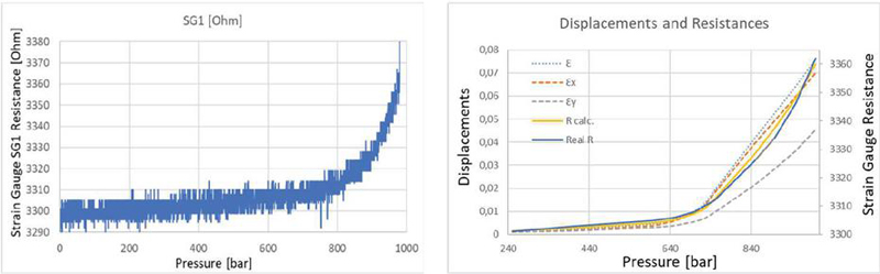
Figure 39 Sensor signal in respect to burst test bench pressure (left), FEM displacement (right).
In fact, the strain gauge changes its resistance based on a gauge factor G that is the sensitivity of the strain gauge and it represents the ratio between the resistance variation and length variation of the strain gauge. The G factor of the strain gauge it results 0,4, a limited value in respect to commercial strain gauges, but it is due both to its length characteristics and the fact that not all the strain gauge is involved in the pole tube deformation.
Table 5 FEM and real data for pressure test: 2-SG Sensor
| Pressure [bar] | R [ohm] | R [ohm] | Var % | |||
| 250 | 0,00128 | 0,001 | 0,00101 | 3301,3332 | 3301 | 0,04% |
| 400 | 0,00231 | 0,00187 | 0,0017 | 3302,244 | 3303 | 0,07% |
| 600 | 0,00463 | 0,00395 | 0,00313 | 3304,1316 | 3305 | 0,13% |
| 650 | 0,00647 | 0,00575 | 0,0039 | 3305,148 | 3306 | 0,16% |
| 700 | 0,0101 | 0,00926 | 0,00554 | 3307,3128 | 3308 | 0,22% |
| 725 | 0,0131 | 0,0122 | 0,00684 | 3309,0288 | 3310 | 0,27% |
| 750 | 0,0191 | 0,018 | 0,00945 | 3312,474 | 3312 | 0,38% |
| 850 | 0,0418 | 0,0395 | 0,0215 | 3328,38 | 3326 | 0,86% |
| 900 | 0,0527 | 0,0495 | 0,0284 | 3337,488 | 3334 | 1,14% |
| 950 | 0,064 | 0,0596 | 0,0363 | 3347,916 | 3346 | 1,45% |
| 1000 | 0,0758 | 0,07 | 0,0454 | 3359,928 | 3362 | 1,82% |
With the gauge factor G and the resistance in nominal condition R it is possible to calculate the resistance that the strain gauge should have in the different FEM conditions of simulation. R value is the value without strain at the temperature of the test. In this case R is the value acquired by the test bench in 1 bar pressure condition.
| (10) |
The Equation (10) is the law for calculating the strain gauge resistance. In the equation G 0,4 and R ohm, is the strain, the measure of change in length due to pressure. In the case of the strain gauge wrapped in the pole tube, the strain in the circumferential direction is chosen, due to the orientation of the conductive tracks of the strain gauge used that are in the circumferential direction of the pole tube. These calculated values can be compared with the real data acquired at test bench shown in the left graph of Figure 39, sampling the data from the test bench at the pressure values of interest, the same of FEM simulations pressure values. In Table 5 the strain , the strain in radial direction and the strain in circumferential direction calculated by the FEM simulations are reported at different pressure values. In the last two columns of the Table there are R, the resistance of the strain gauge calculated using the of the FEM and Equation (10), the R, obtained from experimental data at the burst test bench (Figure 39 left graph) and the percentage variation with respect the nominal resistance.
The same data are shown in the right graph of Figure 39. In the graph, the dotted lines are (equivalent, it’s an average of the two in x and y coordinates), and , while the continuous lines are R and R, respectively in yellow and blue colors. It can be seen that the two lines of R and R in the graph have a good correlation and that there is correspondence between the FEM data and the experimental data. This test validates the strain gauge data acquired in the burst tests.
Table 6 FEM and real data for pressure test: 4-SG sensor
| Pressure [bar] | R [ohm] | Var % | |||
| 250 | 0,00128 | 0,001 | 0,00101 | 900,909 | 0,10% |
| 400 | 0,00231 | 0,00187 | 0,0017 | 901,53 | 0,17% |
| 600 | 0,00463 | 0,00395 | 0,00313 | 902,817 | 0,31% |
| 650 | 0,00647 | 0,00575 | 0,0039 | 903,51 | 0,39% |
| 700 | 0,0101 | 0,00926 | 0,00554 | 904,986 | 0,55% |
| 725 | 0,0131 | 0,0122 | 0,00684 | 906,156 | 0,68% |
| 750 | 0,0191 | 0,018 | 0,00945 | 908,505 | 0,94% |
| 850 | 0,0418 | 0,0395 | 0,0215 | 919,35 | 2,15% |
| 900 | 0,0527 | 0,0495 | 0,0284 | 925,56 | 2,84% |
| 950 | 0,064 | 0,0596 | 0,0363 | 932,67 | 3,63% |
| 1000 | 0,0758 | 0,07 | 0,0454 | 940,86 | 4,54% |
With the new sensor version, where 4 SGs of different shape and dimensions are placed along the entire pole tube, the central ones (SG2 and SG3) cover the region around the control cone subjected to fatigue breakage and SG1 is over the hollow part of the pole tube more subject to pressure strain. The same considerations on the sensor sensitivity and gauge factor G made for the 2 SGs sensor can be done for the new sensor, but now the gauge factor G can be evaluated equal to 1, like in the traditional strain gauges, as a consequence of the fact that the entire area of the sensor is now affected by the deformation due to pressure strain or to malfunction resulting from fatigue failures, so that the resistance variation is on its entire length.
The considerations remains the same done before, and we consider the same law to describe the strain gauge resistance, but now G 1 and RR900 ohm. In Table 6 the strain , the strain in radial direction and the strain in circumferential direction calculated by the FEM simulations are reported at different pressure values. In the last two columns of the Table 6 there are R, the resistance of the strain gauge, calculated using the of the FEM and Equation (10), and the percentage variation with respect the nominal resistance.
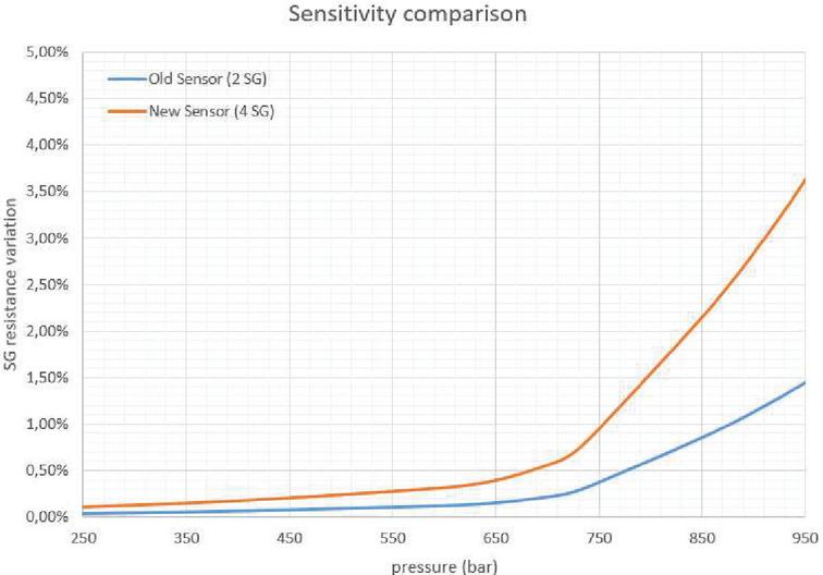
Figure 40 Sensitivity comparison between 2SG sensor and SG2 and SG3 of the 4 SG sensor.
In Figure 40, the comparison between the percentage changes in sensor resistance value with respect to pressure are shown. The graph demonstrates the possibility to increase the sensor sensitivity applying a sensor design with the constraint that the deformation affects the entire area covered by the sensor, thus realizing a sensor capable of an earlier abnormal condition detection. The described experience only covers one of the type of failure of the valve due to pressure. Endurance tests, executed to calculate the MTTF (Mean Time To Failure) and MTTFd (MTTF dangerous), and to evaluate if the sensor is capable to measure the residual life instead allowed to discover other types of faults, which are more difficult for the sensors to detect and measure.
Company’s previous experiences on valve testing have shown that valves can break in two main ways: due to excessive pressure, as described in the previous chapter, and due to fatigue. The fatigue failure is more challenging in terms of its diagnosis and predictive diagnosis, because the failure occurs in the absence of particular deformation due to yielding of the metals. A test campaign with endless sessions of continuous pressure transients was carried out, in order to reproduce an accelerated aging of the component and reproduce the conditions for fatigue failures. Due to quality of component a higher pressure have been used to accelerate the ageing process, using 430 bar instead of the maximum nominal pressure of 250 bar.
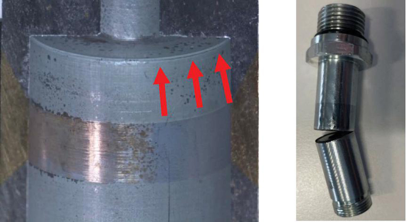
Figure 41 Creak of the pole tube near control cone (left) and valve broken (right).
Fatigue failure occurs mainly due to the notch effect in the section restriction near the control cone. The limited radius at the bottom of the drilled hole (shown by red arrows in Figure 41) presents a stress peak that brings to breakage with repeated loading fatigue (from P to P).
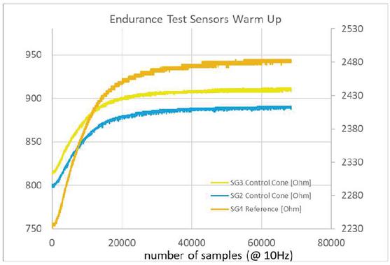
Figure 42 Thermal strain during test bench warm up.
Endurance tests have shown a progressive weakening of the area and the appearance of cracks near the control cone (Figure 41), with consequent oil vaporization and subsequently with oil spillage and finally with significant oil leaks, which can cause dangerous failures, depending on the application in which the cartridge valve is used. As it can be seen from the warming up diagrams from Figure 42, the fatigue test bench was started each morning to allow real-time monitoring throughout test session and the strain gauges had a warm up period, during which all the resistances changed due to changes in oil temperature. After this warm up period, the resistances presented always constant values: the reference one under 2500 ohm (around 2480 ohm), while the two smaller faced to the two welded-brazed interfaces of the control cone around 890 and 910 ohm respectively. In fact, all sensors are affected by the thermal strain and it must be considered because it is not a dangerous strain to be diagnosed, but it is a normal strain that needs to be recognized. The parameter which allows to evaluate it properly is whether all strain gauges of the sensor increase strains with an equivalent percent, as is in Figure 42.
In the figure, both SG2 and SG3, the two sensors facing the welded-breezed surfaces of the control cone change their resistance due to thermal expansion with the same shape and so is for SG4, the reference resistance facing the solid part of the pole tube of the valve.
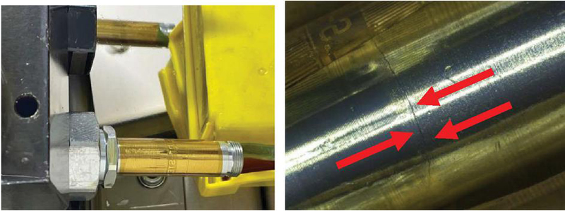
Figure 43 Valve with four strain gauges sensor during endurance test.
The Valve under test (Figure 43, left) has been analysed after the fault and it has been found the classic crack near the control cone as shown in Figure 43, right side, where the sensor completely broken by the oil pressure is shown and where the crack is highlighted by the red arrows. Indeed, one of the choice made for the prototypes was to glue only the axial-ending locations of the sensor, so if oil is spilling from the pole tube, all strain gauges are affected by the change in volume. This choice was made for the easiness of gluing the external perimeter instead of the entire surface of the sensor. Therefore, in the next tests all strain gauges will change their strain when valve breaks. If glue was on the entire surface of the sensor, it was likely that the strain changed only for the strain gauge faced with the crack, or in the event that the strain gauge was broken by the oil spilling under pressure, making easier to recognize a valve fault.
The case described, is the one under analysis and it shown in Figure 44. In this test, when the pole tube started to present the first crack, the strain gauges resistance suddenly overcome the normal values, remaining for long time in an abnormal resistance condition during which the valve was running properly, but with some oil vaporization under the skin of the sensor. This condition is stable until the crack opens.
The time period from the first invisible crack with oil vaporization and the presence of a dangerous crack in the pole tube can vary, but is always more than 10 minutes in the high stress condition of the endurance test, where transients from 0 to 430 bar were continuously repeated at 3 Hz (3 transient for each second).
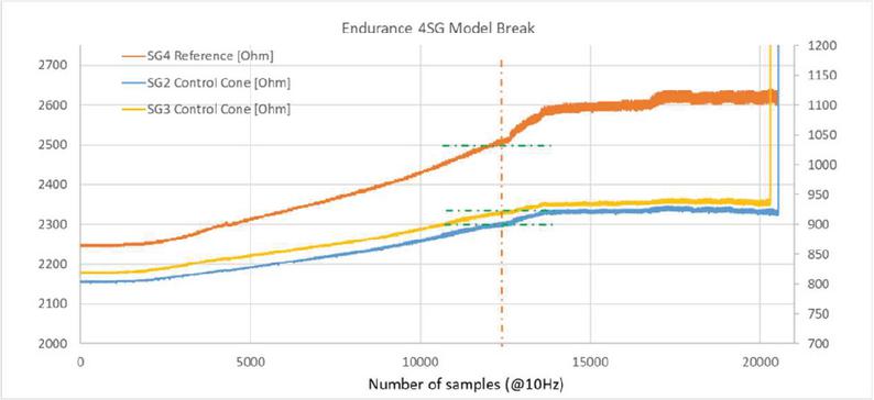
Figure 44 Four strain gauges sensor breakage during endurance test.
In the Figure 44, for example, the time period from 12.500 samples to 20.500 samples is the period during which the sensors present abnormal values, but the valve continues to operate without any visible malfunction. This period is approximately 8.000 test bench samples at 100 ms of time period, corresponding to more than 13 minutes. This test demonstrates that the new sensor is capable of detecting, recognizing and signalling an abnormal valve condition, due to the fatigue fracture of the valve’s pole tube, despite the absence of a pole tube deformation. This is due to the pressure to which the strain gauges are subjected, due to the vaporization of oil at high pressure in the volume created between the sensor and the valve pole tube.
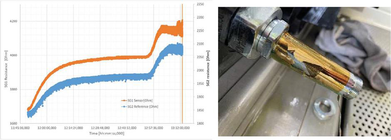
Figure 45 Two strain gauges sensor breakage during endurance test.
Similar tests were carried out also testing the first version of the sensor, made up of two strain gauges, the first facing the hollow area of the pole tube, that corresponds to the volume where it is working the moving armature, the second facing the solid part of the pole tube, used as a reference, because it is subject to only temperature strain.
As it was presented in [23], the pressure tests carried out on this two strain gauges model showed that it was very easy to diagnose, due to the change in shape of the pole tube under excessive pressure or due to some material enervation. This incoming fault condition allowed the acquisition of a difference between the changes in resistance of the two sensors, quite different from the one due to temperature strain.
In that case, both strain gauges changed their resistance due to oil vaporization and, in subsequent time, due to oil spilling, which created a change in shape of the whole sensor due to the chosen gluing method. But, even in this case, the resistance of both strain gauges reached values not in line with the temperature and, after more than 16 minutes (around 3.000 cycles of the pressure transient from tank pressure – near 1 bar – to 430 bar), one of the sensor was broken by the oil pressure spilling in the volume between the sensor and the valve. The results of this test are presented in Figure 45, where in the left diagram is visible the transient and the final breakage of the SG1 sensor, and in the right the result of the breakage due to the oil spilling under pressure. Also in the case of the two strain gauges sensor, the sensor was found able to diagnose an abnormal condition indicating impending valve failure due to fatigue stress.
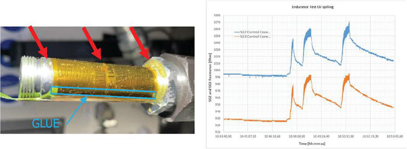
Figure 46 Sensor functionality with oil loss, gluing area is highlighted in the figure.
Finally, it was tested what happens in cases where the oil is spilling and it breaks the glue resulting in an oil loss without a sensor breakage. In one of the endurance tests a sensor glued only along the pole tube and not along the circumference was used, to allow the oil spilling. At the end of the test the oil spilling was observed, but also an abnormal strain, with the difference that the strain was repeated for each test bench cycle, without breaking the sensor. The result is shown in Figure 46. As it can be noted, the pressure is sufficient to induct an abnormal strain and then to allow the pole tube fault diagnosis.
The test was conduct stopping the continuous cycling at 3 Hz of 430 bar pressure peak transient, and some slower test at 250 bar was executed, in order to understand if at nominal pressure the fault could be recognized. As it is shown in the figure, the strain gauges resistance change from 995 to 1070 for SG2 and from 930 to 990 for SG3 with a percent change of 5,8 % and 7,5% respectively (due to the relative position of the breaking crack). Both the absolute value of resistance transient, the dynamic of the transient and the different in percent values allow to immediately diagnose an abnormal condition for the valve. In fact the normal thermal expansion, the only one that the sensor is able to acquire in normal operating conditions, could not have presented either the dynamic one, nor those absolute values and above all it could not have presented different variations for the two sensors at the two ends of the control cone.
To collect a more comprehensive set of tests, another test was performed. Two valves have been tested together, one with coil mounted and one without. The coil changes the shape of the sensor once the oil start vaporization or spilling due to a crack, the reference sensor is less affected by the change of shape and change in resistance. The test with breakage of the valve with coil is shown in the Figure 47.
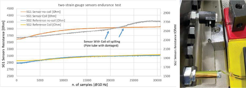
Figure 47 Two-SG valve with and without coil under test, valve damaged.
In the figure there are two aspects to be noted: the first one, is that the valve with coil shows a different warm-up curve both in the yellow line, SG2 reference, and gray line, SG1 sensor, in respect to the valve without coil; the second aspect is that, when the pole tube is damaged, the sensor SG1 (grey line) starts changing its shape and changes its resistance accordingly, while the reference SG2 doesn’t change its resistance, because the oil doesn’t reach the pole tube area of the reference strain gauge.
In the latter case the diagnosis is easier and does not need any other sensor (like an oil temperature sensor) to immediately recognize an abnormal condition that is probably related to a fatigue failure. As previously underlined, also in this case from the time when the sensors recognize the abnormal condition, to the time when the sensor breaks or the oil start spilling a dangerous amount of oil, there are more than 13 minutes. In fact in the figure the change of resistance starts from around 22.500 number of cycles to more than 30.000 number of cycles before the sensor SG1 breaks, at 10 cycles per second.
This test concludes the experimental part of the research work and allows to state that the new hyper-thin sensors are able to diagnose the pole tube faults of cartridge valves under all possible conditions.
This project represents the first complete experience of implementation of new hyper-thin sensors to cartridge valves; the use cases and the tests executed cover the most likely real conditions, especially those related to endurance tests. The sensors presented are specialized versions of multiple strain gauge sensors. These sensors are not only special in their shape, but both materials and process are new for this application field. A very thin substrate and a nano-metric conductive material deposition, as well as the design freedom offered by the flexible electronics, have made it possible to generate a series of sensors capable of detecting phenomena that normal strain gauges were unable to detect in past experiences. Besides it has been demonstrated that it is possible to create custom hyper-thin strain gauges of around 10 m of thickness with useful resistance values for application in cartridge valves and, in general, in hydraulic components.
The lesson learned includes the awareness that a specialized sensor design increase the sensitivity and the usefulness of the sensor itself. To design the perfect sensor and to include it in a modified component without losing performance, many expertise are required, from materials, processes knowledge to mechanical and simulation design to electromagnetic analysis, until analogue and digital electronic hardware and software design.
The new sensor, in all the versions presented, is a safety relevant sensor for cartridge valves, which allows detecting abnormal pole tube deformation at early stage, before experiencing a valve breakage or oil leaks due to valve cracks. The new sensor represents a major step in valve diagnostics and prognostics, because it allows direct measurement of the pole tube strain, preventing breakage and oil leaks, which were previously detectable indirectly by pressure sensors in the manifold or in the hydraulic pipes, but only when the pressure in the circuit drops due to a macroscopic oil leak. Early identification of preventative diagnostic conditions is essential to making valve-based systems safer.
The sensors demonstrated their efficacy in both static and dynamic conditions, in pressure (burst) and endurance tests, both with and without coil, and have been characterized until sensor breakages and valve breakages through real test campaigns. The sensors are able to detect and diagnose all faults, with some difference in the “fault distance” but always at early stage.
This research demonstrates that shape design freedom offered by flexible electronics technology represents an interesting opportunity to equip hydraulic components with new sensors, which can bring to electro-hydraulic systems an unseen diagnostic coverage level.
This sensor matches with the most stringent requirements of diagnostic coverage of fault tolerant applications and it is able to prevent dangerous faults with a significant time advance, helping manufacturers to make safer and reliable hydraulic systems. These sensors could represent an important advancement for the design of electro-hydraulic systems in various challenging fields and applications, such as: naval and submarine, avionics, autonomous, robotics or assisted systems, steering and braking, and in military applications.
The research was carried out under the financed project “Mechatronic hydraulic valves equipped with innovative intrinsically safe sensors” granted to VIS Hydraulics Company under the Italian Law 14/2014 for European funding for regional development.
[1] Jingqi Liu, Chenggang Yuan, Lukas Matias, Chris Bowen, Vimal Dhokia, Min Pan, James Roscow, Sensor Technologies for Hydraulic Valve and System Performance Monitoring, Challenges and Perspectives. Advanced Sensor Research. 2024. doi: 10.1002/adsr.202300130.
[2] A.I. Pavlov, I.A. Polyanin, K.E. Kozlov, Improving the Reliability of Hydraulic Drives Components, Procedia Engineering, Volume 206, 2017, Pages 1629–1635, ISSN 1877–7058, https://doi.org/10.1016/j.proeng.2017.10.689.
[3] B. Beck, J. Weber, Enhancing safety of independent metering systems for mobile machines by means of fault detection, The 15th Scandinavian International Conference on Fluid Power, SICFP’17, June 7–9, 2017, Linköping, Sweden, ISBN: 978-91-7685-369-6, ISSN: 1650-3686 (tryckt), 1650-3740 (online), http://dx.doi.org/10.3384/ecp1714492.
[4] Jinchuan Shi, Jiyan Yi, Yan Ren, Yong Li, Qi Zhong, Hesheng Tang, Leiqing Chen, Fault diagnosis in a hydraulic directional valve using a two-stage multi-sensor information fusion, Measurement, Volume 179, 2021, 109460, ISSN 0263-2241, https://doi.org/10.1016/j.measurement.2021.109460.
[5] Nurmi, J, & Mattila, J. “Detection and Isolation of Faults in Mobile Hydraulic Valves Based on a Reduced-Order Model and Adaptive Thresholds.” Proceedings of the ASME/BATH 2013 Symposium on Fluid Power and Motion Control. Sarasota, Florida, USA. October 6–9, 2013. V001T01A020. ASME. https://doi.org/10.1115/FPMC2013-4435.
[6] L. Siivonen, M. Huova, and M. Vilenius. Fault Detection and Diagnosis of Digital Hydraulic Valve System. The Tenth Scandinavian International Conference on Fluid Power, May 21–23, 2007 Tampere, Finland, Tampere, 2007.
[7] J Ersfolk, M Ahopelto, W Lund, J Wiik, M Waldén, M Linjama, J Westerholm, Online fault identification of digital hydraulic valves using a combined model-based and data-driven approach, arXiv preprint arXiv:1803.05644, 2018arxiv.org, https://doi.org/10.48550/arXiv.1803.05644.
[8] Denkena, Berend & Dahlmann, Dominik & Kiesner, Johann. (2014). Sensor Integration for a Hydraulic Clamping System. Procedia Technology. 15. 10.1016/j.protcy.2014.09.006. https://doi.org/10.1016/j.protcy.2014.09.006.
[9] Guo, Yuan, Zeng, Yinchuan, Fu, Liandong and Chen, Xinyuan. (2019). Modeling and Experimental Study for Online Measurement of Hydraulic Cylinder Micro Leakage Based on Convolutional Neural Network. Sensors. 19. 2159. 10.3390/s19092159.
[10] Liu, J., Yuan, C., Matias, L., Bowen, C., Dhokia, V., Pan, M. and Roscow, J. (2024), Sensor Technologies for Hydraulic Valve and System Performance Monitoring: Challenges and Perspectives. Adv. Sensor Res., 3: 2300130. https://doi.org/10.1002/adsr.202300130.
[11] Fu-qiang Chen, Ming Zhang, Jin-yuan Qian, Yang Fei, Li-long Chen, Zhi-jiang Jin, Thermo-mechanical stress and fatigue damage analysis on multi-stage high pressure reducing valve, Annals of Nuclear Energy, Volume 110, 2017, Pages 753–767, ISSN 0306-4549, https://doi.org/10.1016/j.anucene.2017.07.021.
[12] Georgy M. Makaryants, Fatigue failure mechanisms of a pressure relief valve, Journal of Loss Prevention in the Process Industries, Volume 48, 2017, Pages 1–13, ISSN 0950-4230, https://doi.org/10.1016/j.jlp.2017.03.025.
[13] R.T. Byrnes, S.P. Lynch, An unusual failure of a nickel-aluminium bronze (NAB) hydraulic valve, Engineering Failure Analysis, Volume 49, 2015, Pages 122–136, ISSN 1350-6307, https://doi.org/10.1016/j.engfailanal.2014.11.009.
[14] Jilai Cao, Jian Zhang, Xinhai Yu, Shan-Tung Tu, Detection of pressure relief valve leakage by tuning generated sound characteristics, Process Safety and Environmental Protection, 148, 2021, Pages 664–675, ISSN 0957-5820, https://doi.org/10.1016/j.psep.2021.01.050.
[15] A.K. Bose et al., “Screen-Printed Strain Gauge for Micro-Strain Detection Applications,” in IEEE Sensors Journal, vol. 20, no. 21, pp. 12652–12660, 1 Nov.1, 2020.
[16] Araromi, O.A., Graule, M.A., Dorsey, K.L. et al. Ultra-sensitive and resilient compliant strain gauges for soft machines. Nature 587, 219–224 (2020).
[17] A. K. Bose et al., “Screen-Printed Strain Gauge for Micro-Strain Detection Applications,” in IEEE Sensors Journal, vol. 20, no. 21, pp. 12652–12660, 1 Nov.1, 2020, doi: 10.1109/JSEN.2020.3002388.
[18] F. Maita, V. Piccialli, F. Pensa, M. Scatto, M. Ruggeri and L. Maiolo, “Application of Unconditioned Nanostructured Thermoplastic-Based Strain Gauge Sensor in Wearable Electronics,” in IEEE Sensors Journal, vol. 22, no. 24, pp. 24019–24026, 15 Dec.15, 2022.
[19] Irani, F.S.; Shafaghi, A.H.; Tasdelen, M.C.; Delipinar, T.; Kaya, C.E.; Yapici, G.G.; Yapici, M.K. Graphene as a Piezoresistive Material in Strain Sensing Applications. Micromachines 2022, 13, 119.
[20] A. Pecora et al., “Strain gauge sensors based on thermoplastic nanocomposite for monitoring inflatable structures,” 2014 IEEE Metrology for Aerospace (MetroAeroSpace), Benevento, Italy, 2014, pp. 84–88.
[21] Li, H., Zhang, J., Chen, J. et al. A Supersensitive, Multidimensional Flexible Strain Gauge Sensor Based on Ag/PDMS for Human Activities Monitoring. Sci Rep 10, 4639 (2020).
[22] E Aslanidis, E. Skotadis and D. Tsoukalas, Resistive crack-based nanoparticle strain sensors with extreme sensitivity and adjustable gauge factor, made on flexible substrates, Nanoscale, 2021, 13, 3263–3274.
[23] Massimiliano Ruggeri, Francesco Maita, Luca Maiolo, Mattia Ferri, Christopher Rosi and Sara Baldoni Innovative hyper-thin sensor for cartridge valves diagnostics and prognostics, Proceedings of MAHA 2024 Fluid Power Conference, 1–3 Sept. 2024 Purdue University, Lafayette, Indiana, e-ISBN: 9788770047456, doi: 10.13052/rp-9788770047456.009.
[24] M. Ruggeri, F. Maita, L. Maiolo, M. Braiato, C. Gialluca, D. Guidi, Novel Hyper-Thin Strain Gauge Sensors for Cartridge Valves, JFPS 2024, Japan Fluid Power Symposium 2024, Hiroshima October 22–25, 2024.
[25] Y.-n. Wang et al., “Characteristics and electrical properties of polyimide films fluorinated for different durations”, Materials Today Communications 26 (2021) 102098, https://doi.org/10.1016/j.mtcomm.2021.102098.
[26] N Khomiakova et al., Investigation of Wettability, Drying and Water Condensation on Polyimide (Kapton) Films Treated by Atmospheric Pressure Air Dielectric Barrier Discharge, Coatings 2020, 10(7), 619, https://doi.org/10.3390/coatings10070619.
[27] W. Chen et al., “Customized surface adhesive and wettability properties of conformal electronic devices”, Mater. Horiz., 2024, 11, 6289–6325 https://doi.org/10.1039/D4MH00753K.

Massimiliano Ruggeri received the master’s degree in electronic engineering from Bologna University in 1995, and the Ph.D. degree in Management Engineering from Modena and Reggio Emilia University in 2009. He is currently working as a researcher at the Institute for Energy and Sustainable Mobility – STEMS, of CNR, the National Research Council of Italy. He is also Government Expert for Land Technologies for the Italian Ministry of Defence at European Defence Agency. His research areas include mobile mechatronics and hydraulics, sensors and actuators, mobile robotics, functional safety systems, as well as embedded systems and controls.

Francesco Maita received the M.Sc. (cum laude) degree in Electronics Engineering and the Ph.D. in “Engineering of Sensorial and Learning Systems” both from the “Università degli studi di Roma Tor Vergata”, in 2008 and 2013, respectively. He worked as a post-doctoral researcher at the Institute for Microelectronics and Microsystems of the CNR of Rome from 2012 to 2016. Since 2017, he works as a researcher at the same institution. His research activity focuses on electronic design, fabrication and characterization of smart circuits for sensing, with a specific focus on flexible devices.

Luca Maiolo received the Master degree in Physics in 2003 and the Ph.D. in 2008, both from “Università degli studi di RomaTre”. Currently, he works as senior researcher at the Institute for Microelectronics and Microsystems of the National Research Council (CNR-IMM). His work primarily focuses on the fabrication and characterization of ultrathin flexible sensors for biomedical, automotive, and aerospace applications. He has authored over 150 peer-reviewed papers in international journals and serves as a rapporteur for the Italian Ministry of Economic Development in the field of nanotechnologies.

Ivano Lucarini is a physicist with a M.Sc. in condensed matter physics and a Ph.D. in applied electronics, both obtained from “Roma Tre University”. He pursued his doctoral research in collaboration with the Institute of Microelectronics and Microsystems (IMM) of the Italian National Research Council (CNR). Currently, he serves as a technologist at the CNR-IMM’s Rome location, specializing in the microfabrication of electronic, electrical, and microelectromechanical devices, including flexible designs. His expertise covers thin film deposition and patterning, utilizing optical photolithography techniques.

Mattia Ferri received the M.Sc. in Electronics Engineering from the University of Ferrara in 2015. He started his career in E.S.T.E. S.r.l. Company as hardware and firmware designer. He is now head of hardware design department of the company. He has been part of 2 EU ECSEL projects and principal investigator of an EIT Manufacturing project, as well as of some national and regional financed projects.

Christopher Rosi received the Master’s Degree on Electronics Engineering from the “Enzo Ferrari” Department of Engineering of the University of Modena and Reggio Emilia in 2020. He started his career at VIS Hydraulics in 2020 as a member of the Research and Development Department of VIS Innovation centre and his activities include projects related to sensorization and electronic control of cartridge valves, FEM electromagnetic simulations, lumped parameter simulations and data analysis.

Chiara Gialluca received the Master Degree on Materials Engineer from “Enzo Ferrari” Department of Engineering of the University of Modena and Reggio Emilia in 2017. She started her career in a polymer Company, after which she continued her career at VIS Hydraulics in March 2023 as member of the Research and Development of VIS Innovation centre and her activities include project related to thermal and surface treatments of metallic materials, research, testing and validation of new high-performance materials for cartridge valves, structural FEM simulation and data analysis.

Sara Baldoni received the Master’s Degree on Mechanical Engineering from the “Enzo Ferrari” Department of Engineering of the University of Modena and Reggio Emilia in 2008. She started her career at VIS Hydraulics in April 2009 as Mechanical Designer and, after having gained a wide experience in the engineering field, she’s now in charge of the Research and Development Department at the VIS Hydraulics Innovation Centre.
International Journal of Fluid Power, Vol. 26_2, 211–262.
doi: 10.13052/ijfp1439-9776.2625
© 2025 River Publishers