On the Volumetric Loss Caused by Incomplete Filling with Undissolved Gas in Positive Displacement Pumps: Lumped Parameter Modeling, CFD Comparisons, and Experimental Validations
Dinghao Pan1,*, Andrea Vacca1, Venkata Harish Babu Manne2 and Daniel Gysling3
1Maha Fluid Power Research Center, Purdue University, IN, USA
2Simerics Inc, MI, USA
3CorVera LLC, CT, USA
E-mail: pandinghao1@gmail.com; avacca@purdue.edu; mvharishbabu@gmail.com; dgysling@corvera.io
*Corresponding Author
Received 01 January 2025; Accepted 28 February 2025
The analysis of the incomplete filling behavior of positive displacement machines requires considerations of the air content within the fluid and its dependency with the suction conditions, which are often associated with high uncertainties. This study contributes to this topic by experimentally studying the incomplete filling behavior of a positive displacement pump and presenting a hybrid modeling method for predicting it. The experimental study involved an original pump testing setup able to measure the gas volume fraction by interpreting the sound wave transmission behavior. Experimental results show that under same sub-atmospheric pump inlet pressure, low-speed operation can enhance the incomplete filling. This behavior is found related to the transient air release process in the line connecting the upstream pressure restriction location (which regulates the sub-atmosphere line pressure) to the pump, which is an effect often neglected in similar analyses on positive displacement machines that neglects the effect of the suction line. Based on the experimental study, a hybrid modeling method for predicting the volumetric losses caused by incomplete filling is proposed, where (i) the amount of undissolved gas in the hydraulic circuit upstream the pump is evaluated by a 1st-order gas release formulation, and (ii) the pump volumetric loss due to incomplete filling is simulated with a lumped volume-based pump model (LP pump model) with an gas-equilibrium fluid model with an equivalent total gas determined from step (i). The 1st-order gas release prediction approach was validated by CFD results of sub-atmospheric pipe flows, for a range of gas-release 1st-order time constants. Using a time constant of 8 s and total air of 6 %, the 1st-order formulation was also validated with experiments. The volumetric loss predicted by the LP pump model were found to agree with the measured pump volumetric efficiency at different operating conditions. The proposed hybrid approach presents a useful simulation tool for studying the incomplete filling of positive displacement pumps with sub-atmospheric inlet pressures, with consideration concerning the layout of the suction circuit.
Keywords: Incomplete filling of positive displacement pump, undissolved gas measurement, lumped parameter pump model, 1st-order air-release cavitation, equivalent total air, CFD study of pipe transient air releasee.
Incomplete filling in a positive displacement pump means a situation where the displacement chambers of the pump can no longer be filled with the working fluid in the liquid state. When incomplete filling occurs, there is a significant portion of gas filling the displacement chambers, which is caused by the working fluid reaching a pressure lower than the saturation pressure (aeration) or, in extreme cases, vapor pressure (vapor cavitation). This phenomenon is associated with volumetric losses (or incomplete filling losses), as these gases eventually are dissolved back in the fluid at the high-pressure delivery conditions. Besides being an energy loss, incomplete filling should also be avoided because it is often associated with detrimental effects such as noise generation or mechanical damages caused by bubble collapsing.
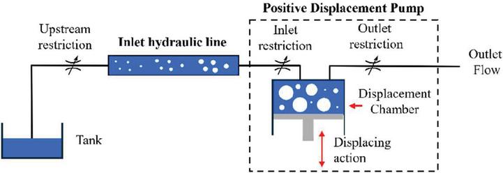
Figure 1 Hydraulic circuit of a pd pump under induced incomplete filling.
As Figure 1 illustrates, incomplete filling often occurs under an excessive pressure loss in a) the line connecting the reservoir to the pump inlet (equivalently caused by an upstream flow restriction) or b) between the pump inlet and its displacement chambers (caused both by the pump inlet restriction and the displacement chamber volume expansion related with the displacing action). Therefore, the phenomenon of incomplete filling is related to both the design of the suction circuit and the pump geometry. Certain pump designs (e.g. internal gear pumps and Ge-rotors) are known for having better filling capabilities due to their lower internal pressure loss [2, 3], although they are still subject to incomplete filling under unfavourably high speeds or if an upstream restriction is present. Note that incomplete filling is related to the high operating speeds not only because of a higher pipe loss, but also because of a more rapid volume expansion of the displacement chambers, which gives higher pressure losses in both types a) and b). Additionally, fluid properties, namely the dissolved air content at the reservoir, where saturation conditions can usually be assumed, also heavily affect the incomplete filling because of aeration. According to Henry-Dalton’s law – in equilibrium conditions the fraction of air released is proportional to the absolute liquid pressure – oil that dissolves more air at atmospheric pressure releases more air after the same pressure drop. Incomplete filling may also be caused by entrapped air (pseudo-cavitation), which is not associated with air release but rather with the air leakage into the suction circuit or tank design limitations [4]. Furthermore, an incomplete filling may rise if the reservoir pressure is below the atmosphere, which is an important aspect for designing aviation hydraulic reservoirs [5]. However, this work will neglect pseudo-cavitation phenomena and a sub-atmosphere tank and focus only on incomplete filling caused by the two types of pressure drops a) and b) mentioned above.
Past researchers have studied the pump incomplete filling behavior using experiments and different modeling techniques involving CFD and Lumped Parameter (LP) based models. Both simulation techniques are closely related to an important fluid property parameter known as the total air. In this paper, the total air is defined by the volume ratio between the total gas content and the total mixture volume after all dissolved and undissolved gas was separated from the liquid and stored at the reference state, as Equation (1) states. Note that such a definition is also often considered in engineering modeling utilities, such as Simcenter AMESim [6].
| (1) |
When simulating incomplete fillings, CFD simulations consider the gas presence with two approaches: equilibrium-CFD (where the undissolved gas fraction is determined from the pressure) and dynamic-CFD (which involves additional transport equations for gas or vapor content). Based on equilibrium-CFD, Altare and Rundo [7] showed that, with an unchanged sub-atmospheric pump inlet pressure, higher speeds lead to more severe incomplete filling in a Gerotor. Such speed dependency was also observed in other equilibrium-CFD-based studies, e.g., Hussain et al. for a Gerotor [8], Corvaglia et al. for an external gear pump [9]. Note this speed dependency was reported as negligible by Fresia et al. [10] for an internal gear pump running a high-viscosity fluid. Altare and Rundo noticed a total air setting of 2% in the simulation matched best with closed circuit experiments, indicating that the total air (which is commonly found for open reservoirs [11]) should not be generalized to various circuits. Fresia et al. [10] explained the better matching from the low air content as, before the pump inlet, the pump was only drawing the oil but without separating the air. Furthermore, based on equilibrium-CFD, Pleskun et al. [12] predicted the incomplete filling behavior for a screw pump, Boland and Shang [13] studied the scalability for the incomplete filling phenomenon, and Rundo et al. [14] investigated the impact of inlet geometries of a vane pump’s filling capability under atmosphere inlet pressure. With the dynamic-CFD approach, on the other hand, Buono et al. [15] studied the incomplete filling of a Gerotor, reporting 8% total air simulation matching the measured flow saturation. Similar studies can be found by Stuppioni et al. [16] for a vane pump and by Yin et al. [17] for a piston pump. Popular dynamic-CFD models, such as the full cavitation model introduced by Singhal et al. [18], often require empirical time constants to describe the speed of phase change processes, including vaporization/condensation and aeration/dissolution. Early experiments from Schweitzer and Szebehely [11] reported s half release time for dissolved air in hydraulic oils. Measurements from Kowalski et al. [19] showed that air release is much slower than vaporization if water is below vaporization pressure, and Yang et al. [20] reported that dissolution is further slower than the air release for the same pressure differential. Notable simulation-based work from Stuppioni et al. [16, 21] investigated how the outlet flow and pressure ripple of a pump with atmospheric inlet pressure could change under different time constant settings in the dynamic-CFD framework, reporting air release time and dissolution time matched best with measurements, and concluding these time constants as critical for describing the gas dynamics in the simulations. More details on different dynamic-CFD models can be found in the review paper from Orlandi et al. [22].
In studies that investigated the incomplete filling behavior with the LP simulation approach, there is also the static cavitation model (where the fractions of vapor and released gas are pressure-dependent) and the dynamic cavitation approach (where the vapor and released gas fraction are solved from the rate equations). Casoli et al. [1] formulated a static model to consider the fluid property change under sub-atmosphere conditions and noticed both a higher total air content and a higher saturation pressure emphasized the incomplete filling prediction. Vacca et al. [23] used a similar implementation to study the incomplete filling behavior of an axial piston pump, discussing the necessity of tuning the model parameters to achieve a higher fidelity compared to experiments. On the other hand, dynamic cavitation models have recently been explored for LP simulations, as can be found in the work from Zhou et al. [24], Shah et al. [25], and Mistry and Vacca [26], involving similar time constants discussed for dynamic-CFD as well. The work from Rundo et al. [27] detailed these time constants based on pump flow and pressure ripples and suggested release time and dissolution time for pumps with atmospheric inlet pressure. However, relevant studies on the incomplete filling behavior have not yet been presented from LP simulations based on dynamic cavitation considerations.
Previous studies on pump incomplete filling often focused on the pump side and didn’t quantify the impact of the two types of pressure drops illustrated in Figure 1. Additionally, although past incomplete filling simulations have widely investigated the fluid settings such as total air and their effects on prediction accuracy, whether the best-matching fluid parameters (total air) can be justified with the design of the circuit has not been understood.
This paper investigates the incomplete filling behavior of a positive displacement pump. In Section 2, the test rig setup developed to consider the two stages of pressure drops illustrated in Figure 1 is presented. With the setup, different operating speeds were measured, including the measurement of the delivery flow, the pressure at the pump inlet, and the gas void fraction (GVF) in the hydraulic line before the pump inlet. Section 3 compares the measured GVF with analytical evaluations derived based on the 1st-order air release assumption. Section 4 presents CFD studies for pipe flows downstream restriction orifices, which demonstrated the effectiveness as well as the limitation of the analytical evaluation. Section 5 presents modeling evaluation of the reference pump’s flow behavior under incomplete filling conditions and compares these results with the experimentally measured flow rates. The whole pump model considered a static cavitation-based method. In the model, the key simulating parameter: total air, was studied and compared with the pump inlet air measurements, from where an alignment was observed between simulations and experiments. Section 6 concludes the major findings of the paper.
The setup for measuring the incomplete filling behavior for a reference 8 cc/rev internal gear pump [28] is illustrated in Figure 2. Valve 1 regulates the pump inlet pressure, and valve 2 is set to fully open to minimize the pressure load on the pump outlet. Such arrangements minimize the effect of pump internal viscous leakage when quantifying the incomplete filling. The test setup also includes an air valve, which was constantly closed during the test. Such a valve allows tests with entrained air, which will be the subject of future work. Pressure sensors P and P measure the pressure change along the hydraulic lines (HL1 and HL2). More details regarding the components used in the measurements are in Table 1.
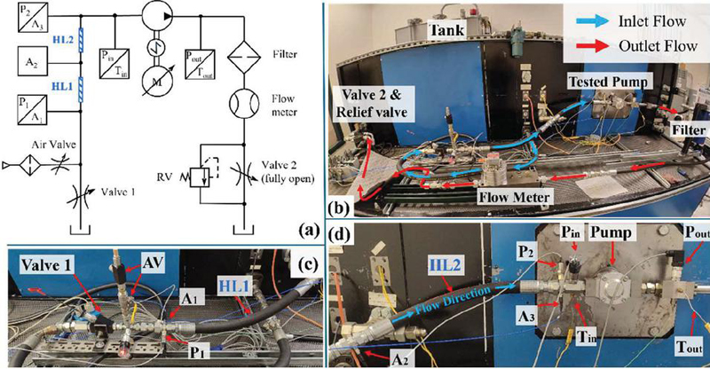
Figure 2 Test circuit to measure the incomplete filling behavior (a: hydraulic circuit; b: overlook of the entire setup; c: inlet region; d: tested pump).
Table 1 Component used in the test circuit
| Components | Parts Used | Accuracy |
| Pump | Eckerle EIPS2-008 | N/A |
| Valve 1 | Sun Hydraulics NFDD-KGN | N/A |
| Flow meter | VSEflow VS 2EPO 12V | 0.3% measured value |
| P | WIKA S-20-1.6 | 0.003 bar |
| P | HAD 4745-B-006-00 | 0.25% measured value |
| A, A, A | PCB 102A44 | 0.07 bar |
| P, P | Keller America absolute type | 0.25% measured value |
| HL1, HL2 | DIN EN 856, inner diameter 1 inch, pipe length 2 feet | |
| Tank | Contains 290-liter hydraulic fluid | |
Notably, this work utilizes a non-intrusive, in-line, real-time, SONAR-based measurement system to quantify the gas void fraction (GVF) in the fluid entering the pump inlet. Based on beam-forming principles, the measurement system calculates the fluid’s speed of sound utilizing the output of three acoustic pressure sensors (A, A, A). The measured sound speed is then interpreted in terms of the gas void fraction utilizing Wood’s equation [29], which provides the direct output of GVF values from the measurement system. For clarity, the GVF measured here is the ratio of the gas volume to the total fluid volume from an imaginary photo of a fluid section inside the circuit where the liquid or the bubbles are not moving. This GVF definition differs from the volumetric ratio between the gaseous and mixture flow rates if the gas and liquid travel at different velocities. For homogeneous conditions assumed in this work, however, where the velocity of the gas phase approaches that of the liquid phase (generally true for low GVF scenarios), the two definitions become equivalent. More details on the measurement approach can be found in Gysling [30].
ISO-VG 46 hydraulic oil under a controlled 23C inlet temperature was used during the test. Four operating speeds (500, 1000, 1500, 2000 rpm) were tested with different pump inlet pressures (measured by P), which were regulated by valve 1. During the test, a loud hissing noise was heard when the pump inlet pressure fell below 0.2 bar absolute, with a spatial location near the outlet port on the pump body. Such pressure limit appeared to be lower for the low-speed conditions: for 500 rpm such limit was 0.18 bar absolute, whereas for 2000 rpm the limit was 0.3 bar absolute. The noise was believed to be related to the fierce vapor bubble collapsing process on the pump outlet side. All measurements discussed in this work are above this low-pressure limit to avoid extended pump operation in the possible damaging conditions.
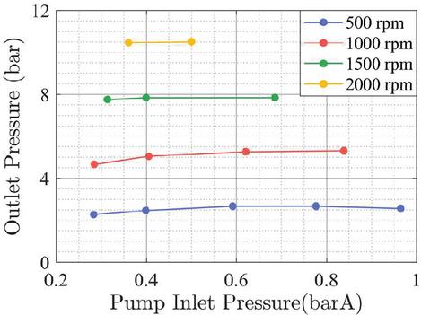
Figure 3 Pump outlet pressure.
It can be noticed from Figure 3 that the upper limit of the tested inlet pressure decreases at higher speeds (from 0.95 bar absolute at 500 rpm to 0.5 bar absolute at 2000 rpm), which is due to the inlet circuit characteristics. Meanwhile, the increase of the pump outlet pressure with the operating speed shown in Figure 3 is caused by the pressure loss characteristics of the outlet circuit. According to the pump specs [28], at 1500 rpm there is a decrease of volumetric efficiency of 0.2% every 8 bar of outlet pressure increase. This justifies that the effect of the measured increase of outlet pressure on the measured volumetric efficiency is minor, and significant volumetric efficiency loss in the measurements should be associated with the incomplete filling phenomenon.
As plotted in Figure 4, the measured pump outlet flow decreases with a lower pump inlet pressure for constant operating speed. Significant flow rate drops happen at pressure values close to the limiting pressure ranges.
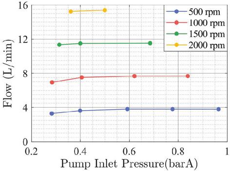
Figure 4 Pump outlet flow.
The impaired outlet flow in Figure 4 represents the incidence of incomplete filling inside the pump, which can be seen more clearly from the volumetric efficiency plotted in Figure 5.
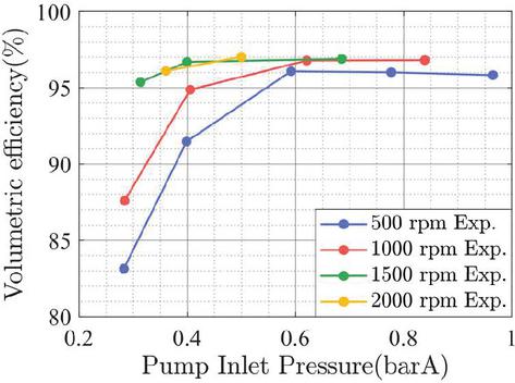
Figure 5 Volumetric efficiency.
Figure 5 shows an interesting trend where, as the speed increases from 500 to 2000 rpm, the incomplete filling becomes less evident for the same inlet pressure. This trend appears to be in contrast with the common belief that higher speeds promote incomplete filling, as reported in several sources [3, 4] and recent works by Rundo [7] and Corvaglia et al. [9]. However, the present paper will show how this trend does not contradict but rather complement the common understanding of incomplete filling. As mentioned in section 1, incomplete filling is caused by the behavior of both the inlet circuit and the pump design. In this test, the effect of the inlet circuit prevails, generating such a trend.
The Gas Void Fraction (GVF) measured are plotted in Figure 6. Note the measurement system calculated the raw GVF around every 2 s, which involves instantaneous oscillations of absolute standard deviation 0.25%. The data reported in Figure 6 averaged a 2-minute period after the on-screen measurement stabilized (which takes about 1 minute). It should be noted that the measured GVFs represent the air volume at sub-atmospheric pressures, not the atmosphere pressure. Also note that the measured GVF can be considered as an averaged measurement at the middle position between hydraulic lines HL1 and HL2, and the gaseous volume entering the pump inlet should be higher than the measured GVF, as the air release process develops along the length of the hydraulic lines. The specific length of the inlet pipes reported in table 1 may be replaced by shorter ones to replicate pump inlet circuits with shorter inlet lines. The capability of current measurement technology in measuring the GVF may be extended for measuring shorter inlet lines. However, that is beyond the current scope and can be a topic of future studies.
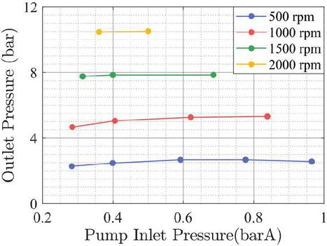
Figure 6 Measured gas void fraction.
The figure shows that as the operating speed increases, the gas volume in the inlet hydraulic lines becomes significantly lower. This trend can be explained as follows: for low speeds, due to the lower mean velocity, the fluid takes a longer time to pass the inlet hydraulic line (see Figure 1), and more air is therefore released into the fluid. Such observed low-speed behavior, despite being related to the inlet circuit design features of (1) considerable circuit length between the restriction and the pump and (2) a variable restriction geometry that allows generating significant pressure drops even at small flowrates, should be carefully considered in practical inlet circuit designs, to prevent the incomplete filling phenomenon for low flow rate conditions.
The GVFs for 1500 and 2000 rpm shown in Figure 6 give a clear clue about the low amount of released air at the pump inlet, which supports the assumption raised by Fresia et al. [10] that under higher flowrates very least air bubbles are released into the fluid before the pump inlet. This assumption well explains why equilibrium-CFD requires a lower total air setting to reproduce the incomplete filling. For 500 rpm operating speed, it takes 10 s for the fluid to pass the total two hydraulic lines, whereas, for 2000 rpm, the travel time becomes 2.4 s. Such difference in the travel time indicates that the time scale of the air release process is on the order of magnitude of seconds, which is consistent with the value found in the measurements by Schweitzer and Szebehely [11]. Note Rundo et al. [27] and Stuppioni et al. [16] reported very fast air release constants () that predicted experiment-matching pump outlet pressure ripples; however, the authors believe the time constants discussed in their work are more related to the fluid-dynamic process inside the pump domain (their work investigated pump with atmospheric inlet pressure), and the process of air release in the circuit upstream the pump inlet should involve a different time constant related to the transient process where the air release process should happen along the flow. Note the latter time constant is expected to be slower than the one discussed in previous researchers’ work, because in the inlet circuit region before the fluid enters the pump, the fluid experience more a calming flowing motion, whereas for the inlet chamber inside the pump housing, e.g., for that of a gear pump, there can be expected continuous and fierce volume expansion process and boundary perturbations due to the gear meshing process.
The air release measured can be compared with the results from an equilibrium fluid model, which states that whenever a pressure change happens to the fluid, the air release and the volume change of the mixture are achieved instantly so that the fluid is always in the equilibrium state. Studies such as [1] and [14] have reported that the fluid equilibrium model when properly tuned, can give a good prediction for the incomplete filling behavior in positive displacement machines. According to the equilibrium fluid model, can be determined according to Henry’s law as Equation (2) gives. Note Equation (2) applies when the fluid pressure is between and and if the fluid pressure is beyond the range, all or none air is released.
| (2) |
The volume of the undissolved air evaluated in Equation (2) must be evaluated at the reference state (, ), as Henry’s law quantifies about the amount of substance rather than the volume. The gas volume expansion caused by pressure decrease can be evaluated with Equation (3). Note the temperature of the left-hand side fluid in Equation (3) is different from the liquid temperature and can be solved from based on the ideal gas law.
| (3) |
The equilibrium fluid model assumes the air release process to happen instantly, whereas in reality, such equilibrium takes time to achieve. In fact, the air release process in hydraulic oils has been reported to have a proportional relationship with the extent of phase imbalance [11]. Based on this idea, a 1storder model is often used to study the transient air release in fluid, of which the applications can be found in Simerics MP+ [16], ANSYS CFX [20], and AMESim [6, 27].
The key idea of the 1st-order air release model can be expressed in the Lagrangian form for a moving fluid element with a specific mass (no mass transfer between surrounding fluid elements), as Equation (4) gives.
| (4) |
In the equation, is the volume of the gas released into the fluid element after time (at no air is released) under pressure . is the equilibrium volume solved from Equation (3). Equation (4) can also be alternatively expressed with mass terms; however, since the thermodynamic conditions are unified, the two ways of expression are equivalent. From Equation (4), the volume of released air can be solved, as Equation (5) gives, based on which the instantaneous Gas Void Fraction (GVF) can be thus calculated by Equation (6).
| (5) | |
| (6) |
Using a time constant , the transient gas void fractions were solved for a fluid with 6% total air () at different sub-atmospheric pressures, and results are plotted in Figure 7.
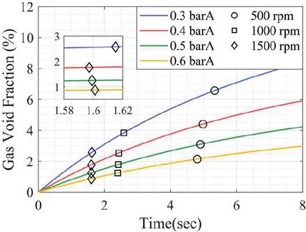
Figure 7 Void fraction predicted with 1st-order air release (, ).
Evident trends from the figure are: more air is released with time progressing; for a specific pressure, the rate of air release slows down with time; and the lower the pressure, the more air is released after the same amount of time. It should also be mentioned that if the pressure change caused by the air release is neglected, the air release process in the fluid that travels along the hydraulic lines can be predicted with constant-pressure curves given in Figure 7. Indeed, the inlet pressure change along the pipe was found to be low, as Figure 8 shows.
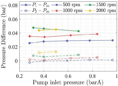
Figure 8 Measured inlet line pressure change (P: pipe enter, P: pipe end).
Apparently, the choice of affects the calculation in Equation (6): higher slower the air release, and it was noticed that a s provides the best consistency with experiments. Specifically, the markers in Figure 7 highlight the predicted gas void fractions at the middle length of the hydraulic line (middle between HL1 and HL2). The predicted GVF values are found to be consistent with the measured GVFs shown in Figure 6. Certain errors in the low GVF region can be explained by the 1st-order being less accurate when the GVF is low, as a smaller bubble size hinders the air release process.
It is worth mentioning that computing the fluid travel time for the markers in Figure 7 involved two counter-acting considerations. On one hand, there is the compressibility-accelerate effect: air release along the pipe causes density to decrease, and to fulfil mass conservation, the flow is accelerated. The flow travel distance L after time t can be determined based on the void fraction history in the fluid element, as Equation (7) gives by assuming the fluid starts from a location where no air is released. Note that the mean flow velocity can be calculated based on the measured flow rate. This mean velocity is considered to happen at the starting location of the hydraulic pipe, assuming the density variation at the position to be negligible due to a minimal air release.
| (7) |
On the other hand, the incomplete-filling-decelerate effect also affects the evaluation of the travel time, where since a lower inlet pressure promotes incomplete filling, the mean velocity which is calculated from the measured flow rate drops, thus giving a longer time for the fluid to reach the same distance. It was observed that such the incomplete-filling-decelerate effect wins over the compressibility-accelerate effect for 500 and 1000 rpm, explaining why for these speeds, the travel time for the fluid to reach the middle of the hydraulic lines becomes longer when the pump inlet pressure decreases. For 1500 rpm, on the other hand, Figure 7 shows that as the pressure decreases, the travel time first decreases and then increases. Such behavior is caused by a weaker incomplete-filling-decelerate effect under 1500 rpm, which loses its dominance to the compressibility-accelerate effect in higher pressure ranges.
Using the software Simerics MP+, CFD simulations were conducted as well to study the dynamic air release process in hydraulic pipes with sub-atmospheric pressure levels. To produce the scenario where an orifice creates the required pressure loss, the considered fluid domain consists of a 3-section cylindrical geometry, an inlet domain, a sharp-edge orifice tube, and an outlet domain, as Figure 9 illustrates (not to scale). The geometry is simulated with static pressure boundary conditions at locations upstream () and downstream () the orifice. The orifice geometry might be differently defined to only include the converging section, as Singhal [18] showed, or to involve chamfers as Zhang et al considered [31] or other more general shapes in Simpson and Ranade [32]. For the purpose of validating the CFD approach, however, the sharp-edge orifice tube is considered.
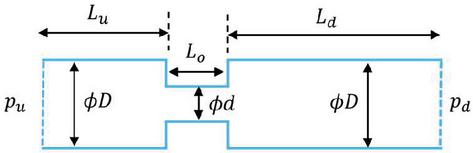
Figure 9 Cross section of the CFD computational domain.
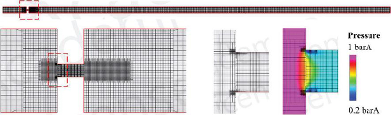
Figure 10 CFD mesh and pressure contour of Orif4.0 when barA.
The geometry of the CFD domains is intended to be designed to replicate the experimentally investigated flow rate conditions. Apparently, different pump operating speeds deliver different flow rates. To reproduce the same pressure drop across the orifice for different flow rates thus requires the orifice to be differently sized. For this consideration, two orifice geometries, referred to as geometry Orif2.8 and Orif4.0 (orifice diameter 2.8 mm and 4 mm) were investigated. These two orifice geometries are expected to deliver 3.4 L/min and 6.8 L/min for the setting of ( barA, barA), i.e., the measured flowrates when the reference positive displacement pump operates at 500 rpm and 1000 rpm (see Figure 4).
Detailed fluid domain dimensions and simulation settings are reported in the appendix. The computational mesh for the geometry Orif4.0 is shown in Figure 10, for example, where increased mesh density is considered in the region close to the orifice and around the orifice inlet edge where high pressure gradient was observed. Mesh cell number for Orif2.8 and Orif4.0 are 800k and 550k, respectively.
As detailed in appendix, CFD simulations of both gas-equilibrium and gas-dissolved fluid models were conducted. It was indeed noticed that the choice of fluid model greatly affects the gas dissolution downstream the orifice, as Figure 11 shows. In the figure, the gas-equilibrium CFD predicted instant air-release at the beginning of the outlet pipe, whereas the gas-dynamics CFD (both steady state simulations) predicted a dynamic air release as the fluid travels along the length of the outlet pipe. The figure compares for the CFD results of the geometry Orif4.0 with outlet pressure 0.4 barA, where the gas-dynamics contour was predicted by air release time constant of 4 s. Notice 0.4 barA produces 4.2e-5 undissolved gas mass fraction for the equilibrium fluid state (total 7e-5), which was instantly reached at the orifice exit for the equilibrium simulation.
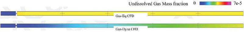
Figure 11 Undissolved gas mass fraction predicted by different fluid models.
On the other hand, however, the flow velocity across the whole computational domain and the pressure distribution at the pump inlet almost do not change between the choice of the two fluid models. As Figure 12 shows. It was found that the CFD-predicted flow rate along the pipe also remains the same for the two types of fluid model (gas-equilibrium and gas-dynamics).
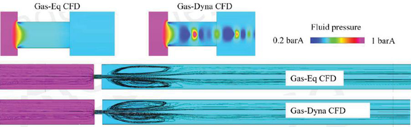
Figure 12 Pressure and streamline comparison between fluid models.
The unchanged flow rate across the orifice indicates a practical way of validating the simulation configuration (geometry, mesh, and fluid) being to reproduce the curves available from literature, especially for low outlet/inlet pressure ratios (). To fulfill this purpose, a separate geometry (noted as OrifVali) that replicates experiments-available literature was investigated. Detailed simulation setting as well as dimensions of this geometry can be found in the appendix. The comparison of the flow across the orifice and measurement results are given in Figure 13, where the pressure ratio is calculated with gauge pressure values. CFD results confirmed that the defined mesh resolution as well as the simulation approach is capable to reproduce the orifice flow features, including the cavitating chocking regime down to very low-pressure ratio.
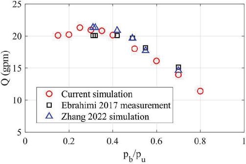
Figure 13 Predicted orifice volume flow validated with measurements in Ebrahimi [33] and simulations by Zhang [31].
To study the dynamic air release process with CFD, the geometry Orif2.8 and Orif4.0 were investigated with the simulation software Simerics, using the dissolved air model as the fluid cavitation model. Key parameters involve the total amount of dissolved gas (mass fraction), the corresponding saturation pressure, and the respective time constants for the air-release and air-absorption process. Detailed CFD settings can be found in the appendix.
The undissolved gas volume fraction results predicted by CFD are plotted in Figures 14 and 15, for geometry Orif2.8 and Orif4.0 respectively. The computational domains are horizontally scaled for plotting convenience. From the figure, certain qualitive observations can be made. First, a lower time constant setting for the air-release in the CFD simulation leads to a faster air-release process. Meanwhile, a lower outlet pressure sees a more severe pressure release process, which can be explained by the increased amount of undissolved gas for the equilibrium state. Last but not least, by comparing between Figures 14 and 15, the high flow rate and thus the faster mean flow velocity downstream the orifice produced by the geometry Orif4.0 shortens the time that the flow takes to travel through the pipe and thus suppresses the amount of undissolved air for the same location under the same pressure settings.
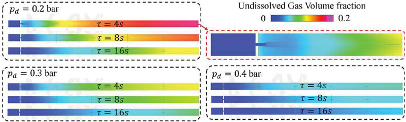
Figure 14 Undissolved gas volume fraction predicted by CFD for Orif2.8.
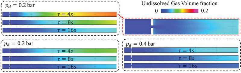
Figure 15 Undissolved gas volume fraction predicted by CFD for Orif4.0.
To quantitatively study the CFD results of the transient air release process, the undissolved gas volume fractions at different locations (grey “+” markers in figure 11) along the pipe downstream the orifice were investigated. Indeed, the value predicted by CFD are compared with the analytical evaluations, i.e., values predicted by Equations (2) (7). Note that because the CFD simulation is isothermal, the polynomial coefficient to be used in Equation (3) is set to be 1. Meanwhile, because the software Simerics assumes that the dissolved gas is fully released at as 0 barA, in Equation (2), is set to be 0 barA for the evaluations to be studied. The comparison between CFD and 1st-order gas dynamic predictions of gas void fractions along the pipe is plotted in Figure 16.
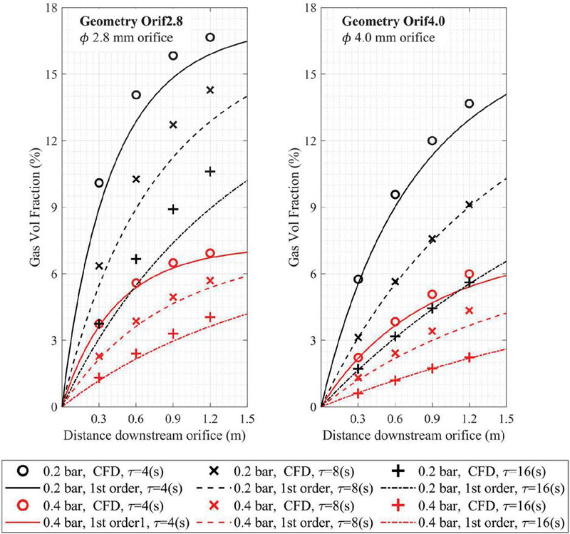
Figure 16 Undissolved gas volume fraction predicted by CFD and 1st-order approach.
In Figure 16, the consistency between the increasing trend and the order of magnitudes between CFD results (markers) and analytical evaluations (curves) re-confirmed the practical use of the 1st-order gas-release evaluation proposed in Section 3.2: the proposed analytical evaluation can practically estimate the amount of the released gas, avoiding CFD simulations which demand additional computational resources. The error between the CFD and analytical results plotted in the diagrams in Figure 16 is found related to flow regime near the orifice exit. As indicated from Figure 14, at the starting point of the downstream pipe, the fluid with 0 undissolved gas only presents in a small volume where the jet flow exists. This flow regime causes (i) additional radial undissolved gas convection to enhance the air-release process along the jet (whereas the analytical evaluation neglects convection effects) (ii) the spatial average of the undissolved gas volume nearly downstream the orifice exit being higher than 0, which was assumed in the analytical evaluations. Note that such flow behavior is attenuated in Figure 15 for the bigger orifice geometry, which explains the less discrepancy between the CFD and analytical evaluation of the Orif4.0 in Figure 16.
The reference pump tested is a crescent-type internal gear pump with involute type gear profiles. To study the pump incomplete filling behavior, isothermal lumped parameter-based pump simulations based on the circuit shown in Figure 17 were performed, considering the fluid with the equilibrium fluid model. In the simulation, the outlet pressure uses the measured values. The simulation model is a simplified version of a more complex model from the authors’ previous work [34]. Particularly, the model used here neglects the viscous leakage in the fluid films and across gear tips, since the outlet pressure was low. Radial micro-motion on the gear set was considered, as it affects the gear center distance and, hence, the effective displacement. The micro-motions of the two gears are solved based on the Ocvirk solution [35], considering both hydrostatic and contact loadings on the gear set [34]. More details on the coupled pump simulation model can be found in the authors’ previous works [34, 36].
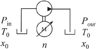
Figure 17 Simulated circuit.
The pump was simulated up to 6 shaft revolutions, and the outlet flow rate averaged from the last 3 gear teeth period was considered to study the incomplete filling behavior. With such a time window, all performed simulations reported an absolute residue of less than 0.02 % in the volumetric efficiency. More details on the simulation settings can be found in Table 2.
| Sim. Setting | Value |
| Fluid | ISO-VG46 |
| 0.22 bar absolute | |
| 1 atm | |
| 23C |
The pump volumetric efficiencies predicted by the simulation model considering different total air settings are compared with the measurements in Figure 18 for the four measured operating speeds.
Figure 18 shows a significant trend: for low speed (500 rpm) and low inlet pressure (0.3, 0.4 bar absolute), a higher total air gives a more accurate prediction in the impaired volumetric efficiency. When the inlet pressure is not very low (0.6 bar absolute), low total air simulation gives better predictions. The trend also appears for 1000 rpm as the figure shows, whereas for higher speeds 1500 rpm and 2000 rpm, this trend was not observed. Instead, for the high speeds, simulation with very low total air appeared to match best with the measured volumetric efficiencies.
The underlying physics in different total air settings can be understood as follows. Due to the equilibrium fluid assumption, when the fluid pressure is below saturation, more air is released into a fluid if the fluid is defined with a higher total air. The higher amount of undissolved air leads to a lower bulk modulus of the fluid mixture, hence giving more density drops when the volume expansion happens inside the pump inlet and consequently a lower volumetric efficiency. On the other hand, the fact that such a trend is not evident for high speeds (1500, 2000 rpm) is that not much air was released for the speeds, which can be confirmed with the measurements in Figure 6.
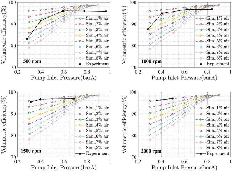
Figure 18 Measured pump volumetric efficiency compared with simulation results predicted based on fluids with different total air values.
As mentioned in Section 2.3, Rundo et al. [14] and Corvaglia et al. [9] once noticed that for the same sub-atmosphere inlet pressure, the higher the operating speed, the more severe the incomplete filling becomes. Actually, such speed dependency can be reproduced from the simulation model used in this paper as well, as Figure 19 shows: for a certain total air, the pump volumetric efficiency drops with a higher speed, indicating a more severe incomplete filling. This speed dependency observed by earlier researchers can be explained as follows. As the flow rate becomes substantially high, the time for air release to happen becomes trivial such that only a very tiny amount of air can be released into the fluid before the pump inlet. Because the volume expansion process in the displacement chamber happens much faster ( s) than the air release process ( s), the fluid that enters the pump, which is off-equilibrium (concerning the air release process), will not change its offequilibrium status during the volume expansion stage. Such behavior gives a good rationale for considering the off-equilibrium fluid at the pump inlet as an equivalent fluid with less total air in the state of air-release equilibrium. In this way, for high-speed operations, the equivalent fluid that enter the pump inlet can be considered as not changing between different operating speeds, as they all equivalently contain a very small amount of total air. In this situation, therefore, the primary cause of the incomplete filling becomes the pressure drop inside the gear displacement chambers, which is related to the volume expansion. Since a higher speed raises the expansion rate, a higher pressure drop can be expected in the displacement chambers and hence increases the volumetric loss for a higher operation speed.
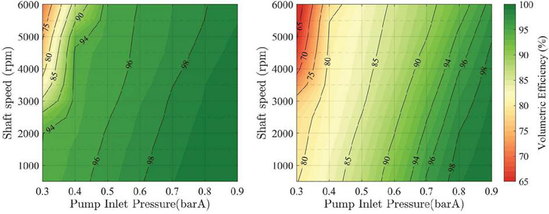
Figure 19 Simulated volumetric efficiency of a wider speed range (left: with 2% total air, right: with 8% total air).
The reason why such speed dependency seems to be reversed for lower speeds (see discussion in Section 2.3) is as follows. A lower speed operation gives the fluid more time to release air; hence, the equivalent fluid that enters the pump inlet at low speeds has a significantly higher amount of total air when compared to the equivalent fluid at high speeds. This means that for a specific inlet pressure where incomplete filling happens, the pump volumetric efficiency should first increase and then decrease. Take 0.3 bar absolute pump inlet pressure shown in figure 19 as an example, when the speed increases from 500 rpm to 2000 rpm, the volumetric efficiency of a pump that is under incomplete filling condition should be first referred to a volumetric efficiency map predicted with a higher total air (e.g., 8 % in the right figure, where a low volumetric efficiency would be found) and then a map with a lower total air (e.g., 2% in the left figure, which gives a higher volumetric efficiency compared to the 8% map for the same speed). In the low-speed domain, the difference in the amount of air that is released into the upstream fluid is the main driving force in determining the incomplete filling, because the fluid compressibility upstream the pump inlet significantly varies in this speed domain. As the operating speed increases from 2000 rpm to higher, the map from where an accurate volumetric efficiency can be found gradually converges towards a map predicted with a trivial amount of total air (e.g., 2 % in the left figure), so that a higher speed gives a lower volumetric efficiency, due to a higher pump internal pressure drop becoming the dominant force in defining the incomplete filling phenomenon.
The fluid at the pump inlet may carry a higher volume of released air than the measured value, which is a type of averaged GVF over the complete hydraulic lines. The increase in the GVF between the measured value and the value that should be expected at the pump inlet can be described with a factor. At first thought this factor should be slightly lower than 2 due to the non-linearity shown in Figure 7, but on the other hand, the non-linearity of the speed of sound (based on which the GVF is measured) with the gas presence involves an opposite effect which raises the factor. In this work, a factor with the value of 2 was found to report the best matching between the experiment and the analytical evaluation. However, to better quantify this factor, a more rigorous evaluation may be desired in future relevant work based on CFD approaches.
In this way, the total air in the equivalent fluid at the pump inlet can be evaluated by back calculating from with a pre-known GVF value. Indeed, by taking as 1, Equation (6) gives the volume of the undissolved gas at the test pressure; and from there using Equation (3) the undissolved gas volume at the reference state can be evaluated; finally with Equation (2) the value of can be found. In this calculation, twice the measured GVF (because of the averaging factor of 2 mentioned earlier, viewed as the GVF at the pump inlet) is used for calculating the value in the first calculation step. Additionally, this three-step calculation bridging between the pump inlet GVF (under certain inlet pressure) and the equivalent total air entering the pump is given with curves plotted in Figure 20, from where the back-calculation can be conveniently looked up. Note that twice the GVF measurements are desired to be used for indexing from the curves in Figure 20.
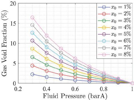
Figure 20 Equilibrium-state gas void fraction in sub-atmospheric fluids with different total airs.
The total air in the equivalent fluid calculated from the measured GVF results is plotted in 21, labelled as “measured equivalent” total airs. Also plotted in Figure 21 are the “simulation proposed” total airs: the total air that gives the best volumetric efficiency predictions from the simulation which can be inferred from Figure 5. To account for possible inaccuracy in volumetric efficiency evaluations under higher inlet pressure conditions (0.6 bar absolute), the “simulation proposed” total air is picked as 0.5 % in the higher pressure range. The comparison in Figure 21 gives a significant consistency between the “measured equivalent” and “simulation proposed” total air. Such consistency once again supports the validity of the gas void fraction measurements and also supports the earlier assumption stating that off-equilibrium fluid entering the pump inlet can be equivalently viewed as a fluid with a lower total air under the equilibrium state.
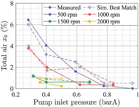
Figure 21 “Measured equivalent” versus “simulation proposed” total air.
Another important consideration can be made from Figure 21: the total air setting in pump incomplete filling simulations is an important and uncertain parameter that should be carefully considered based on the inlet circuit design. For higher flowrates or shorter inlet lines where less air release is expected, a lower total air might be accurate; however, when the air release upstream the pump is not negligible, the total air setting greatly affects the accuracy in predicting the incomplete filling behavior. Notably, this work not only identified the importance of the total air parameter but also for the first time measured its physical value in incomplete filling studies. This breakthrough suggests a promising direction for conditioning the inlet settings in future studies on positive displacement pumps, whether in simulation or tests.
This paper presented a study on the incomplete filling phenomenon of a positive displacement pump.
The study first experimentally investigated the reference pump incomplete filling under different inlet pressure and speed conditions. The measurements were achieved via a novel test rig setup in the authors’ research lab, where two stages of pressure drops, including an upstream orifice and the pump internal inlet pressure drop, were simultaneously investigated. The measurement setup highlights an in-line gas void fraction measurement, the first time for an incomplete filling study to measure the fluid property that enters the pump inlet.
Measurements showed clear signs of incomplete filling when the pump inlet was subject to sub-atmosphere pressures. The measurements unveils the two factors that influence the incomplete filling characteristics of a pump:
(1) In the low speed operating domain, the amount of air released into the fluid upstream the pump inlet is the main driving force in determining the incomplete filling, as the fluid compressibility significantly varies in this speed domain. Since a lower speed gives more time for the air to release into the fluid before the pump inlet, a lower speed leads to a more severe incomplete filling.
(2) In the high speed operating domain, the pump inlet fluid contains a very small amount of undissolved air, so that the fluid compressibility becomes less important. Instead, the higher volume expansion rate inside the pump displacement chambers leads to a higher pressure drop in the displacement chambers, which predominantly defines a more severe incomplete filling situation.
This study also utilized simulations to study the incomplete filling behavior, involving a transient 1st-order air release model to investigate the air release process in the pipe, a CFD-based study of the pipe air release, and an equilibrium-fluid-based LP pump simulation model to investigate the pump’s volumetric performance under incomplete filling.
The 1st-order air release model with 6% total air and 8 second air release time constant showed a good accordance with the measured gas void fraction, supporting the validity of both the model and the gas void fraction measurements in studying the air release process in hydraulic lines.
The 3D-CFD model of an orifice-restricted sub-atmospheric pipe flow was established to study the air release along the pipe flow. The model was validated with available literature reference as per the simulated flow rate under low (0.2 0.4) outlet/inlet pressure ratios. The CFD results showed that (i) the choice between the gas-equilibrium or the gas-dynamic fluid model leads to a major difference in the prediction of the air-release process downstream the restricting orifice, while creating minor changes in the pressure and velocity solution of the flow. (ii) gas-dynamic fluid model simulations produced a consistency for predicting the trends and the order of magnitudes in the pipe flow transient air release, comparing to the analytical 1st-order gas-release formulation proposed in this work and hence confirmed the validity of the analytical evaluation. The consistency was found for a range of air-release time constants (4 s, 8 s, 16 s) and sub-atmosphere pressure levels (0.2 barA, 0.3 barA, 0.4 barA) for two different sized orifice. (ii) for all the compared conditions the CFD results predicted the amount of air-release slightly higher than the analytical evaluation, which was found related to the exit effect of the orifice flow. The CFD results demonstrated that close the orifice exit, trivial gas-volume-fraction fluid only persists in the center of the orifice jet flow such that the spatial averaged air-release is higher than zero which was assumed by the analytical approach. Meanwhile, the jet flow profile and the side-attached high-air region downstream the orifice created the convection of free gas and enhanced the development of air-release, which was an effected neglected in the analytical evaluation.
Results from the equilibrium-fluid-based LP pump simulation showed that the total air setting greatly affects the prediction of the pump incomplete filling. Specifically, for low-speed low inlet pressure conditions, simulation with higher total air gives more accurate volumetric efficiency predictions. The “equivalent” total air at the pump inlet, derived from the gas void measurement, was found to match well the total air settings that give the most accurate incomplete filling predictions. This finding confirms the importance of the total air and also validates a crucial assumption that a fluid that has not reached air-release equilibrium at the pump inlet can be equivalently considered as a different fluid with less total air in the state equilibrium, and they can give the same effective prediction for the incomplete filling phenomenon. Notably, this work not only identified the importance of the “equivalent” total air concept but also measured it for the first time in incomplete filling studies. This finding suggests a promising direction for conditioning the inlet settings in future studies on positive displacement pumps.
The authors would like to thank Prithvi Chandiramani, Seshan Suresh, and David Johnson for the inspiring discussions and valuable technical advice.
In the software Simerics MP+, the module of flow, turbulence, and cavitation were involved, for which the residue convergence level were all set to 1e-3. For all simulations the standard k- turbulence model was used (with the five comprehensively empirical constants [37]).
Table 3 Fluid domain geometries of CFD simulations
| Dimensions | Orif2.8 | Orif4.0 | OrifVali |
| (mm) | 2.8 | 4 | 6.35 |
| (mm) | 5.6 | 8 | 12.7 |
| (mm) | 100 | 100 | 285 |
| (mm) | 1500 | 1500 | 570 |
| D (mm) | 25.4 | 25.4 | 28.5 |
Table 4 CFD simulation settings
| Parameter | Orif2.8, Orif4.0 | OrifVali |
| Fluid | hydraulic oil | water [33] |
| Density () | 875 | 998 |
| Bulk modulus (bar) | 16000 | 21500 |
| Temperature (K) | 300 | 300 |
| Kin. viscosity (cSt) | 46 | 0.55 |
| Cavitation model [38] | Gas-dissolved | Gas-equilibrium |
| (s) | 4,8,16 | N/A |
| (s) | 30 | N/A |
| Total gas mass fraction | 7e-5 | 0 |
| Vapor pressure (barA) | 0.01 | 0.179 |
| (bar gauge) | 0 | 20 |
| (bar gauge) | 0.8, 0.7, 0.6 | 16,14,12,10,8,7,6,5,4,3 |
[1] P. Casoli et al. Modelling of fluid properties in hydraulic positive displacement machines. Simulation Modelling Practice and Theory (2006). https://doi.org/10.1016/j.simpat.2006.09.006.
[2] H. Murrenhoff and K. Schmitz. Fundamentals of Fluid Power. Vol. 7. Reihe Fluidtechnik. Aachen: Shaker Verlag, 2018. isbn: 9783844063066.
[3] J. Ivantysyn and M. Ivantysynova. Hydrostatic Pumps and Motors: Principles, Design, Performance, Modelling, Analysis, Control and Testing. Tech Books International, 2003. isbn: 81-88305-08-1.
[4] A. Vacca and G. Franzoni. Hydraulic fluid power: fundamentals, applications, and circuit design. John Wiley & Sons, 2021. isbn: 978-1-119-56910-7.
[5] P. H. Schweitzer. Effect of Aeration on Gear-Pump Delivery and Lubrication Ceiling. Transactions of the American Society of Mechanical Engineers (1945). https://doi.org/10.1115/1.4018189.
[6] Siemens PLM Software Inc. Simcenter Amesim software User’s guides: AHYD Advanced Fluid Properties Technical bulletin no. 117. 2021.
[7] G. Altare and M. Rundo. Computational Fluid Dynamics Analysis of Gerotor Lubricating Pumps at High-Speed: Geometric Features Influencing the Filling Capability. Journal of Fluids Engineering (2016). https://doi.org/10.1115/1.4033675.
[8] T. Hussain et al. A Simulation Study of Lubricating Oil Pump for an Aero Engine. Journal of Mechanical Engineering (JMechE) (2021). https://doi.org/10.24191/jmeche.v18i3.15417.
[9] A. Corvaglia et al. Simulation and Experimental Activity for the Evaluation of the Filling Capability in External Gear Pumps. Fluids (2023). https://doi.org/10.3390/fluids8090251.
[10] P. Fresia et al. CFD Modelling of an Internal Gear Pump for High Viscosity Fluids. International Design Engineering Technical Conferences and Computers and Information in Engineering Conference 2023. https://doi.org/10.1115/DETC2023-111589.
[11] P. H. Schweitzer and V. G. Szebehely. Gas evolution in liquids and cavitation. Journal of Applied Physics (1950). https://doi.org/10.1063/1.1699579.
[12] H. Pleskun, A. Syring, and A. Brummer. Transient chamber filling in rotary positive displacement vacuum pumps. IOP Conference Series: Materials Science and Engineering (2022). https://doi.org/10.1088/1757-899X/1267/1/012016.
[13] H. Boland and L. Shang. An Analysis of Cavitation Phenomena Scalability in Axial Piston Machine. ASME/BATH 2023 Symposium on Fluid Power and Motion Control 2023. https://doi.org/10.1115/FPMC2023-113585.27.
[14] M. Rundo, G. Altare, and P. Casoli. Simulation of the filling capability in vane pumps. Energies (2019). https://doi.org/10.3390/en12020283.
[15] D. Buono et al. Modelling Approach on a Gerotor Pump Working in Cavitation Conditions. Energy Procedia (2016). https://doi.org/10.1016/j.egypro.2016.11.089.
[16] U. Stuppioni et al. Computational Fluid Dynamics Modeling of Gaseous Cavitation in Lubricating Vane Pumps: On Metering Grooves for Pressure Ripple Optimization. Journal of Fluids Engineering (2022). https://doi.org/10.1115/1.4056416.
[17] F.L. Yin et al. Numerical and experimental study of cavitation performance in sea water hydraulic axial piston pump. Proceedings of the Institution of Mechanical Engineers, Part I: Journal of Systems and Control Engineering (2016). https://doi.org/10.1177/0959651816651547.
[18] A.K. Singhal et al. Mathematical Basis and Validation of the Full Cavitation Model. Journal of Fluids Engineering (2002). https://doi.org/10.1115/1.1486223.
[19] K. Kowalski et al. “Experimental Study on Cavitation-Induced Air Release in Orifice Flows”. Journal of Fluids Engineering (2018). https://doi.org/10.1115/1. 4038730.
[20] H.Q. Yang, A.K. Singhal, and M. Megahed. The full cavitation model. Lecture series – Von Karman Institute for fluid dynamics 4 (2005). purchased on 2020 Sept. from VKI store, p. 10.
[21] U. Stuppioni et al. Computational Fluid Dynamics Modeling of Gaseous Cavitation in Lubricating Vane Pumps: An Approach Based on Dimensional Analysis. Journal of Fluids Engineering (2020). https://doi.org/10.1115/1.4046480.
[22] F. Orlandi, L. Montorsi, and M. Milani. Cavitation analysis through CFD in industrial pumps: A review. International Journal of Thermofluids (2023). https://doi.org/10.1016/j.ijft.2023.100506.
[23] R. Klop, A. Vacca and M. Ivantysynova. A Numerical Approach for the Evaluation of the Effects of Air Release and Vapour Cavitation on Effective Flow Rate of Axial Piston Machines. International Journal of Fluid Power (2010). https://doi.org/10.1080/14399776.2010.10780996.
[24] J. Zhou, A. Vacca, and B. Manhartsgruber. A Novel Approach for the Prediction of Dynamic Features of Air Release and Absorption in Hydraulic Oils. Journal of Fluids Engineering (2013). https://doi.org/10.1115/1.4024864.
[25] Y. G. Shah, A. Vacca, and S. Dabiri. Air Release and Cavitation Modeling with a Lumped Parameter Approach Based on the Rayleigh–Plesset Equation: The Case of an External Gear Pump. Energies (2018). https://doi.org/10.3390/en11123472.28.
[26] Z. Mistry and A. Vacca. Cavitation Modeling Using Lumped Parameter Approach Accounting for Bubble Dynamics and Mass Transport Through the Bubble Interface. Journal of Fluids Engineering (2023). https://doi.org/10.1115/1.4062135.
[27] M. Rundo, R. Squarcini, and F. Furno. Modelling of a Variable Displacement Lubricating Pump with Air Dissolution Dynamics. SAE International Journal of Engines (2018). https://doi.org/10.4271/03-11-02-0008.
[28] Eckerle Technologies GmbH. EIPS segment pump. 2023. url: https://eckerle.com/en/products/eips2-008ra04-1x-s111-eips-segment-pump-industrial-design.
[29] A. B. Wood and R.B. Lindsay. A textbook of sound. 1956.
[30] D. L. Gysling. Accurate mass flow and density of bubbly liquids using speed of sound augmented Coriolis technology. Flow Measurement and Instrumentation (2023). https://doi.org/10.1016/j.flowmeasinst.2023.102358.
[31] Y. Zhang et al. Cavitation optimization of single-orifice plate using CFD method and neighborhood cultivation genetic algorithm. Nuclear Engineering and Technology (2022), https://doi.org/10.1016/j.net.2021.10.043.
[32] A. Simpson and V. V. Ranade. Modelling of hydrodynamic cavitation with orifice: Influence of different orifice designs. Chemical Engineering Research and Design (2018), https://doi.org/10.1016/j.cherd.2018.06.014.
[33] B. Ebrahimi et al. Characterization of high-pressure cavitating flow through a thick orifice plate in a pipe of constant cross section. International Journal of Thermal Sciences (2017), https://doi.org/10.1016/j.ijthermalsci.2017.01.001.
[34] D. Pan and A. Vacca. Total efficiency prediction of crescent type internal gear pump considering floating balancing components. ASME/BATH Symposium on Fluid Power and Motion Control 2023. https://doi.org/10.1115/FPMC2023-111553.
[35] F.W. Ocvirk. Short-bearing approximation for full journal bearings. Tech. rep. NASA Technical Reports NACA-TN-2808, 1952.
[36] D. Pan and A. Vacca. Modeling of crescent-type internal gear pumps considering gear radial micromotion. Chemical Engineering & Technology, special Issue: Digital, Reliable, Sustainable – Recent Innovations in Fluid Power (2022). https://doi.org/10.1002/ceat.202200419.
[37] H. K. Versteeg. An introduction to computational fluid dynamics the finite volume method, 2/E. Pearson Education India, 2007. 29.
[38] Simerics MP+ help document, Physics Modules – Cavitation – Physics – Cavitation Models. Version 6.0.10.

Dinghao Pan, PhD., is currently a research scientist at Maha Fluid Power Research Center at Purdue University. He graduated with his PhD from Purdue University in 2024 with the research focus of developing multi-physics coupled simulation models and numerical methodologies for compensated crescent-type internal gear pumps and external gear pumps. His research interest also involves reduced order tribology modeling and external gear pump modeling.

Andrea Vacca, PhD, is the Maha Fluid Power Faculty Chair and director of the Maha Fluid Power Research Center at Purdue University. The focus of Andrea’s research activities has been fluid power since the beginning of his professional career in early 2000s. Significant research contributions range from modeling techniques for fluid power systems and components, new designs for pumps, as well as principles for enhanced performance of hydraulic control systems.

Venkata Harish Babu Manne, PhD., holds PhD from the Maha Fluid Power Research Center at Purdue University, specializing in Fluid Power, Tribology, and Computational Fluid Dynamics (CFD). With a strong background in research and numerical modeling, Harish has published in Mechanical Systems and Signal Processing and Tribology Transactions. Currently, he is a Project Engineer at Simerics Inc. in Novi, MI, where he applies advanced CFD techniques to solve complex engineering challenges.

Daniel Gysling, PhD., is founder and CEO of CorVera, LLC, a company with a charter to improve the measurement of liquids with entrained gas. Daniel’s technical expertise is in the areas of fluid dynamics and structural dynamics. Daniel holds BS in Aerospace Engineering from The Pennsylvania State University, and a PhD in Aeronautics and Astronautics from the Massachusetts Institute of Technology.
International Journal of Fluid Power, Vol. 26_2, 129–162.
doi: 10.13052/ijfp1439-9776.2622
© 2025 River Publishers