Fast Computation of Hydrodynamic Pressure in Lubricated Contacts: Which Loss is Most Suitable for Physics-Informed Neural Networks Solving the Reynolds Equation?
Faras Brumand-Poor*, Nils Plückhahn, Niklas Bauer and Katharina Schmitz
RWTH Aachen University, Institute for Fluid Power Drives and Systems (ifas), Campus-Boulevard 30, D-52074 Aachen, Germany
E-mail: faras.brumand@ifas.rwth-aachen.de
*Corresponding Author
Received 06 September 2024; Accepted 25 September 2024
Abstract
The frictional behavior of pneumatic seals significantly impacts the functionality of fluid power systems, particularly in fast-switching applications where precision and responsiveness are critical. However, the complex relationship between component properties and friction often makes experimental characterization infeasible or prohibitively expensive. To address this challenge, the Institute for Fluid Power Drives and Systems (ifas) developed the ifas Dynamic Seal Simulation (DDS), an iterative elastohydrodynamic lubrication (EHL) simulation capable of accurately solving the relevant partial differential equations (PDEs) [3]. Since iterative solvers are computationally intensive, neural networks have been explored as a more efficient alternative. While traditional neural networks offer computational advantages, they often lack the ability to understand the physical context of the systems they model, potentially limiting their accuracy and reliability. Physics-Informed Neural Networks (PINNs) have been introduced to overcome these limitations. PINNs integrate the governing physical laws directly into the training process, allowing them to grasp the system’s physical context. This approach opens up new possibilities, including more robust training and the ability to extrapolate beyond the training domain, thereby providing a more reliable and efficient tool for modeling the friction of seals in fluid power systems. In this paper, a previously validated hydrodynamic PINN framework [8, 9] is utilized to solve a variant of the averaged Reynolds equation across three scenarios: divergent, convergent, and curved gaps. The investigation focuses on four -norm training metrics: , , , and . The results indicate that the commonly used metric is the most suitable for the scenarios examined.
Keywords: Tribology, physics-informed neural networks, elastohydrodynamic lubrication, pneumatic sealing, physics-informed machine learning.
1 Introduction
1.1 Motivation
Lubricated contacts play a pivotal role in the performance and efficiency of most fluid power components, including seals in hydraulic cylinders, pneumatic valves, and functionally critical contacts in pumps. These components rely on the precise management of friction to ensure optimal operation, making understanding lubricated contact dynamics essential for designing and maintaining fluid power systems. The physical behavior of lubricated contacts is complex and influenced by numerous factors such as surface roughness, material properties, lubricant characteristics, and operating conditions. This complexity often renders an analytical solution impractical or even impossible; therefore, simplifications are necessary. The interactions within these systems are governed by nonlinear partial differential equations (PDEs) that usually do not have closed-form solutions. Given the intricacies of these systems, experimental approaches to characterize and optimize the behavior of lubricated contacts are also challenging. Experiments are often time-consuming and costly, requiring extensive resources to cover the wide range of operational conditions encountered in real-world applications. Moreover, the results from such experiments can be difficult to generalize across different systems or conditions, limiting their applicability.
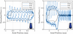
The behavior of lubricated contacts is commonly modeled using elastohydrodynamic lubrication (EHL) simulation, which captures the system’s physics by solving the Reynolds equation to compute the pressure distribution within the lubricating film. A notable example of an EHL simulation model is the ifas DDS, developed to calculate the frictional behavior of reciprocating pneumatic seals. The ifas DDS effectively solves the Reynolds equation to determine the pressure distribution and uses a finite element method (FEM) calculation (Abaqus) to account for the deformation of the seal. This model has been experimentally validated, demonstrating its accuracy in predicting the behavior of seals under various operating conditions (see Figure 1). However, one significant drawback is the computational time required for each iteration [5]. This can become a substantial limitation when multiple iterations are needed or when the model’s complexity increases. One potential solution to reduce the computation time is to increase the available computational power. However, this approach is not always feasible, especially as the complexity of simulations grows. When dealing with multiple contacts or an entire system of contacts, the computational demands can become prohibitively high. In such cases, traditional simulation methods struggle to keep pace, making it almost impossible to calculate these complex interactions within a reasonable time.
This challenge underscores the need for innovative approaches that can maintain the accuracy of traditional EHL simulations while significantly reducing the computational requirements.

Figure 1 Comparison of measured (filtered and unfiltered) and simulated friction force. Left: Without moving over the control edge. Right: Moving over the control edge. [5]
A promising new method developed to address these challenges is the use of Neural Networks (NN). Traditional neural networks are known for their ability to reduce computation time significantly compared to iterative solvers used in distributed simulations. However, this speed comes at a cost. Standard NNs are typically designed to perform regression tasks, where the goal is to minimize the deviation between the predicted output and the actual output. While this approach can produce accurate results within the range of the training data, it cannot understand and incorporate the underlying physical context. As a result, these models may fail to generalize effectively outside the specific data range they were trained on, limiting their applicability in more complex or varied scenarios. Physics-Informed Neural Networks (PINNs) address this limitation by directly incorporating physical laws, such as conservation principles or governing equations like the Reynolds equation in EHL, into the training process. This integration allows PINNs to produce solutions that are not only faster but also more universal, as they are guided by the fundamental physics of the system rather than solely by data-driven correlations. By embedding these physical constraints, PINNs can extrapolate beyond the training data, offering a more robust and accelerated solution that retains the accuracy of traditional methods while overcoming their computational drawbacks. The physics-informed loss is usually formulated as a -norm, most commonly the , a widely used metric in data-driven machine learning. Prior research on this norm for PINNs has suggested that using a different order might lead to improved results [42]. In this paper, we employ a previously validated hydrodynamic PINN framework [8, 9] to solve a variant of the averaged Reynolds equation across three different scenarios: divergent, convergent, and curved gaps. Four training metrics are investigated: , , , and .
In the following sections, 1.2 and1.3, an introduction to hydrodynamic lubrication (HL) and PINNs is provided. Section 2 presents the HD-PINN framework, the physics-informed loss, the training procedure, and the investigated error metrics and scenarios. Section 3 compares the different metrics and validates the results with a variant of the ifas-DDS, referred to as the rigid DDS, which solves the hydrodynamic aspect of an EHL simulation. Finally, Section 4 summarizes the findings and conclusions of this work.
This paper was originally published in the Proceedings of the 14th International Fluid Power Conference [8] and is now extended with novel implementations and results.
1.2 Hydrodynamic Lubrication
EHL simulations are essential tools for evaluating the performance of lubricated contacts, particularly in terms of friction, leakage, and wear characteristics. These simulations take into account the complex interactions between the lubricant and the contacting surfaces, enabling a detailed analysis of how these factors influence surface deformation and the subsequent build-up of hydrodynamic pressure.
The ifas-DDS is a sophisticated simulation model developed to analyze the interactions between a seal and its adjacent counterface. This model explicitly considers the lubrication film that forms between the seal and the counter surface. The deformation of the seal is calculated using the finite element software Abaqus, while HL within the system is described by the Reynolds equation, which governs the pressure distribution in the lubricant film. This equation is seamlessly integrated into the Abaqus environment through a custom subroutine.
The primary focus of this study is the solution of the Reynolds equation without considering the effects of deformation. A modified version of the ifas-DDS model is employed to validate the findings, which does not account for seal deformation either. This version is subsequently referred to as the “rigid DDS”.
Both the rigid and full versions of the ifas-DDS solve an extended form of the Reynolds equation. The originally derived equation from Osbourne Reynolds in 1886 is extended as follows for its usage within ifas DDS [4]:
| (1) |
The Reynolds equation models the hydrodynamic pressure within a narrow lubricated gap. This pressure, which is a function of both position and time , is influenced by several factors: the relative velocity between the surfaces, the fluid’s density , the gap height , the viscosity , as well as the derivatives of pressure with respect to time and position, and . The influence of surface roughness on the hydrodynamics is represented by the pressure flow factor and the shear flow factor , following the averaged flow model by Patir and Cheng [26, 27]. Additionally, the root mean square roughness of the surfaces and the fluid density are considered, though density variations are ignored due to the assumption of an incompressible fluid. This simplifies the Reynolds equation (Equation 1) by dividing through by . The Jakobsson-Floberg-Olsson (JFO) cavitation model is used to accurately describe the behavior of the lubricant in areas where cavitation might occur, introducing the parameter [2]. The cavitation fraction indicates the degree of cavitation within the lubricated contact, which occurs when the pressure drops below the vaporization threshold.
1.3 Physics-Informed Neural Networks
The Reynolds equation, which, as mentioned before, is central to the analysis of lubricated contacts, is traditionally solved using finite volume, finite element, or finite difference methods. These numerical techniques have been well-established in the field of tribology [23, 28] for their ability to provide accurate and detailed solutions. However, recent advances in machine learning have opened up new possibilities for solving these complex equations more efficiently and potentially faster.
Several machine learning models have been developed in the context of tribology, showing promising results. Notable examples include the application of autoencoders and convolutional neural networks (CNNs) for fault detection in tribological systems. These models can identify and diagnose issues in real time, which is critical for maintaining the reliability and performance of mechanical systems.
The work by Hess and Shang [17], who demonstrated the use of a convolutional neural network to determine the elastohydrodynamic pressure distribution in journal bearings is particularly relevant to this study. Their research highlighted the significant potential of machine learning not just for data modeling but also for directly solving PDEs that govern the physical phenomena in tribology.
The theoretical foundation for using neural networks to approximate complex functions, including those described by differential equations, was laid in the late 1980s. In 1989, Cybenko mathematically demonstrated that a feed-forward neural network with at least one hidden layer can approximate any continuous function with arbitrary accuracy, provided the network has sufficient neurons [15]. This result was a significant milestone, establishing the universal approximation capability of neural networks.
In the same year, Hornik extended this proof to Borel measurable functions, further broadening the scope of problems that neural networks could theoretically solve [19]. In 1990, building on these foundational results, Hyuk developed the basic concept of PINNs: his approach involved extending the loss function of a neural network to incorporate the residuals of differential equations [21]. The term “physics-informed” was not used at that time, though.
Despite the early theoretical advancements, the approach of using neural networks to solve differential equations was relatively overlooked. This was mainly due to the computational limitations and the lack of efficient techniques for training neural networks at that time. However, there has been a significant resurgence of interest in PINNs in recent years. This revival can be attributed to several key developments in machine learning and computational technology. First, the exponential growth in computational power, including the advent of powerful GPUs and cloud computing, has made it feasible to train large and complex neural networks. Additionally, machine learning models have become more sophisticated, with improved architectures and training algorithms that can efficiently handle more complicated tasks. Perhaps most importantly, the development of advanced gradient calculation techniques, such as automated differentiation, has dramatically enhanced the ability to compute derivatives accurately and efficiently.
Owhadi, who in 2014 was among the first to reintroduce the idea of using machine learning for solving differential equations, reformulated the problem of solving PDEs as a Bayesian inference problem [25]. Following this, Raissi et al. made significant contributions by developing a probabilistic machine learning algorithm designed explicitly for solving general linear equations using Gaussian processes [31, 32]. Their approach tailored the Gaussian process to fit the structure of PDEs, allowing for an efficient and accurate solution method. Crucially, this methodology was not limited to linear PDEs; they also extended their approach to handle nonlinear PDEs as well [33, 30].
A significant advancement in the field was the introduction of physics-informed machine learning (PIML) [7], which marked a transformative step in how PDEs are solved. Cuomo et al. described this approach as a mesh-free technique for solving PDEs, where the physical laws governing the system are directly embedded into the neural network’s loss function [14].
Raissi and colleagues refined this approach by introducing PINNs as a new class of data-driven solvers. PINNs work by minimizing two critical components within their loss function: the deviation from predefined values, such as boundary and initial conditions (supervised learning), and the residuals of the PDE (unsupervised learning) [34, 35, 29].
The application of PINNs to solve the Reynolds equation has seen rapid development in recent years. The first notable publication in this area was by Almqvist in 2021, focusing on the general applicability of PINNs for solving the Reynolds equation [1]. Following this pioneering work, more advanced algorithms were developed by Zhao et al. and Li et al., who applied PINNs to solve the two-dimensional Reynolds equation in the specific contexts of linear sliders and gas bearings, respectively [44, 22]. A significant recent advancement was made by Rom, who was the first to solve the Reynolds equation incorporating the Jakobsson-Floberg-Olsson (JFO) cavitation model using a PINN [38]. Building on Rom’s work, Cheng et al. developed a more comprehensive PINN framework capable of solving the Reynolds equation with either the JFO or the Swift-Stieber (SS) cavitation models [13]. As part of their work, they also introduced different multi-task learning methods to balance the various loss terms within the PINN, improving the stability of the learning process. Despite these advancements, a significant amount of manual tuning is still required when applying PINNs to such problems since the existing publications have primarily focused on the PINN methodology itself rather than providing a complete and automated framework. Brumand-Poor et al. tackled common challenges in the development of PINNs in general, especially the manual tuning effort, by implementing a sophisticated framework for solving the Reynolds equation and validated the framework for stationary cases without cavitation for single-case and multi-case interpolation and extrapolation tasks [8, 9].
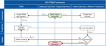
Figure 2 illustrates the architecture of the PINN. The critical components of the PINN are the neural network itself, automatic differentiation, various loss functions, and the optimizer. As part of the overall summed loss, the residual loss contains partial derivatives of the solution with respect to the spatial and temporal variables. To calculate these, the framework employs automatic differentiation. By applying the chain rule, automatic differentiation allows the neural network outputs to be differentiated with respect to the network inputs and its internal parameters, including weights and biases. [10]
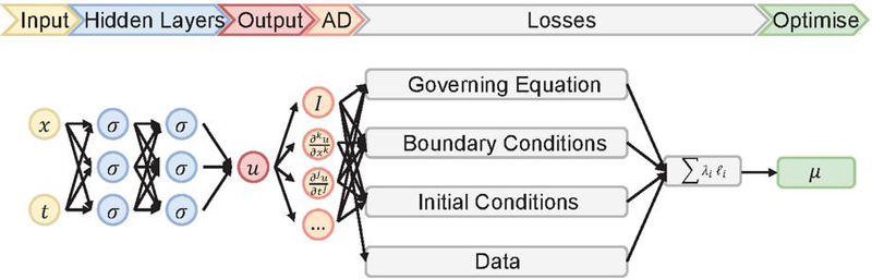
Figure 2 Schematic illustration of a physics-informed neural network [8]
Figure 2 illustrates the different loss components used in the hybrid PINN. The residual loss is derived from the governing equation (e.g. Reynolds equation), ensuring the network’s output adheres to the fundamental physical laws. Boundary and initial condition losses enforce the specific conditions at the seal’s edges and at the initial time along the seal’s length (e.g. for pressure and cavitation). Additionally, if available, a data loss integrates actual or simulated data, such as from the ifas-DDS, to further align the model’s predictions with empirical observations.
Traditional PINNs typically involve three losses: the residual from the governing equation, boundary conditions (BCs), and initial conditions. When an additional data loss is incorporated, the model becomes a hybrid PINN. However, this study focuses on traditional PINNs to explore their potential without integrating external data sources.
Minimizing the three losses is a form of multi-objective optimization, where all loss terms are minimized simultaneously. This approach often conflicts between the different objectives, requiring trade-offs to balance them effectively [11]. The result of this multi-objective optimization can be seen as a set of Pareto optima, where no single objective can be improved without worsening another [40].
While multi-objective optimization is theoretically independent of how these terms are balanced [18], the non-convex nature of the physical solution space introduces significant challenges. Gradient-based optimization methods, commonly used in PINNs, struggle to find globally optimal solutions in such complex domains [7]. The gradients associated with different loss terms can vary significantly. Most optimizers update network parameters using explicit schemes. If these optimization steps are too large, the process can become unstable, leading to poor convergence.
This issue is less pronounced in classical neural networks, where loss gradients usually have more consistent magnitudes. However, in PINNs, the variability in gradient magnitudes necessitates smaller learning rates, reducing the update size in each optimization step. Unfortunately, this can trap the optimizer in local minima, preventing it from finding the global best solution. To address this, a loss balancing algorithm is implemented in the PINN framework used in this study, helping to stabilize the optimization process and improve the likelihood of reaching a satisfactory solution. The loss balancing is presented in Section 2.3.
Training a PINN requires careful selection of several hyperparameters, such as network width, depth, and the learning rate. In the context of multi-objective optimization, additional hyperparameters are needed to configure the loss balancing. Each hyperparameter represents a tuning dimension, making finding the optimal set a complex and iterative process.
The challenge lies in using inappropriate hyperparameters, depending on the specific training case, can lead to non-convergence. Therefore, identifying the correct set of hyperparameters is crucial for successful training. Traditionally, this is done through manual tuning or grid search, but these methods are often inefficient and suffer from the curse of dimensionality [16], where the number of potential hyperparameter combinations grows exponentially with the number of parameters. To address these challenges, the framework presented in this study includes an automated hyperparameter search process, which is detailed in chapter 2.2.
In summary, PINNs show great promise for solving HL simulation models, offering the potential to make predictions without the need for iterative methods. The following section introduces the HD-PINN framework, which incorporates the differential equation of the HL model, along with features like automated hyperparameter search and loss balancing.
2 The HD-PINN Framework
2.1 The Physics-Informed Loss
As mentioned in the previous section, a few researchers have investigated the PINN for solving the Reynolds equation. The researchers focused primarily on solving the equation with a PINN and, therefore, had to manually tune many design options, e.g., layer width or depth. Therefore, in this work, a previously validated HD-PINN framework is used and extended to address the different norms for the physics-informed loss terms. The investigations are performed on a variant of the Reynolds equation. Still, it can be easily extended to the complete mathematical expression with the transient term and the JFO cavitation model. It is based on the following assumptions:
• Time dependencies are neglected ()
• Cavitation is not considered ()
• The surface is ideally smooth (, )
Therefore, the investigated Reynolds equation can be written as:
| (2) |
The PINN’s input parameters are the dynamic viscosity , the gap height , and the velocity of the counter surface and compute the pressure as output. Partial differentials are calculated via automatic differentiation, which allows for accurate and efficient function derivation [6]. The Dirichlet boundary conditions for the Reynolds equation are stated as two individual loss values for the left and right boundary, respectively. These are compared to the PINN’s boundary pressure prediction The physics-informed Reynolds loss is implemented according to the following:
| (3) |
and the boundary loss is implemented as follows:
| (4) |
The -norm is calculated for the different types of losses, whereby one of the most common norms is the for PINNs [42].
In summary, the PINN’s loss incorporates three terms independent of any specific data provided by simulations or experiments. The rigid DDS is solely used to acquire a pressure distribution to validate the PINN. The two main features of the HD-PINN framework are presented in the next section. These improve the previously mentioned common drawbacks occurring during PINN training runs. Lastly, the whole training process is described.
2.2 Hyperparameter Optimization
Due to the loss balancing mentioned above, PINNs exhibit even more hyperparameters than traditional neural networks. Basic approaches for finding optimal parameters often suffer from the curse of dimensionality and are, therefore, not feasible for the HD-PINN framework.
Bayesian optimization [24] offers a solution to this dilemma and has already been successfully integrated into PINNs [16]. It tries to obtain an optimal set of hyperparameters with as few training procedures as possible by approximating an unknown loss function (PINN losses) with a probabilistic surrogate model (Gaussian Process). Once a set of hyperparameters is evaluated, the next set is chosen based on an acquisition function (expected improvement), which tries to achieve a trade-off between exploration and exploitation by comparing the next chosen set to the current best set. The HD-PINN framework incorporates Bayesian optimization to search the optimal hyperparameters. These include the number of layers, layer width, and four different parameters relevant to the loss balancing task: decay rate, learning rate, temperature factor, and saudade value. In the following section, these parameters will be introduced.
2.3 Loss Balancing
Bayesian optimization is performed to find the optimal set of hyperparameters for the given task. The performance of a given set of hyperparameters is analyzed by training the PINN for a predefined number of epochs, and eventually, the final sum of losses is evaluated. The PINN determines the pressure distribution based on the inputs for a predefined number of collocation points (ten in this work) during each epoch. The Reynolds equation’s residual loss and the boundary values loss are determined according to the predicted pressure distribution. The loss is then differentiated with automatic differentiation to calculate the changes in the network parameters (e.g., weights and biases). These network parameters are optimized using the adaptive moment estimation (ADAM) algorithm. ADAM is a first-order gradient-based explicit optimization method for stochastic objective functions [20]. It is widely recognized as one of the state-of-the-art optimizers for deep neural networks [39, 37] and is computationally efficient with little memory requirements, capable of solving problems of large scale, and has successfully been implemented in PINN applications [41].
As mentioned in the previous section, PINNs might face problems in case of heavily varying loss term magnitudes. A loss balancing scheme is added to the HD-PINN framework to stabilize the learning process according to [7]. Bischof proposed an algorithm combining three existing methods and adding a novel feature. These four features of the Relative Loss Balancing with Random Lookback (ReLoBRaLo) are as follows:
1. The sum of scalings is bound by a softmax function, which is adjusted by the so-called temperature factor [36].
2. The learning progress is monitored by dividing the loss at the current iteration by the loss of the last iteration [12].
3. Inspired by the Learning Rate Annealing, the scalings are set to higher values initially and decay exponentially over the iterations with the decay factor . This leads to the utilization of loss statistics from more than one training step [43].
4. A random lookback (defined by the saudade value ) is embedded in the exponential decay and randomly decides whether to consider the previous steps’ loss statistics or to look back to the beginning of the training for computing the scalings [7].
By tackling the loss scaling problems, this novel balancing algorithm significantly improves the HD-PINN framework’s performance. Figure 3 illustrates the training progress of the complete HD-PINN framework. First, the Bayesian optimizer selects parameters, which are used to initialize the PINN and the network parameter optimizer. Afterward, the PINN calculates the actual pressure prediction and the loss is computed. During each epoch, the loss is used to update the PINN’s weights and biases, and a new pressure distribution is predicted. This loop continues until a certain number of iterations is reached. Once the final epoch is reached, the parameter determined by the Bayesian optimizer is updated. In the next section, the whole framework is validated for two different scenarios and illustrates the training progress.
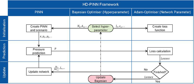
Figure 3 The HD-PINN framework and its training progress. [8]
2.4 The Error Metrics and the Scenarios
This section presents the four different norms for the two types of losses, followed by the three investigated scenarios.
2.4.1 Physics-Informed Losses
In this work, we investigate four different versions of the -norm for the two different loss terms, resulting in eight different equations, seen in Equations 5 to 12. The first norm is the , which represents the mean absolute error regarding the residual and the boundary conditions.
| (5) | |
| (6) |
Secondly, is implemented, which computes the root mean absolute error regarding the residual and the boundary conditions.
| (7) | |
| (8) |
The third norm is the squared norm, , which is a variant of the norm and calculates the mean squared error.
| (9) | |
| (10) |
The last norm is the infinity norm, , which computes the maximum absolute error of residual equation and boundary conditions.
| (11) | |
| (12) |
These different norms are implemented in the HD-PINN training procedure and utilized to solve the following test cases.
2.4.2 Test Scenarios
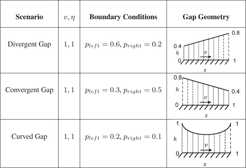
Three different scenarios are investigated. Table 1 illustrates the scenarios, set parameters, and boundary conditions. The difference between the scenarios is the gap geometry, a linear divergent gap in the first case, a linear convergent gap in the second case, and a curved gap in the last case. The training procedure is done for each scenario with each norm, as described in the prior section.
Table 1 Overview of the test scenarios
As described in the previous section, the training procedure was conducted for each scenario using each norm. First, Bayesian optimization was used to tune the hyperparameters over thirty trials. The actual training was then performed with an initial 200 training epochs.
For the and norms, the number of training epochs was increased to achieve a pressure build-up with less than % deviation from the DDS-computed pressure across the entire geometry. Since and are variations of each other, their results were directly compared, with the number of training epochs adjusted based on the norm that required fewer iterations. Notably, epochs were sufficient for in all test scenarios, so the number of epochs for was also set to 200.
3 Results and Discussion
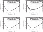
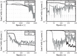
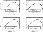
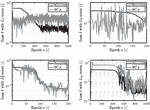
The results are presented and discussed in the following section. First, the pressure build-up is illustrated, followed by a presentation of the specific loss trajectories. The divergent gap is the first scenario in Figure 4. Given the assumption that no cavitation occurs, the pressure can drop below zero. The norm accurately captures the negative pressure build-up within epochs. The loss, depicted in Figure 5, shows a stable decline concerning the residual term and small fluctuations in the boundary conditions.
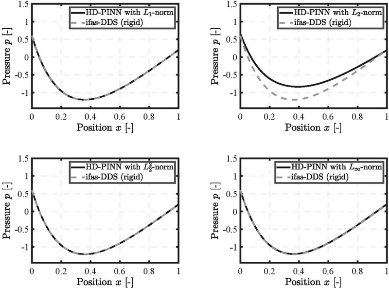
Figure 4 Pressure distribution for the divergent gap using , , and norms trained for epochs, and norm trained for epochs.
However, the norm fails to accurately capture the pressure build-up, particularly within the gap geometry, resulting in errors exceeding %. For the norm, the number of epochs needed to achieve an accurate solution had to be increased to . The norm also produced an accurate solution with the initial epochs. The final loss values vary significantly depending on the norm used, even though the overall performance is similar. Furthermore, the fluctuations are significantly larger for the , and norm compared to , with even exhibiting an increase in the BC loss term.
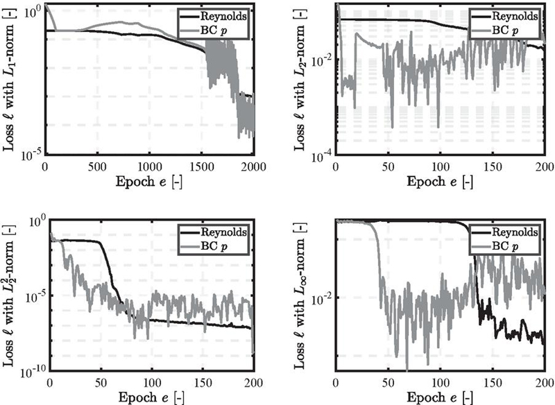
Figure 5 Loss trajectories for the divergent gap.
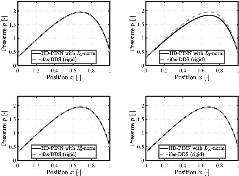
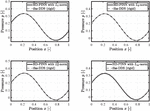
Figure 6 Pressure distribution for the convergent gap using , and , norms trained for epochs, and and norms trained for epochs.
Figure 6 shows the results for the second scenario, the convergent gap. Similar to the divergent gap, the norm successfully trains within 200 epochs, while the norm exhibits deviations in pressure within the gap. However, the error is smaller for the convergent gap, remaining below a maximum of % for each position . As in the first scenario, the boundary conditions are satisfied, and the deviations occur within the gap geometry, attributed to the residual loss term.
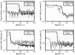
For the and norms, the number of epochs had to be set to 1000. This represents a decrease for compared to the divergent gap and an increase for . Figure 7 illustrates that the different loss trajectories over training align with the results from the divergent gap. The norm shows a declining and stable loss trajectory, with minor fluctuations in the boundary condition loss. The other three norms exhibit more significant fluctuations and a less steady decline, particularly for the boundary condition loss of and .
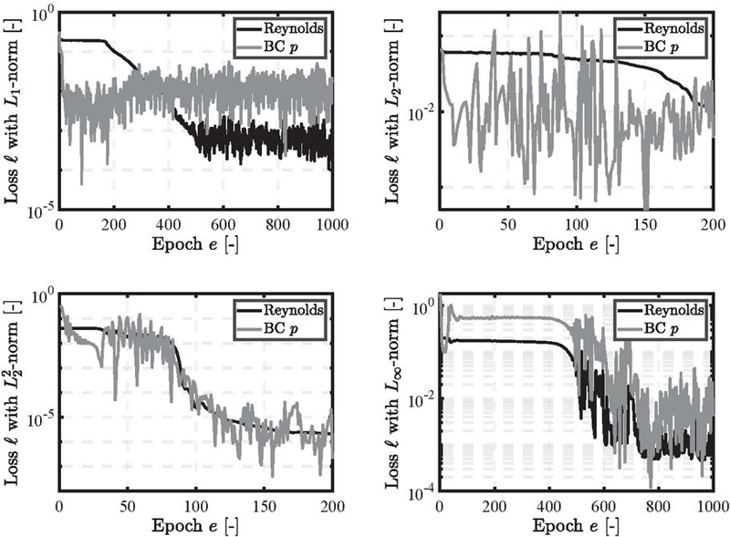
Figure 7 Loss trajectories for the divergent gap.
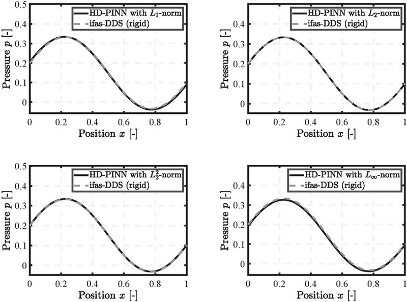
Figure 8 Pressure distribution for the curved gap using , , , and norms trained for .
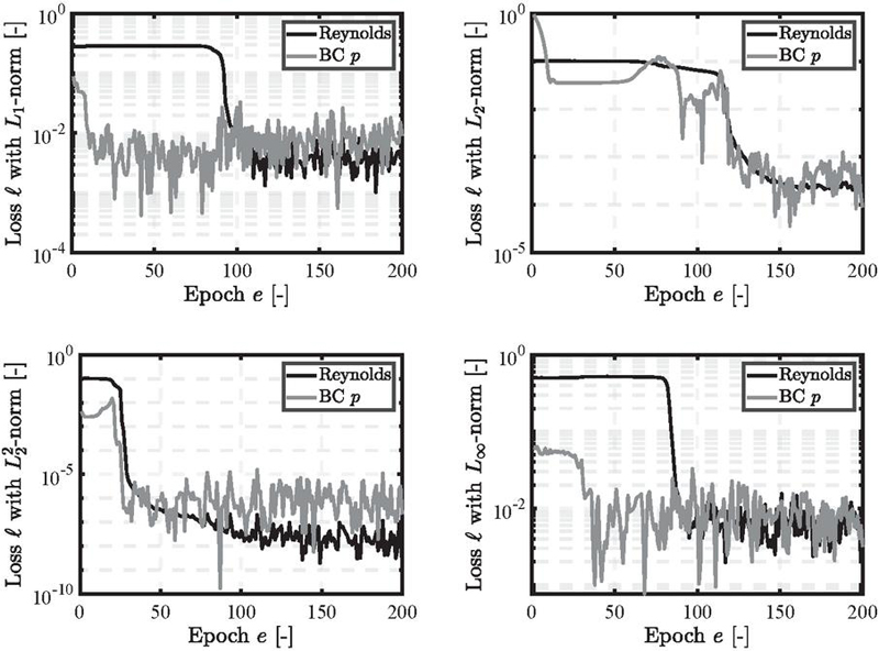
Figure 9 Loss trajectories for the divergent gap.
In the last scenario, the curved gap, the results shown in Figure 8 indicate that all four norms perform well, with slight deviations noticeable in the and norms. However, the overall error remains small and acceptable. Each of the four norms achieved the desired results with the initially set number of 200 epochs, as shown in Figure 9. Each loss trajectory exhibits a declining trend, with the norm showing the earliest decline compared to the other norms. This behavior, observed in the previous loss trajectories, suggests that the norm may achieve reasonable results with fewer epochs. All norms exhibit small fluctuations with comparable amplitudes.
In summary, the best-performing norm out of the four, , , , and , across the three scenarios (divergent, convergent, and curved gaps) is the norm, which exhibits the highest accuracy with the fewest number of epochs and the most stable loss trajectories.
4 Summary & Conclusion
This work applied an automated HD-PINN framework to predict pressure build-up in three test scenarios, divergent, convergent, and curved gaps—based on a variant of the Reynolds equation. To gain a deeper understanding of PINNs, four different -norms, , , , and , were implemented. Each norm was used to solve the three test scenarios and validated against the rigid DDS’s numerical solution. The results highlight that the previously used norm consistently performed the best across all scenarios regarding its accuracy, robustness, and training speed.
Future work will examine the application of these norms to more complex scenarios, including cavitation and transient phenomena, and the implementation of different norm types, such as the Sobolev norm.
Acknowledgement
The authors thank the Research Association for Fluid Power of the German Engineering Federation VDMA for its financial support (grant: FKM No. 7058400). Special gratitude is expressed to the participating companies and their representatives in the accompanying industrial committee for their advisory and technical support.
Biographies
[1] Andreas Almqvist. Fundamentals of physics-informed neural networks applied to solve the reynolds boundary value problem. Lubricants, 9(8):82, 2021.
[2] Julian Angerhausen, Maik Woyciniuk, Hubertus Murrenhoff, and Katharina Schmitz. Simulation and experimental validation of translational hydraulic seal wear. Tribology International, 134:296–307, 2019.
[3] Niklas Bauer, Matthias Baumann, Simon Feldmeth, Frank Bauer, and Katharina Schmitz. Elastohydrodynamic simulation of pneumatic sealing friction considering 3d surface topography. Chemical Engineering & Technology, 46(1):167–174, 2023.
[4] Niklas Bauer, Andris Rambaks, Corinna Müller, Hubertus Murrenhoff, and Katharina Schmitz. Strategies for implementing the jakobsson-floberg-olsson cavitation model in ehl simulations of translational seals. International Journal of Fluid Power, 2021.
[5] Niklas Bauer, Bekgulyan Sumbat, Simon Feldmeth, Frank Bauer, and Katharina Schmitz. Experimental determination and ehl simulation of transient friction of pneumatic seals in spool valves. Sealing technology - old school and cutting edge : International Sealing Conference : 21st ISC, pages 503–522, 2022.
[6] Atilim Gunes Baydin, Barak A. Pearlmutter, Alexey Andreyevich Radul, and Jeffrey Mark Siskind. Automatic differentiation in machine learning: a survey. Atilim Gunes Baydin.
[7] Rafael Bischof and Michael Kraus. Multi-objective loss balancing for physics-informed deep learning.
[8] Faras Brumand-Poor, Niklas Bauer, Nils Plückhahn, and Katharina Schmitz. Fast computation of lubricated contacts: A physics-informed deep learning approach. International Journal of Fluid Power, 19:1–12, 2024.
[9] Faras Brumand-Poor, Niklas Bauer, Nils Plückhahn, Matteo Thebelt, Silas Woyda, and Katharina Schmitz. Extrapolation of hydrodynamic pressure in lubricated contacts: A novel multi-case physics-informed neural network framework. Lubricants, 12(4):122, 2024.
[10] Shengze Cai, Zhiping Mao, Zhicheng Wang, Minglang Yin, and George Em Karniadakis. Physics-informed neural networks (pinns) for fluid mechanics: a review. Acta Mechanica Sinica, 37(12):1727–1738, 2021.
[11] R. Caruana. Multitask learning. Machine Learning, 1997.
[12] Zhao Chen, Vijay Badrinarayanan, Chen-Yu Lee, and Andrew Rabinovich. Gradnorm: Gradient normalization for adaptive loss balancing in deep multitask networks. 2018.
[13] Yiqian Cheng, Qiang He, Weifeng Huang, Ying Liu, Yanwen Li, and Decai Li. Hl-nets: Physics-informed neural networks for hydrodynamic lubrication with cavitation. Tribology International, 188:108871, 2023.
[14] Salvatore Cuomo, Vincenzo Schiano Di Cola, Fabio Giampaolo, Gianluigi Rozza, Maziar Raissi, and Francesco Piccialli. Scientific machine learning through physics–informed neural networks: Where we are and what’s next. Journal of Scientific Computing, 92(3), 2022.
[15] G. Cybenko. Approximation by superpositions of a sigmoidal function. Mathematics of Control, Signals, and Systems, 2(4):303–314, 1989.
[16] Paul Escapil-Inchauspé and Gonzalo A. Ruz. Hyper-parameter tuning of physics-informed neural networks: Application to helmholtz problems.
[17] Nathan Hess and Lizhi Shang. Development of a machine learning model for elastohydrodynamic pressure prediction in journal bearings. Journal of Tribology, 144(8), 2022.
[18] A. Ali Heydari, Craig A. Thompson, and Asif Mehmood. Softadapt: Techniques for adaptive loss weighting of neural networks with multi-part loss functions.
[19] Kurt Hornik, Maxwell Stinchcombe, and Halbert White. Multilayer feedforward networks are universal approximators. Neural Networks, 2(5):359–366, 1989.
[20] Diederik P. Kingma and Jimmy Ba. Adam: A method for stochastic optimization.
[21] Hyuk Lee and In Seok Kang. Neural algorithm for solving differential equations. Journal of Computational Physics, 91(1):110–131, 1990.
[22] Liangliang Li, Yunzhu Li, Qiuwan Du, Tianyuan Liu, and Yonghui Xie. Ref-nets: Physics-informed neural network for reynolds equation of gas bearing. Computer Methods in Applied Mechanics and Engineering, 391:114524, 2022.
[23] Max Marian and Stephan Tremmel. Current trends and applications of machine learning in tribology—a review. Lubricants, 9(9):86, 2021.
[24] J. Močkus. On bayesian methods for seeking the extremum. In G. Goos, J. Hartmanis, P. Brinch Hansen, D. Gries, C. Moler, G. Seegmüller, N. Wirth, and G. I. Marchuk, editors, Optimization Techniques IFIP Technical Conference Novosibirsk, July 1–7, 1974, volume 27 of Lecture Notes in Computer Science, pages 400–404. Springer Berlin Heidelberg, Berlin, Heidelberg, 1975.
[25] Houman Owhadi. Bayesian numerical homogenization.
[26] Nadir Patir and H. S. Cheng. An average flow model for determining effects of three-dimensional roughness on partial hydrodynamic lubrication. Journal of Lubrication Technology, 100(1):12–17, 1978.
[27] Nadir Patir and H. S. Cheng. Application of average flow model to lubrication between rough sliding surfaces. Journal of Lubrication Technology, 101(2):220–229, 1979.
[28] Uma Maheshwera Reddy Paturi, Sai Teja Palakurthy, and N. S. Reddy. The role of machine learning in tribology: A systematic review. Archives of Computational Methods in Engineering, 30(2):1345–1397, 2023.
[29] M. Raissi, P. Perdikaris, and G. E. Karniadakis. Physics-informed neural networks: A deep learning framework for solving forward and inverse problems involving nonlinear partial differential equations. Journal of Computational Physics, 378:686–707, 2019.
[30] Maziar Raissi and George Em Karniadakis. Hidden physics models: Machine learning of nonlinear partial differential equations. Journal of Computational Physics, 357:125–141, 2018.
[31] Maziar Raissi, Paris Perdikaris, and George Em Karniadakis. Inferring solutions of differential equations using noisy multi-fidelity data.
[32] Maziar Raissi, Paris Perdikaris, and George Em Karniadakis. Machine learning of linear differential equations using gaussian processes.
[33] Maziar Raissi, Paris Perdikaris, and George Em Karniadakis. Numerical gaussian processes for time-dependent and non-linear partial differential equations.
[34] Maziar Raissi, Paris Perdikaris, and George Em Karniadakis. Physics informed deep learning (part i): Data-driven solutions of nonlinear partial differential equations.
[35] Maziar Raissi, Paris Perdikaris, and George Em Karniadakis. Physics informed deep learning (part ii): Data-driven discovery of nonlinear partial differential equations.
[36] Aravind Rajeswaran, Chelsea Finn, Sham M. Kakade, and Sergey Levine. Meta-learning with implicit gradients. CoRR, abs/1909.04630, 2019.
[37] Mohamed Reyad, Amany M. Sarhan, and M. Arafa. A modified adam algorithm for deep neural network optimization. Neural Computing and Applications, 35(23):17095–17112, 2023.
[38] Michael Rom. Physics-informed neural networks for the reynolds equation with cavitation modeling. Tribology International, 179:108141, 2023.
[39] Robin M. Schmidt, Frank Schneider, and Philipp Hennig. Descending through a crowded valley - benchmarking deep learning optimizers.
[40] Ozan Sener and Vladlen Koltun. Multi-task learning as multi-objective optimization. CoRR, abs/1810.04650, 2018.
[41] Soumyendra. Singh, Dharminder Chaudhary, B. Yogiraj, Ram Narayan Prajapathi, and Saurabh Rana. Adam optimization of burger’s equation using physics-informed neural networks. In 2023 International Conference on Advancement in Computation & Computer Technologies (InCACCT), pages 129–133. IEEE, 2023.
[42] Chuwei Wang, Shanda Li, Di He, and Liwei Wang. Is physics-informed loss always suitable for training physics-informed neural network?, 2022.
[43] Sifan Wang, Yujun Teng, and Paris Perdikaris. Understanding and mitigating gradient pathologies in physics-informed neural networks.
[44] Yang Zhao, Liang Guo, and Patrick Pat Lam Wong. Application of physics-informed neural network in the analysis of hydrodynamic lubrication. Friction, 11(7):1253–1264, 2023.
Biographies

Faras Brumand-Poor received a bachelor’s degree in electrical engineering from RWTH Aachen University in 2017, a master’s degree in electrical engineering from RWTH Aachen University in 2019, a master’s degree in automation engineering from RWTH Aachen University in 2020, respectively. He is currently working as a Research Associate at the Institute for Fluid Power Drives and Systems at RWTH Aachen University. His research areas include deep learning, physics-based learning, control engineering, fluid transmission lines, and virtual sensory.
Nils Plückhahn received a bachelor’s degree in computer engineering science from RWTH Aachen University in 2023. He is currently working as a Student assistant at the Institute for Fluid Power Drives and Systems at RWTH Aachen University. His research areas include physics-informed machine learning, elastohydrodynamic simulation, and tribology.

Niklas Bauer received a bachelor’s degree in mechanical engineering from RWTH Aachen University in 2017 and a master’s degree in development and design from RWTH Aachen University in 2019, respectively. He is currently working as the Chief Engineer at the Institute for Fluid Power Drives and Systems at RWTH Aachen University. His research areas include lubricated contacts, elastohydrodynamic simulation, and tribology.

Katharina Schmitz received a graduate’s degree in mechanical engineering from RWTH Aachen University in 2010 and an engineering doctorate from RWTH Aachen University in 2015. She is currently the director of the Institute for Fluid Power Drives and Systems (ifas) RWTH Aachen University.
International Journal of Fluid Power, Vol. 25_4, 439–464.
doi: 10.13052/ijfp1439-9776.2542
© 2024 River Publishers