Determination of the Flow Angle in Hydraulic Components

Lennard Günther^*, Sven Osterland and Jürgen Weber

Institute of Mechatronic Engineering, Technische Universität Dresden, Helmholtzstrasse 7a, 01069 Dresden
E-mail: Lennard.guenther@tu-dresden.de
*Corresponding Author

Received 20 September 2024; Accepted 18 October 2024

Abstract

The paper presents a general analytical equation for the determination of the flow angel in hydraulic components like valves and pumps. Exemplary, the method is applied to two different valve concepts – a cartridge valve and a rotary slide valve.

$$\mathit{c}\mathit{o}\mathit{s}({\mathit{\epsilon }}_{\mathit{a}\mathit{v}\mathit{g}})=\frac{\mathbf{1}}{\mathbf{2}}(\mathit{c}\mathit{o}\mathit{s}({\mathit{\alpha }}_{\mathit{l}})-\mathit{c}\mathit{o}\mathit{s}({\mathit{\alpha }}_{\mathit{r}}))$$

The huge advantage of this equation is the simple expression with no dependencies on operation conditions. Only the geometry is important. The underlying phenomenon is valid for turbulent flows. Thus it is useable for almost all hydraulic applications. It makes it possible to predict the flow force as well as to optimize the flow geometry. It describes the flow angle of the free jet behind a narrow section (e.g. a control edge of a valve). By a suitable choice of the angle of the free jet, the flow force can be reduced by changing the direction of the outgoing impulse. With regard to cavitation, the impact of the free jet can be shifted and thus the cavitation erosion can be shifted or weakened.

This paper deals with the investigation of the flow angle of free jets as well as the prediction of the flow force in valves without CFD. For the illustration a cartridge and a rotary slide valve are used as technical applications. In the first section, geometric factors influencing the flow angle are discussed, as well as the transferability of the results under varying operating conditions (laminar and turbulent). Using a generic minimal model, the behaviour of the flow angle with respect to geometric influence factors and operating conditions is investigated by means of CFD. The results are adapted to real applications in the second section. The direct adjustment of the flow angle results in a significant improvement in the characteristic behaviour of the presented valves (such as flow force and resistance torque). It becomes clear how efficient the adjustment of the flow angle can be if the basis of the formation of the free jet is known. Due to the derivation of the relationship with the help of an abstracted minimal model, the knowledge gained can be used in many ways and can also be transferred to other applications in the field of fluid technology. Optimization processes are more efficiently without using elaborated simulation models e.g. driven by CFD.

Keywords: Flow angle, free jet, flow force, hydraulics, design process.

1 Introduction

The flow angle of the free jet plays a decisive role in the functionality and performance of fluid power components. Internal flows, which are common in hydraulics, have a large number of abrupt cross-sectional constrictions. At those narrow points, e.g. at control edges of valves, a free jet is formed as the flow passes through. This free jet influences the resulting flow force acting on the valve spool [1]. In addition, the free jet has a great influence on the formation and transport of cavitation bubbles. In the shear layers of the free jet, vortices are formed in which the bubbles are created and grow [2]. The bubbles are transported with the flow and collapse if the local pressure increases again, e.g. at stagnation points. In areas close to the wall, this leads to a microjet. That causes erosion damage to the component, shown in [1] and [3]. However, free jets also occur in pumps such as the valve plate of an axial piston pump, during the transition from low pressure to high pressure, which can cause cavitation damage [4]. Depending on the geometry, the free jet aligns itself via the flow angle. The literature on specific angle positions is long. In [1], the angle for individual control positions of a spool valve is defined. Similarly, the flow angles are described for example by [5–8], where all data on the angle correlate well with an acceptable scatter. In [9] and [10] the clearance at the valve spool and the sleeve are considered, which is important for very small opening ratios.

A common question during the valve and pump development process is: In what way is the flow angle affected by the control edge geometry? This paper deals with the investigation of the flow angle by using a generic minimal model. The aim is a general method about how the flow angle results from geometric parameters and in which operating range it is valid. The transfer of the results to a real application reflects the applicability of the obtained correlation. The implementation is carried out using two different valve concepts – a rotary slide valve and a conventional cartridge valve. In the first application the calculation of the flow angle is compared with CFD data of the rotary slide valve. The flow angle of the free jet has to be modified to improve the performance of the valve. As reference the evaluation will be done with the flow characteristics (such as resistance torque). The second application – the cartridge valve – will be used to predict the flow force. The very good results of the flow angle calculation make it possible to use the analytical method to calculate flow angle dependent behaviours.

The rotary slide valve is illustrated in Figure 1. As a special design compared to conventional rotary slide valves, this one is integrated into a cartridge installation space. The valve can be operated in both flow directions. The illustration shows for example of the flow direction the inlet horizontally and the outlet vertically on the bottom. The valve has three control edges in the horizontal plane, which are offset by 120${}^{\circ }$. A complete opening and closing process takes place at a twisting angle $\phi$ of 0${}^{\circ }$ (fully open) to 60${}^{\circ }$ (closed).

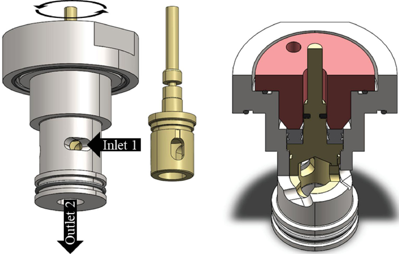
Figure 1 Rotary slide valve, exemplary flow direction $1\to 2$ through the assembly (left), valve spool (middle), sectional view through the inlet plane and the vertical center plane (right).

A conventional cartridge valve is shown in Figure 2. This type of valve has a piston in the shape of a cylinder and as seat geometry a chamfer. The inlet of this valve is vertically on the bottom and the outlet horizontally. The most important part of the valve is the control edge – the cross-sectional area of the flow. It influences almost all characteristics of the valve. The narrow section is formed between the bottom edge of the piston and the geometry of the chamfer. Thus, there are two possible narrow section definitions in this valve configuration. Inside the chamfer (small strokes) it is defined by the chamfer itself. Outside the chamfer (lager strokes) the influence of the chamfer decrease and the upper edge of the chamfer geometry is important for the control edge.

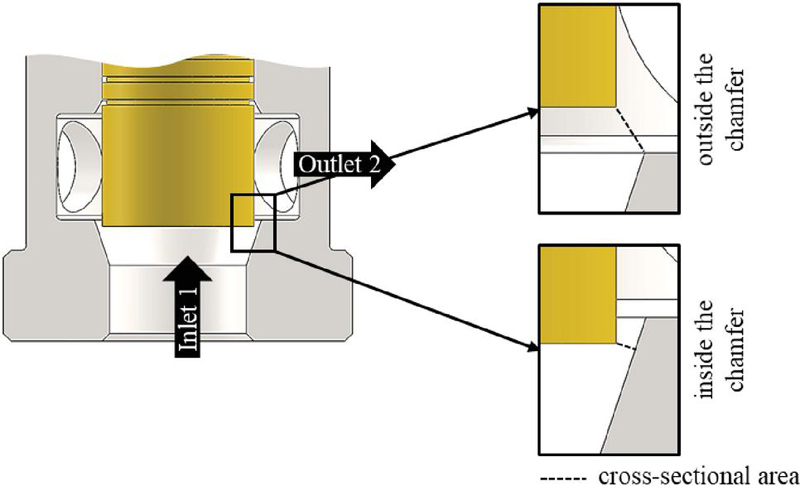
Figure 2 Conventional cartridge valve, exemplary flow direction $1\to 2$ through the assembly (left), definition of the cross-sectional area, outside the chamfer (top right), inside the chamfer (bottom right).

2 Methodology

The flow force calculation can be done in different ways. A simple and in most cases effective method is the determination of the resulting force using the conservation of momentum. Another advantage is that the dependencies can be easily identified through such an analytical relationship. For a defined control volume $\mathrm{\Omega }$, time-dependent (I), incoming and outgoing (II) momentum, as well as pressure forces (III) and shear forces (IV) or volume-dependent forces, such as acceleration forces (V), and body forces (VI) can be taken into account via the boundary S. As shown in Equation (2), the complete relation of the conservation of momentum is described in integral form.

$\underset{\mathrm{I}}{\underbrace{{\displaystyle {\int }_{\mathrm{\Omega }}}{\displaystyle \frac{\partial \rho \overrightarrow{\mathrm{u}}}{\partial \mathrm{t}}}\mathrm{dV}}}+\underset{\mathrm{II}}{\underbrace{{\displaystyle {\int }_{\mathrm{S}}}\rho \overrightarrow{\mathrm{u}}(\overrightarrow{\mathrm{u}}\cdot \overrightarrow{\mathrm{n}})\mathrm{dS}}}$

$\mathrm{\hspace{1em}}=\underset{\mathrm{III}}{\underbrace{-{\displaystyle {\int }_{\mathrm{S}}}\mathrm{p}\overrightarrow{\mathrm{n}}\mathrm{dS}}}+\underset{\mathrm{IV}}{\underbrace{{\displaystyle {\int }_{\mathrm{S}}}\overline{\overline{\tau }}\cdot \overrightarrow{\mathrm{n}}\mathrm{dS}}}+\underset{\mathrm{V}}{\underbrace{{\displaystyle {\int }_{\mathrm{\Omega }}}\rho \overrightarrow{\mathrm{f}}\mathrm{dV}}}+\underset{\mathrm{VI}}{\underbrace{{\overrightarrow{\mathrm{F}}}_{\mathrm{B}}}}$

(1)

For the hydraulic application regarding to valves, the following simplification can be assumed, which reduces the expression, Figure 3.

Steady state:	${\displaystyle \frac{\partial }{\partial \mathrm{t}}}=0$
Pressure compensated*:	${\displaystyle {\int }_{\mathrm{S}}}\mathrm{p}\overrightarrow{\mathrm{n}}\mathrm{dS}=0$
Flows close to the wall are very small compared to the resulting body forces (${\overrightarrow{\mathrm{F}}}_{\overline{\overline{\tau }}}\ll {\overrightarrow{\mathrm{F}}}_{\mathrm{B}}$) [11]:	${\displaystyle {\int }_{\mathrm{S}}}\overline{\overline{\tau }}\cdot \overrightarrow{\mathrm{n}}\mathrm{dS}=0$
Movement of the volume is neglected:	${\displaystyle {\int }_{\mathrm{\Omega }}}\rho \overrightarrow{\mathrm{f}}\mathrm{dV}=0$
*…The simplification of the pressure compensation assumes there are no impact zones on walls of the control volume caused by free jets. Because of too many influencing effects to the behaviour of the flow in such complex geometries it is difficult to describe this anomaly of the wall pressure. That means the calculated momentum is limited only to the dynamic part caused by flows over the inlet and outlet.

Figure 3 Application of the law of conservation of momentum on the basis of the rotary slide valve, valve spool (yellow), housing (light gray), control volume $\mathrm{\Omega }$ (black, dashed).

This results in an equation that describes only the dynamic part of the flow. The momentum entering and leaving the control volume determine it.

$${\int }_{\check{\mathrm{S}}}\rho \overrightarrow{\mathrm{u}}(\overrightarrow{\mathrm{u}}\cdot \overrightarrow{\mathrm{n}})\mathrm{dS}={\overrightarrow{\mathrm{F}}}_{\mathrm{B}}$$

(2)

Equation (2) can be explained as the tangential force part of the momentum, Equation (3). With the cylindrical coordinates it becomes easier to apply to the control volume of the rotary slide valve. The momentum of the outlet is perpendicular to the flow over the control edge. Thus there is no influence in the equations.

$${\mathrm{F}}_{\mathrm{flow}}=-\rho |{\overrightarrow{\mathrm{u}}}_{\mathrm{in}}^2|\cdot {\mathrm{A}}_{\mathrm{in}}\cdot \cos ({\epsilon }_{\mathrm{avg}})$$	(3)
$${\mathrm{T}}_{\mathrm{R}}=\int {\mathrm{F}}_{\mathrm{flow}}\mathrm{dr}=-\rho |{\overrightarrow{\mathrm{u}}}_{\mathrm{in}}^2|\cdot {\mathrm{A}}_{\mathrm{in}}\cdot \mathrm{r}\cos ({\epsilon }_{\mathrm{avg}})$$	(4)

Equation (3) defines the flow force and (4) the resistance torque acting tangential on the valve spool per control edge. This type of flow force only acts at flows over inlet and outlet of the control volume. As already mentioned, it is easy to see that the flow force ${\mathrm{F}}_{\mathrm{flow}}$ as well as the resistance torque ${\mathrm{T}}_{\mathrm{R}}$ depend on the geometric parameters of the flow area ${\mathrm{A}}_{\mathrm{in}}$ and the averaged flow angle ${\epsilon }_{\mathrm{avg}}$. Since the area cannot be used as an influencing parameter in this case because it must necessarily be opened to release the flow cross section. Only the flow angle remains to actively influence the resistance torque of the flow at the control edge/ narrow section.

But how does the flow angle behave and how can it be influenced? In the following, the methodology for investigating and derivation will be explained.

Due to the lack of knowledge about the exact behaviour of the flow angle, the correlation is examined in a generic minimal model by using CFD. The geometry is selected in such a way that no disturbance effects can influence the flow. The focus is purely on the variation of the flow angle. It is shown in [1], that the flow angle has a significant dependency of the inlet geometry.

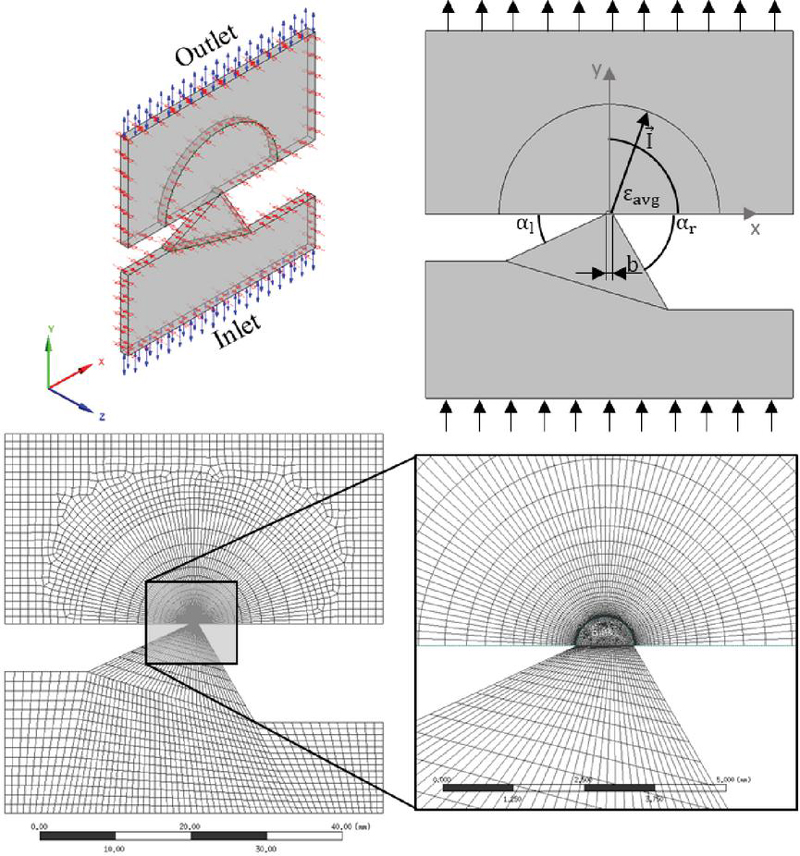
Figure 4 Overview of geometry of the model (top) and representation of meshing (overview – bottom left, bottleneck – bottom right)..

Figure 4 illustrates the flow simulation model, which is used to study the flow angle. The geometry is divided into inflow area (lower region), narrow section (center) and outflow area (upper region). The inlet region is variable using the angles ${\alpha }_{\mathrm{l}}$ and ${\alpha }_{\mathrm{r}}$ of the left and right walls. Thus, the flow angle of the free jet in the narrow section can be changed. The narrow section has a fixed width b of 1 mm and is arranged horizontally. The outlet region spans a free space starting from the narrow section in which the jet can spread freely. Due to many symmetrical relationships in technical geometries, a two-dimensional model is used for this investigation. The setup of the simulation model is summarized in Table 1. With the aid of this model, a new analytical method will be established to determine the flow angle at a narrow section very well (ch. 3.3, Equation (13)). The correlation shows a simplified expression between the inlet geometry and the flow angle of the free jet. The comparison of a real application is made in ch. 4.

Table 1 Minimal model – setup

Property	Setting	Property	Setting
geometrical variation		analysis type
${\alpha }_{\mathrm{l}}$	${\{0\mathrm{\dots }180\}}^{\circ }$	temporal consideration	steady state
${\alpha }_{\mathrm{r}}$	${\{0\mathrm{\dots }180\}}^{\circ }$	turbulence	Shear Stress Transport model (RANS)
$\mathrm{b}$	$1\mathrm{mm}$	convergence
boundary conditions		convergence criterion	${10}^{-4}$
inlet	opening with ${\mathrm{p}}_{\mathrm{in}}=\{{10}^{-4}\mathrm{\dots }{10}^2\}\mathrm{bar}$	max. number of time steps	200
outlet	opening with ${\mathrm{p}}_{\mathrm{out}}=0\mathrm{bar}$	fluid properties
wall	no slip wall (geometry related to x-y-plane)	density	863 kg/m${}^3$, incompressible
symmetry	in z-direction	kin. viscosity	46 mm${}^2$/s
		temperature	40${}^{\circ }$C, isotherm

3 Flow angle of free jets on the minimal model

This chapter deals with the study of the properties and derivation of the flow angle. For a better understanding, the following structure is used.

• general definition of the local and averaged flow angle

• laminar and turbulent influence

• analytical method for the averaged flow angle

3.1 Definition of the Flow Angle $\mathit{\epsilon }$

The local flow angle ${\epsilon }_{\mathrm{loc}}$ at a given point in the fluid domain is defined by the velocity components u (x-direction) and v (y-direction), see Equation (5). To determine the averaged flow angle ${\epsilon }_{\mathrm{avg}}$, the flow angle ${\epsilon }_{\mathrm{loc}}$ is averaged over the width b at the narrow section, as shown in Equation (6). For the investigation, the flow angle is calculated at $\mathrm{y}={\mathrm{y}}_0=0$, the position of the narrow section.

$${\epsilon }_{\mathrm{loc}}=\mathrm{atan}\left(\frac{\mathrm{v}}{\mathrm{u}}\right)$$	(5)
$${\epsilon }_{\mathrm{avg}}=\frac{1}{\mathrm{b}}{\int }_{-\mathrm{b}/2}^{\mathrm{b}/2}{\epsilon }_{\mathrm{loc}}({\mathrm{y}}_0,\mathrm{x})\mathrm{dx}$$	(6)

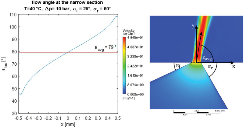
Figure 5 Flow angle ${\epsilon }_{\mathrm{loc}}$ at the narrow section for the case: ${\alpha }_{\mathrm{l}}={25}^{\circ }$, ${\alpha }_{\mathrm{r}}={60}^{\circ }$, $\mathrm{\Delta }\mathrm{p}=10\mathrm{bar}$, flow angle plotted over the opening coordinate x (left), velocity field of the free jet around the narrow section (right).

In Figure 5, the flow angle ${\epsilon }_{\mathrm{loc}}$ in the narrow section over the opening coordinate x is shown. The left diagram clarifies the profile of the flow angle between the left and right edges of the narrow section. Due to the Neumann (no slip) boundary conditions along a wall, the flow angle at the edges is equal or very similar to the orientation of the wall. On the left wall the geometrical angle ${\alpha }_{\mathrm{l}}$ is 25${}^{\circ }$ and the the flow angle is about 45${}^{\circ }$. On the right side the geometrical angle ${\alpha }_{\mathrm{r}}$ is ${60}^{\circ }$ and the flow angle is about 108${}^{\circ }$ (related to ${\alpha }_{\mathrm{r}}$ 72${}^{\circ }$). The deviations are caused by a strong rotation of the flow in the corners of the narrow section. The averaged value of the angle is ${\epsilon }_{\mathrm{avg}}={79}^{\circ }$.

3.2 Laminar and Turbulent Influence

In this section the range of validity of the calculation of the averaged flow angle ${\epsilon }_{\mathrm{avg}}$ for different Reynolds numbers is investigated. Decisive here is the consideration of a laminar and/or turbulent flow. According to [12] with reference to [13], the critical Reynolds number of a free jet is $\mathrm{Re}\approx 30$. The Reynolds number is defined here as follows.

$$\mathrm{Re}=\frac{\tilde{\mathrm{u}}\cdot \mathrm{l}}{\nu }\mathit{\hspace{1em}}\mathrm{with}\nu =\frac{\eta }{\rho }$$

(7)

The velocity $\tilde{\mathrm{u}}$ is defined such as the characteristic length $\mathrm{l}=\mathrm{b}$ at the narrow section of the free jet. The Equation (7) is illustrated by following example. A valve of nominal size 08 according to ISO 7368 is opened to 20% and operates with a volume flow of 15 l/min. According to [14], this area of the valve is strongly in the laminar region of hydraulic resistance. The calculated Reynolds number Re $=$ 138 is well above the critical value of 30. That means the flow is nevertheless predominantly laminar in the gap per se. Due to the superposition of laminar and turbulent flow, the resulting free jet behind the narrow section is nevertheless turbulent. It is clear there is a strictly separation between the laminar and turbulent behaviour of a hydraulic resistance and the characteristics of a free jet.

In the following, it will be shown that a turbulent free jet is almost always present for hydraulic components. This also applies to the minimal model. With the fluid properties of HLP 46 (Table 1), the following course of the Reynolds number over the pressure drop is obtained for the geometry, see Figure 6. In the diagram on the left, the Reynolds number is plotted against the pressure drop $\mathrm{\Delta }\mathrm{p}$. It includes the marked operating points investigated for this study. In order to gain a better understanding of the influence of temperature on the Reynolds number and thus on turbulence, the characteristic curve for 20${}^{\circ }$C and 100${}^{\circ }$C is shown in addition to the 40${}^{\circ }$C curve. It shows that an undercutting of the limiting $\mathrm{Re}\approx 30$ (red line) is given even at lower temperatures like 20${}^{\circ }$C for pressure drops smaller than 1 bar. A classical hydraulic application has much higher operating points. It shows that a laminar flow is only important in special cases of very low pressure drops and over large narrow sections. However, in such special cases effects like flow forces are negligible compared to static pressure forces. The reason for these cases with very low velocities is the quadratic contribution of the flow force, see Equation (3).

Figure 6 Investigation of the laminar-turbulent influence for the case: “${\alpha }_{\mathrm{l}}={25}^{\circ }$, ${\alpha }_{\mathrm{r}}={60}^{\circ }$” Reynolds number plotted over pressure drop for various temperatures (left), velocity fields of the free jet for Reynolds numbers at (a’) to (d’).

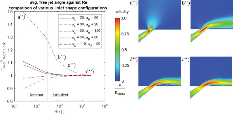
Figure 7 Averaged flow angle ${\epsilon }_{\mathrm{avg}}$ against the Reynolds number for various geometrical inlet shape configurations (${\alpha }_{\mathrm{l}}$, ${\alpha }_{\mathrm{r}}$, left), the influence on acute and flat boundary cases (right).

On the right side in Figure 6, the velocity fields for the operating points a’) to d’) are shown for the geometrical inlet shape configuration from Figure 5 (${\alpha }_{\mathrm{l}}={25}^{\circ }$, ${\alpha }_{\mathrm{r}}={60}^{\circ }$). It can be seen how the shape of the free jet is influenced by increasing Reynolds number. For $\mathrm{Re}>30$ the shape of the free jet is fully developed and has a sharp separation between the free jet velocity field and the static environment. For $\mathrm{Re}<30$ the shear layer has almost disappeared and it prevails a laminar flow.

The correlation between the averaged flow angle ${\epsilon }_{\mathrm{avg}}$ against the Reynolds number for various geometrical inlet shape configurations (${\alpha }_{\mathrm{l}}$, ${\alpha }_{\mathrm{r}}$) will be discussed in Figure 7. The left diagram illustrates the normalized averaged flow angle ${\epsilon }_{\mathrm{avg}}/{\epsilon }_{\mathrm{avg100bar}}$ (normalized to turbulent flow) against the Reynolds number. A deviation is recognizable between the turbulent and the laminar flow for all cases. With exception of the case “${\alpha }_{\mathrm{l}}={30}^{\circ }$, ${\alpha }_{\mathrm{r}}={140}^{\circ }$” for $\mathrm{Re}>30$ all averaged flow angles stay almost the same and converge. Only for $\mathrm{Re}<30$ it deviates up to 10% of the reference value. The reason for that is the influence of the laminar flow. The special case “${\alpha }_{\mathrm{l}}={30}^{\circ },{\alpha }_{\mathrm{r}}={140}^{\circ }$” already shows a much higher deviation at larger Reynolds numbers. For better understanding, the right side of the figure shows the configuration for cases a”) to d”) by increasing Reynolds numbers. Due the very flat inlet the free jet is attached to the wall even if the flows is turbulent. This effect is called Coanda effect, [12] and [15]. For certain inclinations of the free jet to the wall the suction area of the free jet leads to the fact that the free jet is aligned with the wall, [14] and [15]. For inlet shape configurations in this range, larger deviations are to be expected.

In summary, most important for hydraulic applications is the turbulent free jet. In contrast to the hydraulic resistance description the laminar and turbulent behavior of a flow is always considered in parallel as principle of superposition, as shown in [1]. The current investigation focuses on the free jet angle. The flow resistance of hydraulic components is not taken into account. Thus, it must not be confused with the laminar free jet at this point.

Because of its predominantly turbulent behavior, all further considerations are performed for the turbulent free jet.

3.3 Analytical Method for the Averaged Flow Angle

The derivation of the averaged flow angle ${\epsilon }_{\mathrm{avg}}$ for a turbulent free jet is illustrated in Figure 8. In a) it can be seen an overview of the geometry near the narrow section including the inlet and outlet momentum. The momentum in the inlet is aligned according to the flow angle. The range of the flow angle is limited through geometrical parameters ${\alpha }_{\mathrm{l}}$ and ${\alpha }_{\mathrm{r}}$. The right side (b) shows the course of the flow angle along the narrow section (see Figure 5). Regarding to ch. 3.1 the averaged flow angle lies in the center point of the narrow section. Additionally the course of $\epsilon (\mathrm{x})$ can be separated in two parts. The first one $\epsilon {(\mathrm{x})}^{*}$ is a point symmetrical graph with its center point in the coordinate origin. The second part is a constant offset ${\epsilon }_{\mathrm{avg}}$. In summary the equation for $\epsilon (\mathrm{x})$ is:

$$\epsilon (\mathrm{x})=\epsilon {(\mathrm{x})}^{*}+{\epsilon }_{\mathrm{avg}}$$

(8)

It is necessary to set an unproven but plausible assumption to make a reference to the momentum. The absolute value of the momentum over the flow angle in the inlet is uniform. Thus, the momentum can be written as $\overrightarrow{\mathrm{I}}(\epsilon )=\overrightarrow{\mathrm{e}}(\epsilon )|\overrightarrow{\mathrm{I}}|$. In this formula $\overrightarrow{\mathrm{e}}(\epsilon )$ is the unit vector with the direction of $\epsilon$. That means the whole fluid in the inlet moves uniformly towards to the narrow section.

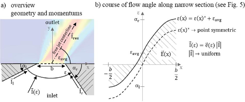
Figure 8 Prediction of the averaged flow angle ${\epsilon }_{\mathrm{avg}}$ – simplified model to consider the incoming and outgoing momentum (a), course of the flow angle along the narrow section (b).

In the following, the relationship between the averaged flow angle and the geometry is derived from the assumptions just mentioned. Regarding to Equation (6) the first mean value theorem is applied to the whole course of $\epsilon$ according to Figure 8b). Integrating over the graph of $\epsilon (\mathrm{x})$ yields the following expression.

$${\epsilon }_{\mathrm{avg}}=\frac{1}{\mathrm{b}}{\int }_{-\mathrm{b}/2}^{\mathrm{b}/2}\epsilon (\mathrm{x})\mathrm{dx}=\frac{1}{\mathrm{b}}[\mathrm{E}(\mathrm{b}/2)-\mathrm{E}(-\mathrm{b}/2)]$$

(9)

In this case $\mathrm{E}$ is the root function of $\epsilon$. With the possibility to separate $\epsilon \left(\mathrm{x}\right)$ such as in Equation (8), Equation (9) can be extended and rearranged.

$${\epsilon }_{\mathrm{avg}}=\frac{1}{2}\left[\left(\frac{\mathrm{E}{(\mathrm{b}/2)}^{*}}{\mathrm{b}/2}+{\epsilon }_{\mathrm{avg}}\right)-\left(\frac{\mathrm{E}{(-\mathrm{b}/2)}^{*}}{\mathrm{b}/2}-{\epsilon }_{\mathrm{avg}}\right)\right]$$

(10)

The expression ${(\cdot )}^{*}$ symbolizes the point symmetrical part of the course. The separation remains in the root functions. The first term $\frac{\mathrm{E}{(\pm \mathrm{b}/2)}^{*}}{\mathrm{b}/2}$ describes the mean increase of the function for the respective interval [0, $\mathrm{b}/2$] (case 1, left term) and [$-\mathrm{b}/2$, 0] (case 2, right term). The second part is only the offset. Both formula have the same structure like Equation (8). By means of case separation between the two intervals case 1 and case 2, Equation (8) can be integrated into Equation (10).

In case 1 with the interval [0, $\mathrm{b}/2$], a linear equation is set up, which is to be determined at x $=$ b/2. The increase of the function is defined over the whole interval with $\mathrm{\Delta }\mathrm{E}/\mathrm{\Delta }\mathrm{x}$. The offset is clarified through ${\epsilon }_{\mathrm{avg}}$. Case 2 can be described analogously. Equation (11) shows for both intervals the expression in the form of Equation (8).

$\tilde{\epsilon }(\mathrm{b}/2)$	$={\displaystyle \frac{\mathrm{E}{(\mathrm{b}/2)}^{*}-\mathrm{E}(0)}{\mathrm{b}/2}}+{\epsilon }_{\mathrm{avg}}$
	$=\mathrm{k}\epsilon {(\mathrm{b}/2)}^{*}+{\epsilon }_{\mathrm{avg}}\mathit{\hspace{1em}}\mathrm{for}[0,\mathrm{b}/2]$
$-\tilde{\epsilon }(-\mathrm{b}/2)$	$={\displaystyle \frac{\mathrm{E}(0)-\mathrm{E}{(-\mathrm{b}/2)}^{*}}{\mathrm{b}/2}}-{\epsilon }_{\mathrm{avg}}$
	$=-\mathrm{k}\epsilon {(-\mathrm{b}/2)}^{*}-{\epsilon }_{\mathrm{avg}}\mathit{\hspace{1em}}\mathrm{for}[-\mathrm{b}/2,0]$	(11)

The additional factor k is a scaling of the point symmetrical part of $\tilde{\epsilon }$ for integrating of Equation (8). With Equation (11) it is possible to extend Equation (10) to the following expression.

$${\epsilon }_{\mathrm{avg}}=\frac{1}{2}[\tilde{\epsilon }(\mathrm{b}/2)+\tilde{\epsilon }(-\mathrm{b}/2)]$$

(12)

Because of the point symmetrical characteristic of $\tilde{\epsilon }(\mathrm{x})$ as well as $\epsilon (\mathrm{x})$ the term $\epsilon {(\mathrm{x})}^{*}$ will always eliminate itself. The offset ${\epsilon }_{\mathrm{avg}}$ remains and the Equation (12) is fulfilled. Thus, Equation (12) is universal for all point symmetrical equations with a uniform offset.

That means for calculations of the flow angle at the narrow section, only the flow angle at the limiting walls must be known. Regarding to Figure 5 and the Neumann boundary conditions along a wall the flow angle and the local geometrical angle can be equated. It applies: $\tilde{\epsilon }(\mathrm{b}/2)=\pi -{\alpha }_{\mathrm{r}}$ and $\tilde{\epsilon }(-\mathrm{b}/2)={\alpha }_{\mathrm{l}}$. For a better illustration, Equation (12) can be extended to a vector sum of the inlet momentum with the reference to the resulting momentum of the free jet. The assumption $\overrightarrow{\mathrm{I}}(\epsilon )=\overrightarrow{\mathrm{e}}(\epsilon )|\overrightarrow{\mathrm{I}}|$ with $|\overrightarrow{\mathrm{I}}|$ as uniform is applied over the inlet area. The Figure 9 shows the relationship between the momentum of inlet and outlet.

Figure 9 Momentum of inlet (${\overrightarrow{\mathrm{I}}}_{\mathrm{l}}$ and ${\overrightarrow{\mathrm{I}}}_{\mathrm{r}}$) in reference to the outlet momentum ${\overrightarrow{\mathrm{I}}}_{\mathrm{res}}$.

For the calculation, the relationship is transferred into Cartesian coordinates. With the expression ${\overrightarrow{\mathrm{I}}}_{{\mathrm{i}}_{\mathrm{x}}}({\alpha }_{\mathrm{i}})={\overrightarrow{\mathrm{I}}}_{\mathrm{i}}\cos ({\alpha }_{\mathrm{i}})$ all angle dependent momentum can be related to the x component. The Figure 9 illustrates sum of the x components aligned to the abscissa. According to this principle, Equation (12) can be transferred into the x component of the Cartesian coordinates, as shown in Equation (13).

$$\mathit{c}\mathit{o}\mathit{s}({\mathit{\epsilon }}_{\mathit{a}\mathit{v}\mathit{g}})=\frac{\mathbf{1}}{\mathbf{2}}(\mathit{c}\mathit{o}\mathit{s}({\mathit{\alpha }}_{\mathit{l}})-\mathit{c}\mathit{o}\mathit{s}({\mathit{\alpha }}_{\mathit{r}}))$$

(13)

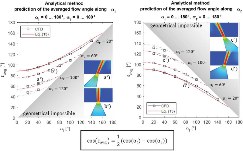
Figure 10 Prediction of the averaged flow angle ${\epsilon }_{\mathrm{avg}}$ – comparison between Equation (13) and CFD data, plotted over ${\alpha }_{\mathrm{l}}={\{0\mathrm{\dots }180\}}^{\circ }$ (left) and ${\alpha }_{\mathrm{r}}={\{0\mathrm{\dots }180\}}^{\circ }$ (right).

Equation (13) is the major finding of this work. It describes the correlation between the geometrical angles ${\alpha }_{\mathrm{L}},{\alpha }_{\mathrm{r}}$ and the averaged flow angle ${\epsilon }_{\mathrm{avg}}$. This equation allows the direct calculation of the flow angle from the geometry of the narrow section only. It is independent of any operating conditions (see ch. 3.2). As an example, Equation (13) gives a flow angle of 78,3${}^{\circ }$ when the geometrical data from Figure 5 are used. This matches very well with the CFD results of 79${}^{\circ }$.

Figure 10 shows the comparison of the Equation (13) and the CFD data over the full range of ${\alpha }_{\mathrm{l}}$ and ${\alpha }_{\mathrm{r}}$. Geometrical impossible configurations, when ${\alpha }_{\mathrm{l}}+{\alpha }_{\mathrm{r}}>{180}^{\circ }$, are colored grey in the diagram. It can be seen that for all geometric shapes, the values calculated by Equation (13) match very well with the CFD results. Only for the limiting cases ${\alpha }_{\mathrm{l}}\gg {\alpha }_{\mathrm{r}}$ as well as ${\alpha }_{\mathrm{l}}\ll {\alpha }_{\mathrm{r}}$ a slight deviation is observed. The deviations are smaller than 10% for the special cases and thus acceptable. In another cases ${\alpha }_{\mathrm{l}}=0^{\circ }$ and ${\alpha }_{\mathrm{r}}=0^{\circ }$, the free jet angle can only vary between 0${}^{\circ }$ and 90${}^{\circ }$ or from 90${}^{\circ }$ to 180${}^{\circ }$. If both inlet angles are identical, the free jet angle is always constant 90${}^{\circ }$, as shown in the velocity field of configuration b’). This special case enables a symmetrical flow through the inlet geometry and generates a “classic” vertical free jet.

In summary, the Equation (13) shows very good results compared to the minimal model. The simple expression represents a connection to geometrical parameters only and is not related to any operation conditions. The assumptions for this derivation is valid for turbulent flow. Thus, it is useable for almost all applications of hydraulic systems.

4 Transfer to Real Application

In this chapter Equation (13) is applied to two valve concepts – a rotary slide valve and a conventional cartridge valve. The first application is about the flow angle calculation in the rotary slide valve. The focus lies on the evaluation of the transferability to real application. Thus the flow angle is compared with CFD data for different inlet geometry configurations. With the modification of the flow angle the resistance torque can be improved by 65%.

Figure 11 Rotary slide valve, geometrical setup (a), comparison between CFD data and the Equation (13) along ${\alpha }_{\mathrm{in}}={\{0\mathrm{\dots }75\}}^{\circ }$ for different twisting angles $\phi ={\{10,20,30\}}^{\circ }$ (b), velocity field in symmetrical plane through the narrow sections for different configuration of ${\alpha }_{\mathrm{in}}=\{0^{\circ },{45}^{\circ }\}$, ${\mathrm{Q}}_{\mathrm{n}}=40\mathrm{l}/\min$, flow direction $1\to 2$ (see Figure 1).

In the second application Equation (13) is integrated into Equation (3) to predict the flow force of the cartridge valve. The correlation between Equation (13) and the CFD data is very good for control edges outside of the chamfer. It is also shown where the limits of the definition of the flow angle lie.

4.1 Rotary Slide Valve

Prediction of the flow angle

In the following, the Equation (13) is evaluated by using the rotary slide valve. Figure 11 shows the comparison between CFD data with the results of Equation (13). In a) the geometrical characteristics of the narrow section is defined. The influencing angle in the inlet of the valve is ${\alpha }_{\mathrm{in}}$. The angle ${\alpha }_{\mathrm{in}}$ is valid in the range between 0${}^{\circ }$ (vertical inlet) to 75${}^{\circ }$. The relationship between ${\alpha }_{\mathrm{in}}$ and the angles ${\alpha }_{\mathrm{l}}$ and ${\alpha }_{\mathrm{r}}$ of Equation (13) is illustrated in figure a). The setup of all simulations is similar to Table 1 and is expected to the parameter variation with ${\alpha }_{\mathrm{in}}$. In b) the absolute values of the averaged flow angle as well as the relative deviation between CFD data and Equation (13) are plotted over ${\alpha }_{\mathrm{in}}$ for different twisting angles $\phi$. The angle ${\alpha }_{\mathrm{r}}$ corresponds to the inverse behavior of the angle ${\alpha }_{\mathrm{in}}$ (${\alpha }_{\mathrm{r}}={90}^{\circ }-{\alpha }_{\mathrm{in}})$. Additionally, ${\alpha }_{\mathrm{l}}$ have a variation from 0${}^{\circ }$ (almost closed) to $-$15${}^{\circ }$ (almost fully open) dependent on the twisting angle. The reason for that is the convex shape of the outer surface of the valve spool. In order of the Equation (13) to be applied, the geometric conditions must be established from Figure 8. Regarding to Figure 10 right side, the graph of the absolute values shows a very similar course. For ${\alpha }_{\mathrm{in}}>{20}^{\circ }$ the results between CFD and Equation (13) match very well and the relative deviation is below 5%. It proves that the explained calculation method is reliable. In the range of ${\alpha }_{\mathrm{in}}<{20}^{\circ }$ the scattering of the values becomes larger between different twisting angles and the relative deviation is the highest in this course with about $+$10%. However, for an engineering application the deviations are still acceptable. The results in general are in line with the statement from Figure 10.

For a better understanding how the fluid domain is modified, in a’) and b’) the velocity field in a symmetrical plane through the narrow sections is shown for different configurations of ${\alpha }_{\mathrm{in}}=\{0^{\circ },{45}^{\circ }\}$. The plot a’) shows the default configuration with a vertical inlet. The free jets flow much more flatly into the geometry and have large contact regions with the wall. The second one, b’), clarifies the modified inlet shape. The free jets meet in the center and partially dissipate themselves. Thus, the resistance torque can be significantly reduced (next paragraph). It is recognizable how ${\alpha }_{\mathrm{in}}$ influence the flow angle of the free jet.

To sum up, the new method of Equation (13) allows a reliable prediction of the flow angle of free jets. Same results can be achieved for complex geometries as the rotary slide valve. It is possible to influence actively the jet direction after the narrow section. Looking at other issues such as cavitation collapse regions (erosion regions) or stagnation points in general, the potential for improvement using Equation (13) is high.

Improvement of the rotary slide valve

The main goal of the improvement of the valve is the reduction of the resistance torque which is strongly dependent on the flow force. As shown in Equation (3) the flow force is mainly influenced by the flow angle at the narrow section. With the results of the previous paragraph, the following improvements could be made by CFD, as shown in Figure 12. The characteristic curves for pressure drop (a) and the resistance torque (b) over $\phi$ are plotted for the default (black) and the modified (red) valve design and both flow directions (see Figure 1). The direction $1\to 2$ is marked as solid line and $2\to 1$ as dashed line. In addition, both characteristic curves are simulated by a constant nominal flow rate ${\mathrm{Q}}_{\mathrm{n}}$. Comparing to pressure drop across $\phi$ (a), the results for both designs are similar. Moreover, the gradient is almost identical. There is only an angular offset of $1^{\circ }$ to $2^{\circ }$. Significant changes can be seen in the resistance torque. Especially for the flow of $1\to 2$, the amount in the maximum range decreases by 65% from 0.23 Nm to 0.08 Nm. The resistance torque of $2\to 1$, on the other hand, is negatively affected. However, this effect is significantly smaller and can be accepted at this point. In order to actively influence the flow direction $2\to 1$, the inlet angle of the inner geometry of the rotary slide valve would have to be varied according to this principle. Unfortunately, cost-related changes are not acceptable for cost optimized part usage in industrial applications.

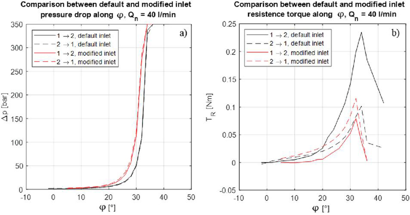
Figure 12 Improvement of the modification, comparison of the pressure drop across $\phi$ at constant flow rate (a) and of the resistance torque across $\phi$ (c), in each case for both flow directions, ${\mathrm{Q}}_{\mathrm{n}}=40\mathrm{l}/\min$.

Because of the preferred horizontal inlet flow into the control volume of the valve the calculation of the resistance torque by Equation (4) is not useful. Hence, the results were generated by CFD. Various impact zones of the free jets along the wall of the control volume, as shown in Figure 11 a’) and b’), need an additional expression for the wall pressure. As already mentioned, the calculated momentum is limited only to the dynamic part caused by flows over the inlet and outlet.

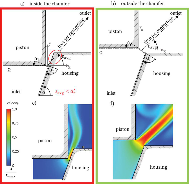
Figure 13 Cartridge valve, schematic illustration of the various positions of the piston with all parameters to apply Equation (13), piston inside the chamfer (left side, Equation (13) invalid) and piston outside the chamfer (right side, Equation (13) valid).

In summary, the flow force improvement by using flow angle modification according to Equation (13) is very effective. The main setup of the geometry is unchanged and only the inlet shape near the narrow section has to be modified. The impacts of this modification are enormous and the production effort is kept within limits.

4.2 Cartridge Valve

Definition of the flow angle

As already mentioned, the used cartridge valve has two different definitions of the control edge, as shown in Figure 2. The Figure 13 is the simplified geometry to apply Equation (13) and illustrates these two positions of the piston more detailed. The narrow section inside the chamfer is on the left and outside the chamfer on the right. Additionally, the geometry parameter ${\alpha }_{\mathrm{l}}$ and ${\alpha }_{\mathrm{r}}$, the averaged flow angle ${\epsilon }_{\mathrm{avg}}$ as well as the control volume $\mathrm{\Omega }$ at the bottom of the piston are defined. Decisive for the definition of the flow angle and later for the flow force is the position of the inlet and outlet boundary of the control volume. In that case the outlet boundary at the narrow section is important. The fluid flows over the boundary of the control volume and generates the dynamic part of the flow force. On the left side of Figure 13 with a red frame the narrow section is defined at the bottom edge of the piston and is perpendicular to the chamfer. Behind the narrow section the chamfer continues. This geometric restriction downstream influenced the direction of the free jet. The calculated flow angle at the narrow section is smaller than the geometry angle of the chamfer (see Figure 13a). That means the free jet is transformed into a wall jet and Equation (13) is no longer valid. The following example illustrates the effect. It can be assumed the geometry parameter ${\alpha }_{\mathrm{r}}^{\prime }={70}^{\circ }$. With the geometry definition of Figure 13, left side, and Equation (13) ${\epsilon }_{\mathrm{avg}}$ can be calculated. For that case the flow angle ${\epsilon }_{\mathrm{avg}}\approx {42}^{\circ }$ is significant lower than the restrictive angle ${\alpha }_{\mathrm{r}}^{\prime }$. The consequence of this is a wall jet along the chamfer with other characteristics such as a free jet. On the right side of Figure 13 with a green frame the piston is outside the chamfer. Equation (13) is correctly defined as in Figure 8. Hence, for the following flow force prediction is only valid for strokes, where the piston is outside the chamfer.

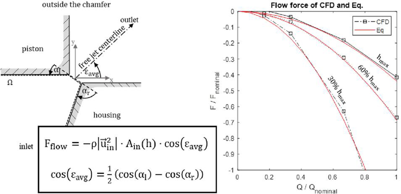
Figure 14 Cartridge valve, schematic illustration of the valid piston configuration with the important equations (Equations (3) and (13)) (left side) and the results of the flow force calculation compared with CFD data.

To sum up, it is important to clarify the geometry definition if Equation (13) is to be used. In that case a simple plausibility analysis is sufficient to prove validity. In general the Equation (13) is valid for geometries similar to Figure 8. If there is a constricted geometry downstream of the narrow section the flow angle is influenced and Equation (13) cannot be applied.

Prediction of the flow force

To predict the flow force analytically Equation (3) has to be combined with Equation (13). This approach is only valid for geometries with no restrictions downstream of the narrow section. Hence, only the right side of Figure 13 is able to be calculated. To sum up the configuration Figure 14 on the left illustrates the geometry and the two important equation (Equation (3) and Equation (13)). The results are shown in Figure 14 on the right and are compared with CFD data. The CFD data represents the geometry of Figure 2. Thus, the analytical approach with a simplified geometry (see Figure 13) is contrasted to the CFD with the realistic geometry. The flow force is plotted over the volume flow for specific strokes. All values are normalized by the nominal values of the valve characteristic. The analytical approach and the CFD data match very well. The courses show the typical quadratic progression that results from the volume flow. Additionally all values are negative. That means the direction of action of the flow force is closing the piston (regarding to the coordinate system in Figure 13b)).

It can be shown how well this approach works for sharp edges in a valve. Thus, the Equation (13) has only two limitations. The first one is the geometrical configuration. If there is a restriction downstream of the narrow section the forming jet flows along the wall. The typical behaviour of a free jet is no longer valid and the flow angle in the narrow section deviates from the calculated by Equation (13). Additionally, it is important to take the geometry of the piston into account. In this case (see Figure 2) the piston has one surface influenced by the flow (on the bottom). Thus the flow force is only related to this surface and the flow behind the narrow section has no major significance. The new approach can be applied. However, for two-stepped pistons there is a second ring-shaped surface in the outlet region. Then it is important to take the downstream region also into account. For such valve types with two surfaces influenced by the flow the approach is no longer sufficient. The geometry of the bushing wall and holes are quite near to the narrow section of the piston and significantly influence the downstream flow. The second limitation are very low Reynolds numbers ($\mathrm{Re}\approx 30$, see Figure 7). In this operation range the flow behaviour is more laminar than turbulent and Equation (13) is no longer valid.

5 Discussion and Conclusion

In summary, the following conclusions could be drawn with the help of the presented research.

Turbulent-laminar operating conditions

For turbulent flows, the averaged flow angle is independent of the operating point. In the range of laminar flows there is a clearly deviation compared to turbulent flow angles. Due to the low Reynolds number of $\mathrm{Re}\approx 30$, this effect is outside the operating conditions of “classical” hydraulic applications. Therefore, the operating range is always in the turbulent range and a behaviour independent of the operating point is to be expected.

Analytical method for the determination of the flow angle

The new method according to Equation (13), the averaged flow angle can be predicted with very good approximation. Slight deviations are only to be expected in ranges of ${\alpha }_{\mathrm{l}}\gg {\alpha }_{\mathrm{r}}$ as well as ${\alpha }_{\mathrm{l}}\ll {\alpha }_{\mathrm{r}}$, which can amount to a maximum deviation of 10%. The simple expression represents only a dependency to geometrical parameters and is not related to any operation conditions. The assumptions for this derivation is valid for turbulent flow. Thus, it is useable for almost all applications of hydraulic systems.

Transferability to real applications

The new method of Equation (13) allows a reliable prediction of the flow angle of free jets which is also applicable for a wide range of hydraulic geometries. It is possible to adjust the jet direction after the narrow section. Looking at other issues such as cavitation collapse regions (erosion regions) or stagnation points in general, the potential for improvement using Equation (13) is high. The main setup of the geometry is unchanged and only the inlet shape near the narrow section has to be modified. The impacts of this modification are enormous and the production effort is kept within limits.

Limitation of the approach

There are primarily two limitations for the usage of Equation (13). The first one is the geometrical configuration. The underlying phenomenon is the free jet at a sharp edge. Thus, a restrictions downstream of the narrow section cannot be represented by the Equation (13), as exemplary shown in Figure 13. For calculations of restrictions in the downstream section, it is advisable to use the method from [16]. Additionally, the surfaces influenced by the flow has to be taken into account. For single surface pistons such as Figure 2, the approach can be applied. For two-stepped pistons it is no longer sufficient. Another limitation are very low Reynolds numbers (Re $<$ 30). In this operation range the free jet is no longer turbulent and derivation of the flow angle increases.

Nomenclature

A	Area	m${}^2$
b	width	m
f	acceleration	m/s${}^2$
F	force	N
I	momentum	N s
l	characteristic length	m
n	normal vector	-
p	pressure	bar
r	radius	m
S	boundary of control volume	m${}^2$
t	time	s
T	temperature	${}^{\circ }$C
TR	resistance torque	N m
u	velocity as vector or as component in x-direction	m/s
v	velocity as component in y-direction	m/s
V	volume	m${}^3$
x	coordinate direction	m
y	coordinate direction	m
$\alpha$	geometrical angle	${}^{\circ }$
$\mathrm{\Delta }$	difference	-
$\epsilon$	flow angle	${}^{\circ }$
$E$	Root function of $\epsilon$
$\eta$	dynamic viscosity	Pa s
$\mathit{\rho }$	density	kg/m${}^3$
$\mathit{\tau }$	shear stress tensor	Pa
$\upsilon$	kinematic viscosity	mm${}^2$/s
$\mathit{\phi }$	twisting angle	${}^{\circ }$
$\mathbf{\Omega }$	control volume	m${}^3$

Acknowledgement

The author would like to thank the institutions Bundesministerium für Bildung und Forschung (BMBF) and Europäische Union – NextGenertionEU for funding the project “Erarbeitung funktionsintegrierter Schaltventile für Maschinen, Anlagen und Fahrzeuge zur Senkung des Energieverbrauchs (funkiS)” with the funding code 01LY2004B. Also the authors gratefully acknowledge the computing time made available to them on the high-performance computer at the NHR Center of TU Dresden. This center is jointly supported by the Federal Ministry of Education and Research and the state governments participating in the NHR (https://www.nhr-verein.de/unsere-partnerwww.nhr-verein.de/unsere-partner).

References

[1] N. Gebhardt, J. Weber (2020) Hydraulik – Fluid-Mechatronik. Grundlagen, Komponenten, Systeme, Messtechnik und virtuelles Engineering. Dresden, January 2020, Dresden, Germany, ISBN 3-662-60663-1 7th edition.

[2] S. Osterland, L. Günther, J. Weber (2022) Experiments and Computational Fluid Dynamics on Vapor and Gas Cavitation for Oil Hydraulics. In: Chemical Engineering and Technology Vol. 46, Issue 1, (2023), DOI: https://doi.org/10.1002/ceat.202200465.

[3] S. Osterland, L. Müller, J. Weber (2021) Influence of Air Dissolved on Hydraulic Oil on Cavitation Erosion, In: Int. J. Fluid Power 2021, DOI: https://doi.org/10.13052/ijfp1439-9776.2234.

[4] R. Ivantysyn, A. El Shorbagy, J. Weber (2018) Schlussbericht – Smart Pump – decentralized control for vessel engine. Dresden, 2018, Dresden, Germany.

[5] M. Dietze, et al. (1996) Messungen und Berechnungen der Innenströmung in hydraulischen Sitzventilen. Technische Hochschule Darmstadt, 1996, Darmstadt, Germany.

[6] M. Kipping, et al. (1997) Experimentelle Untersuchungen und numerische Berechnungen zur Innen strömung in Schieberventilen in der Ölhydraulik. Technische Hochschule Darmstadt, 1997, Darmstadt, Germany.

[7] C. Latour, et al. (1996) Strömungskraftkompensation in hydraulischen Sitzventilen. RWTH Aachen, December 1996, Aachen, Germany.

[8] M. Ristic, et al. (2000) Dreidimensionale Strömungsberechnungen zur Optimierung von Hydraulikventilen bezüglich der stationären Strömungskräfte. RWTH Aachen, 2000, Aachen, Germany.

[9] K. Wanne, et al. (1965) Messung und Untersuchung der axialen Kräfte an ölhydraulische Steuerschiebern. Technische Hochschule Stuttgart, 1965, Stuttgart, Germany.

[10] M. Lechtschewski, et al. (1994) Untersuchung der Abhängigkeit der Strömungskraft vom Hub des Ventilschiebers und der Druckdifferenz. Institut für Werkzeugmaschinen und Fluidtechnik, TU Dresden, 1994, Dresden, Germany.

[11] S. Osterland, J. Weber (2016) A numerical study of high pressure flow through a hydrsulic pressure relief valve considering pressure and temperature dependent viscosity, bulk modulus and density. In: 9th FPNI Ph.D. Symposium on Fluid Power, 2016 Florianópolis, Brazil. DOI: https://doi.org/10.1115/FPNI2016-1515.

[12] H. Schlichting, K. Gersten (1996) Grenzschicht-Theorie. Springer-Verlag, 1996, Bochum, Germany, ISBN: 3-540-55744-x 9th edition.

[13] E. N. Andrade, et al. (1931) The velocity distribution in a liquid-into-liquid jet. The plane jet. Proc. Phys. Soc. London, 1931, London, UK.

[14] J. Liu, A. Sitte, J. Weber, (2022) Invesitgation of temperature on flow mapping of electrohydraulic valves and corresponding applications, ASME/BATH 2022., UK, DOI: https://doi.org/10.1115/FPMC2022-89252.

[15] E. Truckenbrodt (1980) Fluidmechanik – Band 2 Elementare Strömungsvorgänge, dichteveränderliche Fluide sowie Potential und Grenzschichtrömungen. Springer-Verlag Berlin Heidelber New York. München, Germany, ISBN 3-540-10135-7 2nd edition.

[16] L. Günther, et al. (2024) Novel streamline model for determining the flow characteristics of hydraulic resistances. 12th JFPS 2024, Hiroshima, JP.

Biographies

Lennard Günther received his diploma in Diploma in Mechanical Engineering in the fields of numerical multi-phase flow simulations of cavitation from TU Dresden in 2020. Since 2020 he is working as Research Associate at the Chair of Fluid-Mechatronic Systems (Fluidtronics), Institute of Mechatronic Engineering, Technische Universität Dresden. His research areas include valve development in the field of industrial applications as well as research and numerical investigations of special internal flow phenomena of hydraulic components.

Sven Osterland received his diploma in mechanical engineering in the field of structural durability from TU Dresden in 2014, and completed his Ph.D. thesis on the visualisation and simulation of cavitation and cavitation erosion in hydraulic valves in 2024. Since 2014, he has been working as a research assistant at the Chair of Fluid-Mechatronic Systems (Fluidtronics), Institute of Mechatronic Engineering, Technische Universität Dresden. His research areas include numerical multiphase flow simulations (CFD), experimental flow visualisation of cavitating hydraulic flows and cavitation erosion in hydraulic components.

Jürgen Weber received his PhD degree in Mechanical Engineering at TU Dresden in 1991. Over 30 years of experience in technology development, research and education followed his graduation.

For 13 years he has worked in executive positions at CNH:

– 4 years Head of Hydraulic Department and Head of Design Department

– 5 years Global Head of Systems Architecture for Construction Equipment in CNH worldwide

– 4 years Global Head of System Integration, Pre-development and Innovation for Construction Equipment in CNH worldwide; for all CNH Construction Machine Platforms: Excavator, Loader, Dozer, Grader, TLB, SSL, TH.

In 2010 Jürgen returned to TU Dresden as appointed university professor and chair of Fluid-Mechatronic Systems “Fluidtronic” and he heads up the Institute of Mechatronic Engineering at TU Dresden hosting the International Fluid Power Conference held every 2 years since 1998, alternating between Aachen and Dresden.

Furthermore, Jürgen has been head of the Consulting Board for HYDAC, Sulzbach/Saar, for 10 years, still being a member, and was also appointed as a member of the Supervisory Board of Musashi Europe GmbH. He is a fellow and now chair of the Global Fluid Power Society. The membership of 5G Lab Germany at TU Dresden is a further indicator for more than 15 years of experience in management and coordination of research alliances as well as the activities as surveyor, PhD supervisor, over 300 publications, technical books and lecture notes. As CEO of the newly founded innovation center Construction Future Lab (CFLab gGmbH, Dresden) Jürgen will keenly continue with applied research and technology transfer.

International Journal of Fluid Power, Vol. 25_4, 493–520.
doi: 10.13052/ijfp1439-9776.2544
© 2024 River Publishers

Abstract

1 Introduction

2 Methodology

3 Flow angle of free jets on the minimal model

3.1 Definition of the Flow Angle $\mathit{\epsilon }$

3.2 Laminar and Turbulent Influence

3.3 Analytical Method for the Averaged Flow Angle

4 Transfer to Real Application

4.1 Rotary Slide Valve

Prediction of the flow angle

Improvement of the rotary slide valve

4.2 Cartridge Valve

Definition of the flow angle

Prediction of the flow force

5 Discussion and Conclusion

Turbulent-laminar operating conditions

Analytical method for the determination of the flow angle

Transferability to real applications

Limitation of the approach

Nomenclature

Acknowledgement

References

Biographies