Advancing Thermal Monitoring in Axial Piston Pumps: Simulation, Measurement, and Boundary Condition Analysis for Efficiency Enhancement
Roman Ivantysyn* and Jürgen Weber
Institute of Mechatronic Engineering, Technische Universität Dresden, Helmholtzstrasse 7a, 01069 Dresden
E-mail: roman.ivantysyn@tu-dresden.de
*Corresponding Author
Received 02 October 2024; Accepted 23 October 2024
Abstract
To prepare today’s fluid power systems for the future digitalization of the industry, it is necessary to improve the information available regarding the current condition of crucial components of the system. Positive displacement machines, which constitute the core of any hydraulic system, play a vital role in this process. Future smart systems will require more information about the current state of the pump such as power usage and efficiency. Current condition monitoring approaches utilize an array of sensors that need to be sampled at high frequency. The transmission, storage, and post processing of this vast amount of data requires an enormous number of resources, especially if exercised at scale. Previous work conducted at the Institute of Mechatronics Engineering at TU Dresden has demonstrated that measuring the temperature in the lubricating gaps can allow for a deeper insight into the tribological mechanisms in these interfaces. Not only can the gap height, viscous friction and leakage be determined from this information, but also crucial information such as wear level and expected component lifespan can be derived from temperature levels with adequate reference models [1–4].
This paper demonstrates that monitoring the thermal condition of the cylinder block is an effective approach to estimate the pump’s efficiency. This will be illustrated through both simulation and measurement, in addition to the pioneering measurement of the heat convection coefficient on the cylinder block surface, a critical boundary condition for the simulation.
To measure the temperature of a moving cylinder block, a 160cc axial piston pump was equipped with a telemetric system, which was specially designed and built for this task. In addition to 20 temperature sensors, four heat convection coefficient sensors were carefully placed inside the cylinder block. High-speed pressure and temperature measurements within the displacement chamber provided further insight into the dynamic thermal behavior, capturing both fluid and wall temperatures in real-time. These measurements not only validated the simulation but also offered a unique perspective on the internal mechanics of an axial piston pump.
Keywords: Temperature, efficiency, axial piston pump.
1 Introduction
The prevailing methodology for condition monitoring relies on a black-box strategy. This method predominantly employs sensors to observe pressure or vibration signals in the frequency domain. Subsequently, this data undergoes processing through artificial intelligence mechanisms to forecast potential breakdowns. While this approach has shown promise, it is contingent on the availability of extensive data sets, which are not universally attainable. The applicability of this data-driven approach is constrained by factors such as the specific manufacturer, operating conditions, user practices, maintenance routines, and the type of hydraulic oil employed. Consequently, this approach remains largely accessible only to the largest corporations capable of amassing substantial datasets, and even for them, it may not be suitable for all pump types and sizes. Moreover, unlike consumer products like automobiles, axial piston pumps are not ubiquitous. This limits the pool of data crucial for predictive maintenance strategies, further complicating the pursuit of data-intensive predictive maintenance methods.
In light of these limitations, this research seeks to introduce a novel approach to condition monitoring centered on component surface temperature measurements. Temperature is a low bandwidth parameter that can be effortlessly recorded and stored, demanding only minimal requirements for data transmission and processing. Within the thermal field of an axial piston pump lies a wealth of information, encapsulating the complex interplay between viscous losses that produce heat and volumetric losses that disperse heat via leakage.
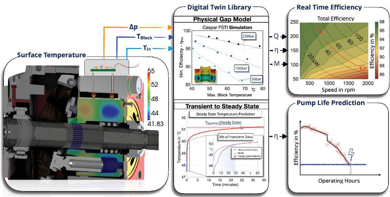
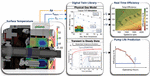
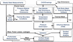
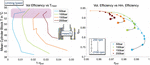
Figure 1 Real time efficiency measurements utilizing the cylinder block surface temperatures and a digital twin library.
The primary objective of this paper is to demonstrate that a digital twin, based on gap simulations, is capable of accurately predicting the relationship between a pump’s efficiency and its cylinder block temperature, validated through real-world measurements. Specifically, the paper focuses on the temperature field of the cylinder block of a 160cc open circuit pump. Figure 1 illustrates this vision: Non-invasive surface temperature measurements, along with pressure and inlet temperature data, will be integrated into a digital twin library. This library features a temperature-efficiency look-up table generated from gap simulations. Furthermore, this paper introduces a novel method that predicts steady state temperature from short transient data, enabling real-time efficiency assessments without the typical delays associated with achieving thermal equilibrium. By providing real-time efficiency data, the system can monitor both flow and torque losses, significantly enhancing current monitoring capabilities. Tracking efficiency over time across an entire fleet allows for a clear, predictable pump life estimation. Additionally, the paper highlights important thermal boundary conditions that can further enhance the model’s accuracy by reducing the reliance on pressure sensors. This approach not only facilitates real-time efficiency tracking but also provides a foundation for predicting pump lifespan and proactively identifying potential failures before they occur.
2 Research Goal and Approach
The research goal is to develop a robust methodology for monitoring the efficiency of an axial piston pump through the evaluation of the cylinder block’s surface temperature. To achieve this, the following steps were undertaken:
1. Develop a comprehensive digital twin of the entire pump using gap simulations to establish the relationship between temperature and efficiency.
2. Validate the digital twin against real-world efficiency measurements.
3. Construct a test rig with advanced thermal probing equipment, capable of measuring both the cylinder block temperature and the fluid temperature within the displacement chamber.
4. Measure all thermal boundary conditions, including fluid temperatures, housing temperatures, and heat convection coefficients.
5. Identify significant thermal characteristics from these measurements, providing potential benefits for industrial applications.
6. Propose a practical strategy for monitoring real-time hydrostatic pump efficiency.
The simulation model was built using Caspar FSTI, serving as a predictive tool to estimate the losses occurring within the pump’s three main lubricating gaps. The ability to simulate both the temperature field and efficiency of the pump is indispensable, particularly in industrial environments where such detailed measurements are often impractical. This digital twin offers a reference point for comparing ideal conditions and nominal part dimensions, making it a valuable tool for assessing pump efficiency, predicting lifespan, and understanding wear-in behaviors.
Several enhancements were introduced to the model, including adjustments for component wear, part tolerances, and improved thermal boundary conditions. The influence of component wear is demonstrated in this paper, while other elements, such as the measured heat convection coefficients, fluid temperature and the inclusion of part tolerances, have been previously published in conference papers by the author [5, 6].
The digital twin’s predictive capabilities were validated through efficiency measurements conducted on an unmodified pump. These baseline measurements served as benchmarks for comparison with the simulation results, ensuring the model’s accuracy in predicting efficiency and confirming that subsequent modifications did not negatively impact pump performance.
Following validation, the cylinder block of the test unit was modified with the strategic placement of temperature sensors at locations identified through the simulated temperature field analysis. These sensors provided detailed insights into the temperature gradients across the cylinder block during operation. A coupled Finite Element Method (FEM) analysis, utilizing the variant piston pressure field from the gap simulation, was employed to estimate the cylinder block’s lifetime under various sensor configurations. This was necessary to ensure fatigue resistance throughout the duration of the measurements, as the structural integrity of the block had been compromised by the drilling of sensor holes and cable channels. To both power and record the data of rotating sensors an innovative telemetric system was developed in-house, which enabled both high-bandwidth measurements in high-speed rotational environments with more than 30 channels. The system, previously utilized for temperature and pressure measurements in turbine applications [7–9], was pivotal in confirming the predicted temperature-efficiency correlations.
The test rig also yielded valuable transient temperature trends, previously unattainable due to the simulation model’s reliance on thermal steady state conditions. These transient trends enabled the development of a transient-to-steady-state conversion, which allows for steady-state temperature predictions using just 30 seconds of data. This breakthrough significantly enhances the ability to assess pump efficiency in real-time, eliminating the need to wait for the system to reach thermal equilibrium.
To further refine the model, high-speed pressure and temperature measurements were simultaneously captured from the fluid inside the displacement chamber, in conjunction with the cylinder block temperature measurements. This provided unprecedented insights into the complete thermal dynamics of the cylinder block and the rotating assembly within an axial piston pump.
3 Literature
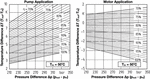
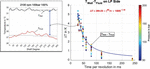
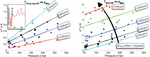
In the past numerous researchers focused on the thermal analysis as well as the study of the lubricating gaps in hydrostatic machines. The first comprehensive thermal investigations that linked temperature with efficiency have been published by Schlösser and Witt in 1976 [10, 11]. In their studies the stationary thermal behavior of the fluid line temperature was successfully linked with the efficiency of pumps and motors, as shown in Figure 2. The concept was confirmed both in theory, using entropy and enthalpy terms, and measurement. The practicality of their findings is lacking the time aspect, e.g. the amount of time it takes for the line temperatures to reach steady state conditions and the distinction of where these losses occur, but nevertheless pave the way for a comprehensive thermal – efficiency model.
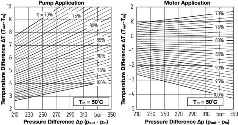
Figure 2 Total efficiency of the hydrostatic machine at steady state line conditions [12].
To understand where these losses occur and under what conditions, a gap analysis is necessary. In the era preceding advanced computational modeling, the fluid gaps of these machines were studied empirically, mostly with highly modified pump components on specialized test rigs. The body of scholars contributing to this domain is vast, hence only a short overview will be given. Test rigs that analyzed the micro movement and pressure distribution gave insight on the necessary gap heights, surface finish and analytical design methods [13–20]. As most of these empirical studies were not performed in an actual pump environment, efficiency tests were infeasible. In the past two decades sensors and electronics have allowed for a less invasive measurement of both gap height and temperature in fully functional pumps [16, 17, 21–27]. However, the findings mostly focused on the validation of simulation models, rather than a pump analysis. Most investigations were confined to a singular lubricating gap, missing a holistic analysis of the pump.
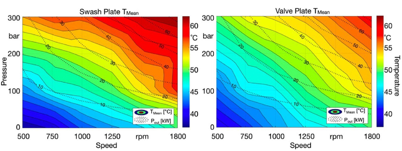
Figure 3 Simultaneous temperature measurements at valve plate and swash plate [1].
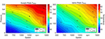
In an effort to tackle this problem the author has built a test rig where two out of the three lubricating gaps were monitored both in gap height and temperature [1, 28, 29]. The work gave a unique insight into the thermal conditions in a pump over its entire working regime, demonstrating the unique behavior of each gap, as shown in Figure 3.
The findings also showed that there is a direct correlation between temperature in the gap and its power loss, which was derived from the measured gap heights (see Figure 4). While the trend between the piston and the cylinder block was captured exclusively in simulation, it mirrored parallel trends, e.g., an apparent pattern across varying pressure levels. This research endeavors to integrate the final missing link: the measurement of the cylinder block’s temperature. In doing so, it paves the way for an exhaustive thermo-energetic dissection of the lubricating gaps.

Figure 4 Predicted power loss vs temperature at all three lubricating gaps [1].
4 Digital Twin Development and Simulation Prediction
This chapter outlines the development of a digital twin for the axial piston pump and details the methodology used to predict temperature and efficiency behavior under real-world operating conditions. The emphasis is on building a high-fidelity model using the Caspar FSTI simulation tool, which allows for detailed gap simulations. The model’s accuracy is validated through both simulation results and experimental measurements, ensuring its reliability in capturing the thermal and efficiency dynamics of the pump.
4.1 The Test Pump
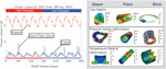
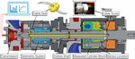
For the purposes of this research project, an Inline/Hawe-V30E 160cc axial piston pump was selected as the test unit. This pump operates with a maximum pressure of 350 bar and a maximum speed of 2100 rpm, making it suitable for investigating a wide range of operational conditions. Due to its size, the pump provides enough space for the necessary sensor integration required for precise measurements.
The pump features a traditional design, characterized by a maximum swash plate angle of 15, which makes the results generalizable to other axial piston pump models from various manufacturers. One of the few distinctive features of this pump is the unique dual surface slipper design, as opposed to the typical three-surface configuration, and a very narrow gap between the housing and the cylinder block. The narrow gap plays a crucial role in the heat transfer mechanisms within the pump, affecting both temperature and efficiency due to increased churning losses.
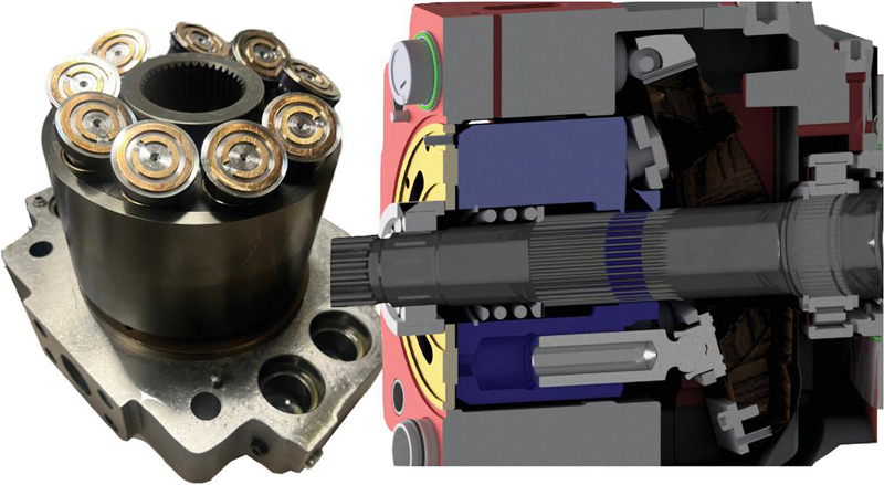
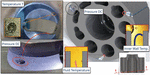
Figure 5 The rotating kit of the 160cc axial piston pump both in photograph and cross section.
4.2 Simulation Setup Using Caspar FSTI
To model the pump’s performance and develop a digital twin, the Caspar FSTI simulation software was employed. Caspar FSTI is widely recognized for its capability to simulate fluid-structure interactions (FSI), predict efficiency, and simulate the temperature evolution in axial piston pumps.
The software enables a detailed numerical analysis of the pump’s main lubricating gaps, which are critical for determining its efficiency and temperature behavior. The core losses, such as viscous friction and leakage, are modeled, and their effects on the component temperatures are thoroughly investigated. Initially, the simulations were based on nominal CAD data, which were later refined by real-world measurements to improve model accuracy. The software tool is commercially available and was validated for various pumps from different manufacturers and individual gaps by a number of indepndent researchers [1, 24, 26–28, 30, 31].
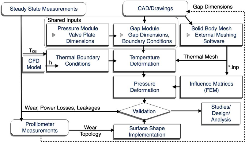
Figure 6 Typical Workflow for building a digital twin using caspar FSTI.
A typical workflow for creating a digital twin in Caspar FSTI is illustrated in Figure 6. The process begins with extracting the pump’s dimensions from technical drawings and CAD data. These valve plate dimensions allow the Pressure Module to calculate the pressure profile and resulting forces and moments. These values are then fed into the Gap Module, which calculates the pressure, temperature, and dynamic gap movements numerically, considering fluid-structure interactions. There are a number of other steps necessary such as creating the solid body meshes that allow for the temperature and pressure deformation, setting the correct thermal boundary conditions such as fluid temperatures, initial component wall temperatures and the correct surface toplogy. As articulated in Figure 6 some boundary conditions need to be either derived from CFD models, scaled from other pumps, or as was done in this case measured. In case some information is unknown, such as wear or fluid temperatures due to lack of test data, an iterative approach can be taken. For example the resulting power loss of the an initially guessed for the fluid temperatures in drain and high-pressure, can be used in a thermal model to calculate the expected outflow temperatures. Then the simulaiton neeeds to be re-run with the newly calculated temperatures. This process needs to be repeated until the temperatures converge. Such thermal models can be found in literature [32, 33].
4.3 Boundary Conditions and Simulation Validation
For accurate simulation results, the boundary conditions must reflect the actual operating environment of the pump. Stationary measurements provided the essential data for these conditions, including operating parameters like inlet, outlet, and leakage temperatures. Heat transfer coefficients and initial temperatures for all pump surfaces were also defined. These coefficients were either obtained through computational fluid dynamics (CFD) tools, from other pumps using scaling laws or determined from empirical data.
Elastic deformations due to both temperature (TEHD) and pressure (EHD) are included in the simulation by generating solid meshes for the components. These meshes, created using external tools like Hypermesh or Ansys, are imported into Caspar in the Abaqus format for thermal simulations. For pressure-induced deformations, an Influence Matrix is created based on finite element method (FEM) calculations, defining the relationships between surface nodes and pressure loads. These matrices serve as lookup table to speed up the simulation time. Their function is described in detail in [24, 34].
The simulation predicts component deformation at every time step and recalculates the temperature field at the end of each pump revolution. Caspar FSTI’s strength lies in its ability to account for both thermal and pressure-induced deformations, resulting in highly accurate predictions for power losses, gap heights, and the overall temperature distribution. An example of the power losses for the pump, before any wear was introduced, is shown in Figure 7. The simulation results indicate that the slipper exhibits the highest losses at this particular operating point, while the valve plate/block and piston/bushing sealing gap experience significantly lower, yet roughly equal, losses. The tool’s capability to accurately predict how these partial power losses fluctuate under varying operating conditions has been described and validated in [1].
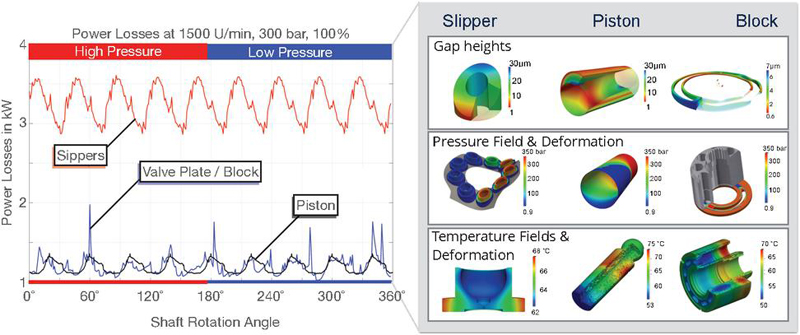
Figure 7 Typical Caspar FSTI outputs, including pressure fields, gap heights, deformations, and temperature distributions.

Figure 8 Modeled oil properties of typical HLP46 hydraulic oil.
Both local and global influences of pressure and temperature are not only a result of part deformation but also stem from changes in the fluid’s properties. In this study, HLP46 (ISO VG46) oil was used, with the tool accounting for variations in key fluid properties such as bulk modulus, density, and kinematic viscosity. These properties are recalculated at each time step for discrete fluid volumes in the gap. Figure 8 illustrates how these fluid properties fluctuate with changes in pressure and temperature.
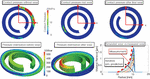
4.4 Predicting Wear to Improve Thermal Forecast
In order to forecast the correct pump efficiency, it is crucial to include the worn-in pump parts, otherwise the simulation will overpredict the losses and temperature levels. Surface measurements are not always available; thus this section will illustrate how the simulation can predict the surface run-in and demonstrate the dramatic change in efficiency an temperature level, due to just a few micrometer of material abrasion. Figure 7 shows that the simulation predicts a much higher power loss at the slipper/swash plate interface for the given operating condition. The inputs were nominal part dimensions of the slipper along with a perfectly flat surface assumption. With these assumptions the simulation predicted contact during the high-pressure stroke not only for this pressure and speed level. Figure 9 (left) shows the predicted slipper wear potential for various operating conditions. The speed increases from left to right, indicating that at low speed and high pressure as well as at high speed the slipper tends to wear in. In the plot on the top right, the average contact pressure in the fluid gap between slipper and swash plate is shown over one shaft rotation for 2100 rpm and 300 bar. The simulation predicts contact during the high-pressure stroke between 0–180. On the bottom right, contact pressure, fluid height and the pressure in the gap are shown for , illustrating the contact location.
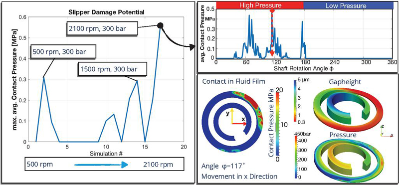
Figure 9 Slipper contact for various operating points.
The x-direction illustrates the movement direction, while the y-direction is the radial outwards direction, in which the centripetal force acts. As a result of this force slipper is tilted towards the inside edge, as indicated by the 3D gap height in the top right corner. Due high loads and an inadequate hydrodynamic pressure build-up, the gap height is very low during this point, causing a contact pressure on the leading edge of the slipper. This slipper has two sealing lands, the outer is the main seal, where the pressure drop from the pocket occurs, while the inner land is for hydrodynamic and structural purposes. Before the wear-in the slipper orientation is not beneficial for the inner edge, causing a low hydrodynamic built up. After the wear the slipper tilt changes, leaning more on the trailing edge.
This is illustrated by the 3D pressure field on the bottom of Figure 10. This figure shows the contact pressure for three wear stages on the top half: No wear, wear after 2 iterations, and contact prediction after the final wear profile is reached. The bottom right graph shows the material removal on the main sealing land as predicted by iterative simulation approach compared to a measured profile using a profilometer. The predicted wear matches reality quite well, indicating a 2 m wear of at the outer edge of the sealing land. The used wear model, which uses the contact pressure and predicts the material removal in m, is described in detail in [3].

Figure 10 Wear prediction at the slipper using Caspar FSTI at 2100 rpm and 300 bar.
On the bottom of Figure 10 is the 3D gap height with the pressure field for the non-worn slipper and the slipper with wear at 2100 rpm and 300 bar. The less then 2 m rounding of the sealing land edge causes a shift in orientation, allowing the inner land of the slipper to build up a significant amount of pressure. This stabilizes the slipper, increases gap height to more efficient levels and prevents further wear. This change in orientation and gap height produces less viscous friction.
The impact of this 2 m gap edge wear can be seen in Figure 11 for an operating condition of 1500 rpm and 300 bar. The change in tilt and resulting higher gap heights causes the power losses to decrease by 3 kW and the torque loss by more than 50%. The temperature level of the swash plate is greatly affected by the reduced power losses, dropping by more than 100C, which in turn reduces the leakage and retrospectively the entire cylinder block temperature. The temperature field of the swash plate is shown in Figure 12. This example demonstrates the importance to adequately model each gap, as they are all connected either directly or indirectly through the surrounding oil in the case.
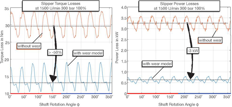
Figure 11 Simulated torque and power losses with and without wear modeled.

Figure 12 Predicted temperature with and without wear model at 1500 rpm and 300 bar.
Similar to the shown slipper case study, each surface pairing was modeled, and wear was either predicted or measured and then accounted for. After all wear is accounted for, the entire operating range of the pump is simulated and analyzed. The results are presented in the following chapter.
4.5 Prediction of Power Losses and Efficiency
The Inline-V30E 160cc pump’s simulation revealed how various gaps influence the temperature field and power losses. The Caspar FSTI model was capable of simulating the temperature and power losses across all three main lubricating gaps: the slipper, valve plate, and cylinder block.
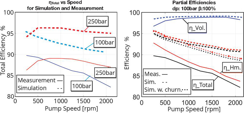
Figure 13 Efficiency prediction of the digital twin compared to the measurement.
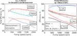
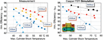
The simulated pump efficiency at full displacement across all speed levels is compared to the measurement in Figure 13 for two pressures. The simulated efficiency is based on the worn-in pump parts and the worn surface shapes. On the left, the total efficiency at 100 bar and 250 bar is plotted across the pump’s speed range, with measured values represented by solid lines, color-coded according to the pressure. Overall, the simulated efficiency follows the measured trend closely, though it tends to be slightly higher than the actual values. This discrepancy is expected, as certain loss sources, such as shaft bearing losses and the setting system, are not fully accounted for in the simulation. Nevertheless, when comparing the overall trend, there is a strong correlation between the simulation and measurement at both pressure levels. The simulation correctly predicts the drop off at 250 rpm and 250 bar, as well as the trend with speed at both pressure levels. This low-speed region showed the most significant changes when comparing simulation with and without wear. The differences in the efficiency magnitudes can be explained by the right side of the figure. Here the partial efficiencies at 100 bar are shown for both measurement and simulation. As can be seen the volumetric efficiency is matched quite well. The discrepancy results in the hydrodynamic efficiency, which directly correlates to friction and torque losses. The simulation model predicts the losses in the lubricating gaps of the rotating group only, neglecting additional frictional losses. This claim can be supported by the fact, that the difference between the measured and simulated hydromechanical efficiency increases with speed, as the churning losses increase with the exponential of the speed, as shown in published models and measurements [35–37]. According to the CFD simulations the churning losses for this pump at 2100 rpm are close to 5.5 Nm. This amounts to about 2% additional losses in the hydromechanical efficiency at 100 bar, which is in agreement with the model of Bing [36]. Factoring in these churning losses in the hydromechanical efficiency result in the dotted line shown in the right figure.
When accounting for all parasitic losses, such as bearing, churning, and setting system losses, the digital twin can accurately predict the overall pump efficiency, both in trend and magnitude. This is demonstrated in Figure 14, where the measured total efficiency at 100% displacement is shown on the left, and the simulated efficiency with parasitic loss modeling is shown on the right. The efficiency is plotted for various speeds and pressures, with color contours representing the efficiency values. Both plots are closely aligned, with their respective color bars indicating very similar efficiency ranges. The power output curves, represented by the black lines, further highlight the correlation between measurement and simulation. The digital twin successfully captures both the overall trends and finer nuances in efficiency. Some minor discrepancies occur at extreme operating conditions – such as very low speeds at high pressure and very high speeds at low pressure – likely due to simplifications in the shaft bearing model [38]. However, these parasitic losses can be calculated with little effort when compared to the gap simulation model. The gaps highly unpredictable behavior is captured quite well when comparing the overall shape of the efficiency field. This example demonstrates that the digital tiwn is high accuracte in predicting total efficiency and its components, including volumetric and hydromechanical losses.

Figure 14 Efficiency prediction of the digital twin compared to the measurement.
4.6 Predicting Cylinder Block Temperature
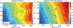
Once the pump’s efficiency is accurately predicted, it follows that the temperature within the cylinder block should align accordingly. However, achieving precise temperature and efficiency predictions requires precise boundary conditions. Factors such as correct part dimensions, heat convection coefficients, material properties, and wear significantly influence temperature behavior. This is illustrated in Figure 15, which shows both the maximum and mean temperatures of the cylinder block across various speeds at 100 bar and 100% displacement.
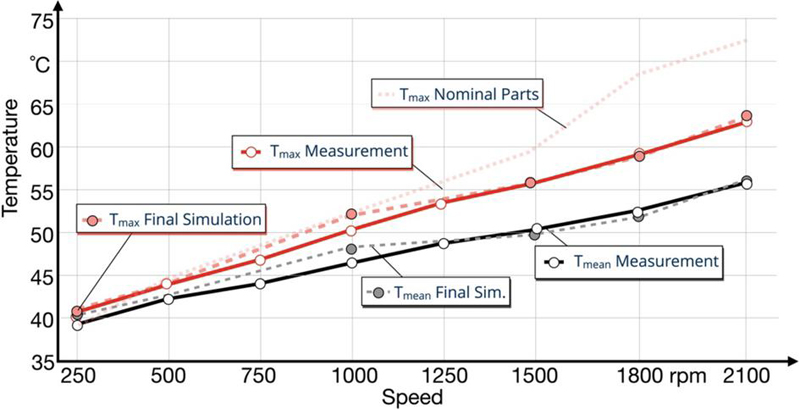
Figure 15 Final output of the digital twin compared to measurement at various speeds at 100 bar and 100% displacement angle.
Figure 15 presents a comparison between the measured and simulated temperatures. The solid red and black lines represent the measured maximum and mean temperatures, respectively, while the dashed lines correspond to the simulation results. The top curve shows the maximum temperature (T) of a preliminary simulation model. Here the temperatures deviate quite significantly at high speeds, which is primarily due to nominal part assumptions and no wear. After considering actual part dimensions, gathered using profilometer measurements, both T and T closely matching the measured data.
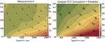
After achieving the correct boundary conditions, the simulation closely matches both efficiency (as demonstrated in Section 4.5) and temperature. This is illustrated in Figure 16, which shows the average temperature field at 50% displacement.
In the contour diagram the simulated temperature fields is varied across various speeds and pressures. On the left, the measured average temperature (T) is plotted, while the right figure represents the simulated temperature field. The color contours correspond to different temperature levels, with cooler regions in blue and warmer regions in red, reflecting the temperature distribution across the cylinder block.
Both figures show a consistent temperature increase as speed and pressure rise, with close alignment between the measured and simulated data. The power output (P in kW) is indicated by contour lines in both figures, showing how temperature does not directly correlates with power, as the lines cross. The close match between these temperature fields highlights the simulation’s accuracy in predicting thermal behavior, ensuring that both efficiency and temperature predictions align under the given boundary conditions.
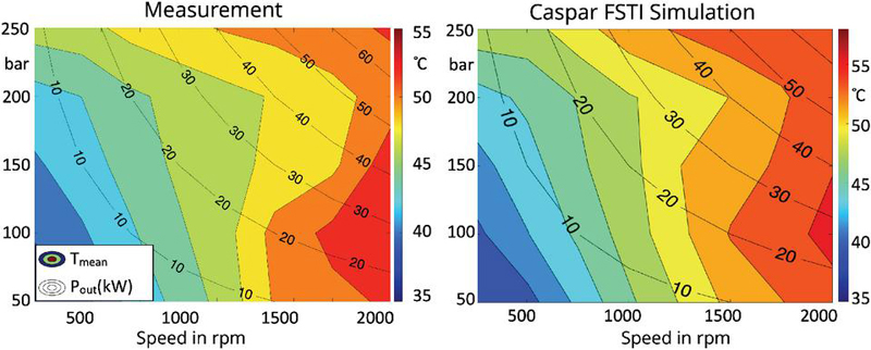
Figure 16 Measured and simulated average cylinder block temperature field at 50% displacement.
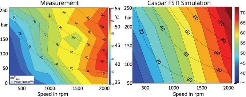
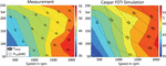
Figure 17 Measured and simulated maximum cylinder block temperature field at 100% displacement.
Predicting the maximum temperature level is more challenging than the average temperature due to its sensitivity to slight deviations in geometry or minimal wear that may not have been fully accounted for. Despite these challenges, the general trend at 100% displacement is illustrated in Figure 17.
The left panel displays the measured maximum temperature (T), while the right panel shows the corresponding simulated maximum temperature field. The color contours represent temperature levels, with cooler areas depicted in blue and progressively warmer areas in red. The temperatures are plotted against the pump’s speed across a range of operating conditions. Additionally, power loss (in kW) is overlaid in contour lines in the left panel, providing insight into how power losses correlate with maximum temperature.
While the overall trend of increasing temperature with rising speed is consistent between the measurement and simulation, discrepancies can be observed in the exact temperature values, especially in high-speed regions. These deviations are likely due to unaccounted factors such as slight geometric variations or wear that significantly impact localized peak temperatures. Nevertheless, the simulation captures the general temperature distribution, demonstrating the model’s ability to predict maximum temperature trends under real-world conditions.
4.7 Simulated Correlation Between Efficiency and Cylinder Block Temperature
Building on the results from Sections 4.5 and 4.6, where we successfully demonstrated that the digital twin could accurately simulate both efficiency and temperature, an interesting correlation between these two parameters emerges. The ability to predict both efficiency and temperature provides deeper insights into the pump’s performance under various operating conditions. Understanding how these factors influence each other is crucial for optimizing pump behavior.
By combining these two aspects – efficiency and temperature – a strong correlation can be observed, which forms the basis for the proposed condition monitoring system. Elevated cylinder block temperatures affect the pump’s efficiency by influencing oil properties such as viscosity (as shown earlier in Figure 8), which, in turn, impacts leakage and gap height. These dynamic changes influence the overall efficiency, highlighting the importance of accurate temperature predictions in evaluating pump performance.
Figure 18 presents the simulated correlation between the maximum cylinder block temperature and the volumetric efficiency () on the left, and the hydromechanical efficiency () on the right. The x-axis represents the maximum cylinder block temperature, while the y-axis shows the respective efficiencies. Each circle in the plot corresponds to a specific operating condition, with color-coded pressure levels: blue for 100 bar, red for 200 bar, and green for 300 bar. The dotted lines represent linear fits for each pressure level, clearly demonstrating how efficiency varies with temperature.
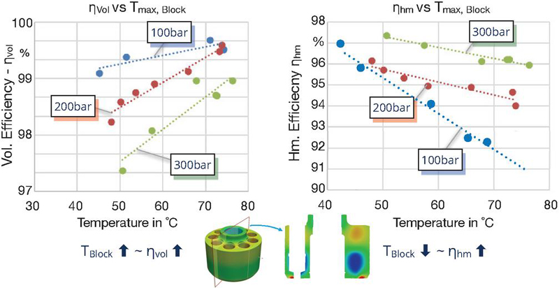
Figure 18 Simulated correlation between efficiency and cylinder block temperature.
As seen in the left panel, volumetric efficiency exhibits an upward trend, especially at higher pressures. This is likely due to the cooling effect of leakage flow, where increased leakage leads to heat being carried away from the lubricating gaps, thereby reducing the part’s temperature. Consequently, higher volumetric efficiency corresponds to elevated temperatures, as less leakage results in less heat dissipation. Conversely, in the right panel, hydromechanical efficiency shows an inverse relationship with temperature. Higher hydromechanical efficiency corresponds to lower power losses due to friction, which in turn results in lower temperatures.
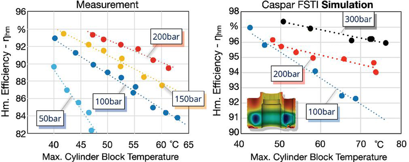
Figure 19 Measured and simulated correlation between Hm. efficiency and cylinder block temperature at various pressures.
Figure 19 illustrates the comparison between the measured hydromechanical efficiency (left) and the simulated results from the digital twin (right). The x-axis represents the maximum cylinder block temperature, while the y-axis shows the hydromechanical efficiency (). Each dataset is color-coded by pressure levels: blue for 100 bar, red for 200 bar, and yellow/orange for pressures between 50 and 300 bar.
The measurement results confirm the linear relationship between temperature and efficiency across discrete pressure levels. Additionally, the data highlights a change in slope at lower pressures, where efficiency is less sensitive to temperature increases. This behavior is mirrored in the simulation results, where a similar trend and pressure-dependent slope changes are captured.
Differences in efficiency height between the measured and simulated data can be attributed to two main factors: the neglect of parasitic losses in the simulation (such as bearing and churning losses), and slight deviations in the maximum temperature caused by local wear effects that may not be fully captured in the simulation. However, despite these differences, the overall trend matches well, proving that measuring the cylinder block’s temperature allows for a reliable prediction of the pump’s efficiency.
In conclusion, the digital twin model developed through gap simulations demonstrates a robust capability to predict both temperature and efficiency, accurately capturing real-world behavior under varying operating conditions. The simulations not only predict overall efficiency but also break down the components of volumetric and hydromechanical efficiency in relation to temperature. This level of predictive power opens new possibilities for condition monitoring and performance optimization in axial piston pumps.
The next chapter describes the test rig setup, which was used to validate the digital twin model and conduct detailed temperature and efficiency measurements.
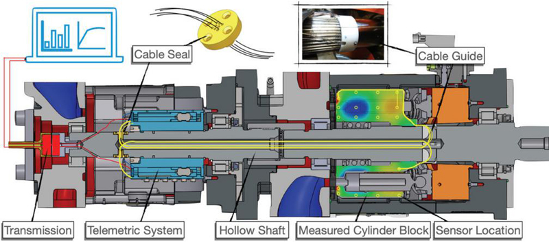
Figure 20 Measurement set up.
5 Analysis of Temperature and Pressure Dynamics
To validate the predicted temperature-efficiency trends, it is necessary to measure the cylinder block temperature in a regular pump setting, without modifying crucial pump components, as has been done in the past [21, 26, 39]. To accomplish this, a special telemetric system was used, which can accurately measure a large number of sensors simultaneously. The system was originally developed to measure temperature and pressure in high speed turbine applications within an accuracy of 0.1K. The system was adapted to measure 24 thermocouples and 4 heat convection coefficient sensors.
The set up can be seen in Figure 20, where a tandem pump arrangement was used to mount and house the telemetric system to the 160cc open circuit pump, while the test pump is shown on the right, with the tested cylinder block highlighted. The sensor locations and temperature field are illustrated, with the exact sensor locations shown in Figure 22. The sensor cables are guided from the cylinder block through hollow shafts using 3D printed parts to guide the cables during pump assembly. In order to seal the case properly the cables were individually guided through a cable seal, that was then sintered shut. The used thermocouples were of type K with metal mantle, which allowed them to be sintered into the cylinder block. The telemetric system converts the analog temperature signals to digital bits that can be transmitted wirelessly to the acquisition system. The power is also transmitted through this brushless system. This set up allows for a very reliable and accurate measurement, not only of temperature but also other signals. In future publications simultaneous pressure and temperature measurements will be shown, that were recorded using this set up.
Next to the cylinder block’s temperature, the pump is also monitored holistically with an array of sensors, as shown in Figure 21. Each fluid line is equipped both with pressure and temperature sensors, where the temperature is recorded with industrial as well as high accuracy thermistors. The housing of the pump is equipped with 5 temperature sensors and a thermal camera recorded the temperature distribution. As the run-in process and the local temperature are in correlation, the pump was also monitored for particles emitted. The suction line was also equipped with a transparent section that allows for visual inspection of air bubbles, to ensure for a cavitation free operation.
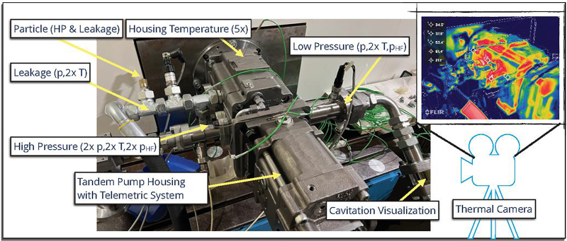
Figure 21 External sensors on the test pump.
5.1 Cylinder Block Temperature Measurements
Figure 22 showcases a sample result for a high-speed operating condition. Here, the simulated outcomes (on the left) can be compared to the measurements (on the right and in the table). For the specific operating parameters of 2100 rpm, 200 bar, and 100% displacement, the pump remained inactive for over 24 hours, essentially reverting to room temperature before initiating the test. Following this, there was a gradual ramp-up, with speed escalating from 0 to 2100 rpm within approximately 10 seconds and pressure surging from 0 to 200 bar within a similar timeframe.
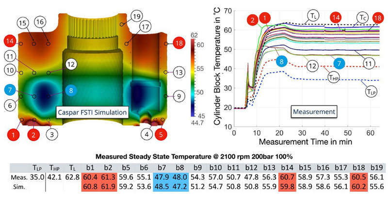
Figure 22 Measured and simulated cylinder block temperatures at 2100 rpm, 200 bar and 100% disp.
One notable observation is the swift temperature response in the cylinder block, registering changes in 15 s. However, attaining thermal equilibrium across the entire pump – where all components stabilize, and the desired inlet temperature is met (with a margin of 1K) – takes close to an hour. It should be noted that this time frame corresponds to a cold start, condition changes when the pump reached operating temperatures usually reach thermal equilibrium within 10–20 min. All measurements were aimed to be taken at 35C inlet. Small deviations were later corrected to make the results comparable between operating conditions.
Looking at the measured temperature distribution (right) and the simulated (left) in Figure 22, a good match between simulation and measurement can be seen. The predicted 15 K temperature difference in simulation matches almost the 13.5 K measurement. The sensors were placed 5 mm away from the bottom cylinder block surface, as FEM fatigue calculations predicted a negative trend drilling the holes any closer. This could explain the difference in the maximal temperatures. The highest temperature is registered at sensor 2. These high temperatures at the bottom of the block predict higher viscous losses at the valve plate interface and the other high temperatures are at the top of the cylinder block (sensor 14 & 18), close to the top of the piston / bushing pairing. The piston has a high inclination at these speeds and pressures with its lowest gap height at the top of the bushing, explaining the hot spot. The low spots are at sensor 7 and 8, which are the closest to displacement chamber, which acts in a cooling manner. Sensor 20 was placed outside of the block directly in the leakage oil around the block. It is even hotter than the block, predicting that the hottest region is in fact in the gap and that the block is heated also from the surrounding oil and not just from the gaps.
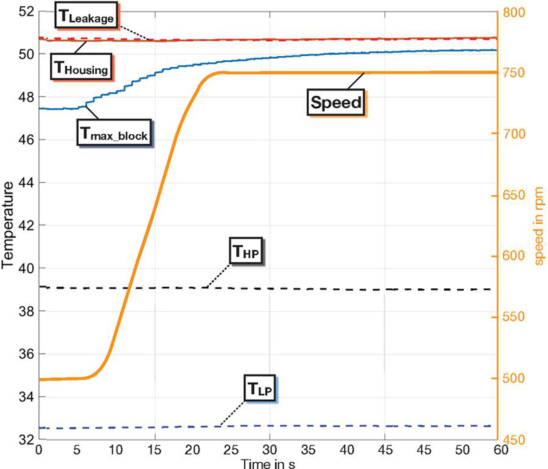
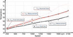
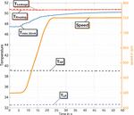
Figure 23 Temperature response rate of the cylinder block.
To demonstrate that the cylinder block is better suited for the thermal monitoring as compared to the fluid temperature or the housing, Figure 23 should be inspected. It shows a speed change from 500 to 750 rpm during warm conditions and the corresponding fluid temperature in the ports, housing temperature and the block temperature. The maximal block temperature (T) has an instant reaction to the speed change, rising 3C in 10 s. Contrarily, other fluid and body temperature readings, such as those of the inlet, outlet, housing, and leakage, remain largely consistent in the given time frame despite the speed variation. This emphasizes the significance of the cylinder block temperature and underscores the advantage of in-pump measurements.
Preliminary studies suggest that this immediate temperature spike can potentially be harnessed to predict steady-state temperatures, paving the way for a more industrially relevant monitoring approach. Nevertheless, given that the simulation resides in a steady state, achieving this state in real-time measurements is paramount for meaningful comparisons.
5.2 Measuring the Thermal Boundary Conditions in the Displacement Chamber
In the previous chapter, the setup for measuring the block temperature was described, along with insights from transient data. This chapter expands on those findings by detailing the setup and results from the high-speed pressure and temperature measurements inside the displacement chamber. These measurements provide a deeper understanding of the thermal boundary conditions, which are critical for accurately predicting the pump’s performance.
Figure 23 illustrates the sensor placement for both temperature and pressure measurements within the displacement chamber. One temperature sensor was positioned in direct contact with the fluid inside the displacement chamber, allowing it to measure the real-time fluid temperature during operation. Another temperature sensor was embedded slightly differently – due to the wire length protruding – resulting in it being in contact with the inner wall of the chamber, which introduces a slight variation in the measurement. This setup captures the difference between the fluid’s temperature and the chamber wall temperature, providing critical data for understanding the heat transfer dynamics. The temperature sensors are Type K (sheathed thermocouples) with an accuracy of 0.1 K and a repeatability of 0.05 K.
Additionally, one pressure sensor was strategically placed within the chamber to capture high-speed pressure fluctuations during operation. This sensor was mounted in the kidney, while the temperature sensors were located near the corner of the chamber. The miniature pressure sensor is of type EPB-B0 diaphragm from Althen. It’s FSO is 350 bar and has a repeatability of 0.25% FSO. This layout ensures comprehensive monitoring of both temperature and pressure dynamics in real time, offering a complete thermal picture of the rotating assembly.
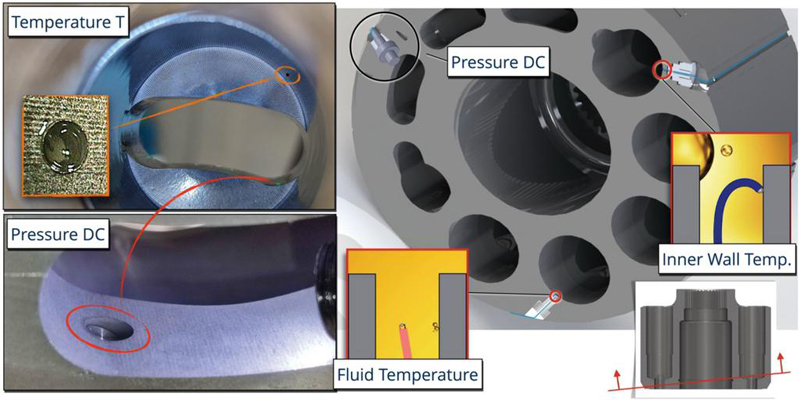
Figure 24 Sensor placement for temperature and pressure measurements inside the displacement chamber. The left image shows the positioning of the pressure sensor (bottom) and temperature sensor (top) on the cylinder block. The right shows the relative placement.
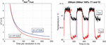
Figure 25 illustrates the transient pressure and thermal behavior within the displacement chamber at 250 rpm, 200 bar, and 100% displacement. The fluid temperatures in the displacement chamber are displayed in red (T) and black (T). The pressure signal clearly identifies the high-pressure zone (0–180) and the suction zone (180–360). As the piston begins its compression stroke, the pressure rapidly increases to 200 bar, and both the wall and fluid temperatures rise with a slightly delayed response reaching its peak at . Around this point, the piston connects to the high-pressure kidney. At this low speed, the temperature remains stable throughout the rest of the high-pressure stroke, indicating that the peak temperature has been reached. During this phase, the wall and fluid temperatures converge, while in the low-pressure stroke, they diverge.
At the bottom dead center (BDC) is reached, meaning the piston is fully retracted into the bore. Here, the low-pressure stroke begins. As soon as the pressure drops, both wall and fluid temperatures decrease, with the fluid temperature dropping more significantly – by approximately 1.2 K lower than the temperature on the high-pressure side. However, the fluid temperature does not return to the inlet temperature (37.6C, measured just before the pump port), suggesting heat exchange within the low-pressure port. A temperature sensor in the endcase records a steady-state port temperature of 41.6C. The outlet temperature of 40.1C matches the wall and fluid temperatures observed during the high-pressure stroke.
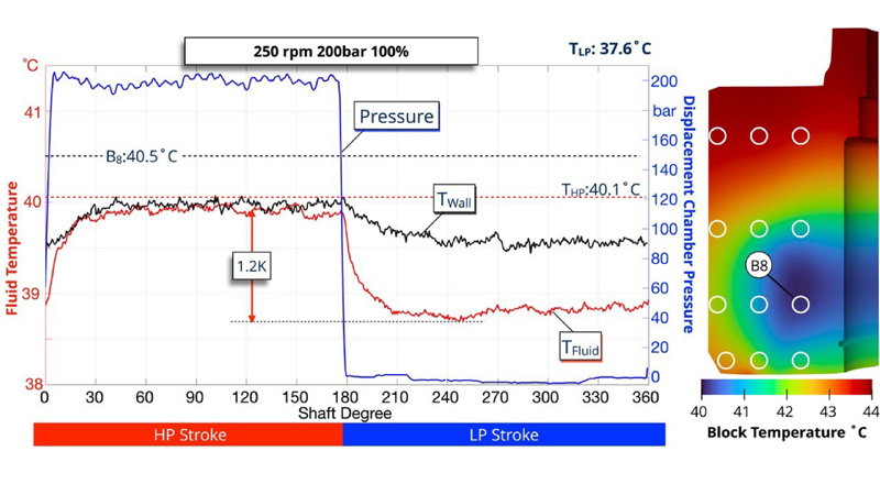
Figure 25 Wall layer, fluid, and cylinder block temperatures at 250 rpm, 200 bar, and 100% displacement.
The right side of Figure 25 shows the measured cylinder block temperature field and the location of several sensors. Sensor 8 (B8) is highlighted as it is closest to the displacement chamber wall, representing the lowest temperature detected on the block. In this scenario, the cylinder block temperature is slightly higher than both the wall and fluid temperatures, indicating a heat transfer from the block to the fluid, with the fluid simultaneously cooling the block. Notably, these temperature differences vary at higher speeds, as will be demonstrated later in this chapter.

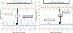
Figure 26 High-speed temperature response (left) and temperature difference between fluid and wall (right) as a function of time per revolution (ms).
As demonstrated at low speed, there is a difference between wall and fluid temperature both during the suction and delivery strokes. The next section provides a detailed analysis of how these temperature differences vary with changing conditions. Figure 29 illustrates the wall and fluid temperatures at 2100 rpm, 100 bar, and 100% displacement (left) during a cold start, with an inlet temperature close to room temperature at 25C. Notably, the temperature gradients of both fluid and wall remain consistent even after reaching steady-state conditions with an inlet temperature close to 35C. The trend here differs significantly from the low-speed plot shown in Figure 25. While the fluid temperature (red line) rises during the high-pressure stroke, it does not level off and instead reaches its peak at the end of the high-pressure stroke, suggesting that the temperature response is too slow to keep up with the high dynamic conditions.
In contrast, the wall temperature (black line) remains nearly constant throughout the revolution, indicating that the wall’s higher heat capacity dampens its dynamic response. The temperature difference (T) between the wall temperature (T) and fluid temperature (T) on the low-pressure side is shown on the right side of the figure, plotted against the time taken for a full revolution. All measurements are color-coded by pressure level, as indicated by the color bar. As observed, all measurements align closely with the shown trend line, with the corresponding equation displayed in the figure.
A similar trend line was generated for T on the high-pressure side, which follows a slightly different curve. Both trend lines are shown on the left in Figure 27. As illustrated on the right (under the same conditions as in Figure 25), the temperature difference between the wall and fluid is larger on the low-pressure (LP) side at low speeds than on the high-pressure (HP) side. This difference decreases with increasing speed, indicating that as the fluid has less time to exchange heat with the ports, the temperature differences between the HP and LP sides become more similar.
As pump speed increases, the temperature difference between the fluid and wall widens. The primary factor contributing to this heat difference appears to be the heat exchange at the suction port. The less time the fluid has to absorb heat from the endcase, the cooler it is upon entering the displacement chamber. Meanwhile, the wall temperature depends on the cylinder block temperature, which, as will be shown in the Chapter 6, is largely influenced by efficiency. Typically, the cylinder block is warmer than the fluid, resulting in heat transfer from the block surfaces to the fluid. At higher pump speeds, the fluid spends less time in the displacement chamber, absorbing less heat from the block. This reduction in internal cooling from the fluid at increased speeds is a critical factor to consider when pursuing higher pump speeds, especially in the context of electrification.
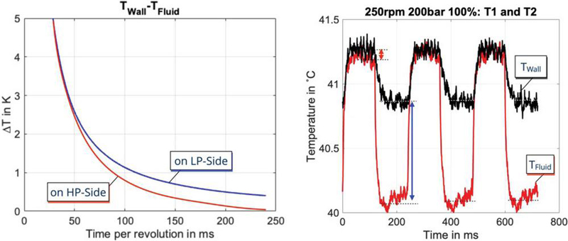
Figure 27 Temperature rise in fluid with time.
In addition to the heat transfer from the block, the fluid also gains heat through internal compression work. The next section aims to link pressure build-up with the resulting temperature increase. The first step is to understand how the pressure build-up responds to variations in speed, pressure, and displacement.
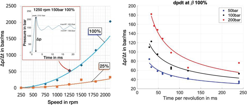
Figure 28 Pressure rise with speed (left) and temperature rise with pressure (right).
Figure 28 illustrates two key trends. On the left, the relationship between speed (in RPM) and pressure rise (p/t) is shown for two different displacements, 100% and 25% of the maximum swash plate angle. As seen, pressure rise increases nonlinearly with speed, with a notably higher rate of increase at full displacement (blue line) compared to lower displacement (orange curve). The example point at 1250 rpm, 150 bar, and 100% displacement illustrates that pressure tends to overshoot at higher speeds. This overshoot is influenced by the valve plate cross-section and the timing of grooves and pre-compression holes, which are unique to each pump design. While these specific trends may not be universally applicable to all pumps, the general behavior is likely similar.
On the right side of Figure 28, the relationship between the pressure rise rate (p/t) and the time per revolution is shown for three different pressure levels at full displacement. This figure demonstrates that the pressure rise rate depends not only on speed and flow (displacement) but also on the pressure level itself.
Figure 29 illustrates how temperature rises in relation to this pressure increase. The figure contains two graphs: the left graph shows the temperature rise over the first 30 of shaft rotation versus the maximum pressure reached within this range. Each color represents a different pump speed. The first 30 were selected because, during this interval, the piston is isolated from the high-pressure (HP) port. Once the HP connection is established, the temperature trend is heavily influenced by port flows and the HP system downstream.
In the left graph, it is clear that the fluid temperature rise is quite linear with pressure; however, the rate of this rise varies significantly with pump speed. Lower speeds result in a higher temperature jump due to the time-dependent nature of heat transfer.
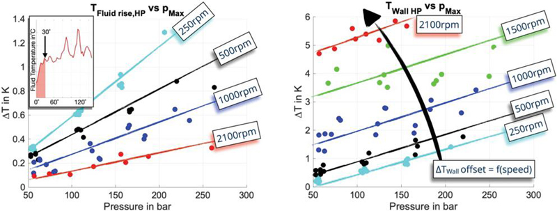
Figure 29 Temperature rise with pressure for fluid (left) and wall (right).
The right graph in Figure 29 shows the difference between wall temperature (T) and the initial fluid temperature (T), where T is the same reference point as in the left graph. Here, we observe trends associated with both pressure and speed. Unlike the fluid temperature, the wall-fluid temperature rise rate is independent of speed, although an offset exists that increases with speed – this offset was previously discussed in Figure 27
In addition to the relative temperature rise, the rate of temperature change over time is equally important. Figure 30 presents this data, showing dT/dt versus time per revolution (left) and the rate of temperature change versus the rate of pressure change (right).
On the left, the graph displays the time-dependency of the temperature rise. All measurements, including data from various displacements and color-coded by pressure levels, generally follow the same curve, with the corresponding formula listed in the graph. This indicates that time dependencies play a crucial role in the rate of temperature change within the displacement chamber, dominating the overall temperature behavior. Interestingly, while pressure rise rate varies with pressure level (as seen in Figure 28), the rate of temperature change does not show this dependency. This observation leads to the question of the correlation between temperature and pressure rise rates. The right side of Figure 30 addresses this by plotting these rates against each other, with data points color-coded by pressure level. The graph reveals a clear correlation, demonstrating a distinct dependency on pressure level
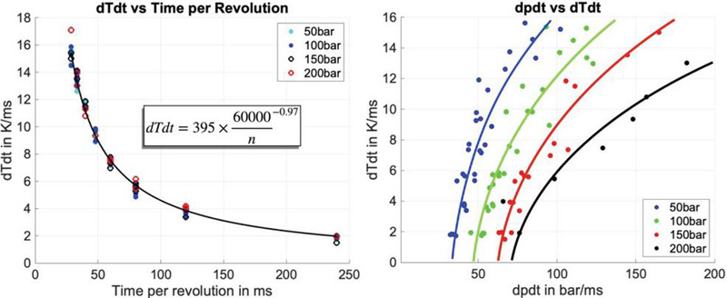
Figure 30 Temperature rise rate with time per revolution (left) and its dependency on the pressure rise rate for various pressure levels (right).
With the measured time and pressure dependencies of both fluid and wall temperatures, it is now possible to further refine the simulation boundary conditions. In particular, the wall temperature, which acts as the boundary condition between the fluid and the solid, deviates from previously assumed values due to an offset dependent on pump speed. This offset is likely influenced by the geometry of the part, with factors such as heat capacity and surface area playing a role. Although further studies are needed to thoroughly understand these correlations, this paper provides an initial step in demonstrating the dynamic temperature fluctuations that affect both fluid and wall temperatures.
To illustrate the thermal behavior within the pump, Figure 31 presents a detailed thermal map of the cylinder block, highlighting temperature distributions across the block, case, ports, and oil flow. The temperature values at various sensor points (e.g. T, T, T, and T) are displayed, revealing the temperature gradients across different pump components. Notably, the cylinder block temperature is substantially higher than the fluid and wall temperatures, reinforcing the conclusion that heat transfers from the block to the fluid and surrounding components. The temperatures shown are normalized to an inlet temperature of 35C.
The lowest temperature on the cylinder block is recorded at sensor B8, closely matching the measured fluid temperature in the displacement chamber. In contrast, the highest temperature is observed at B2, located at the cylinder block/valve plate gap. A significant temperature gradient is present at this location; sensor B3, positioned next to B2, records a temperature more than 10K lower, indicating that the block is being cooled by the displacement chamber. This gradient causes substantial thermal strain, leading to localized deformations in both the valve plate and cylinder block.
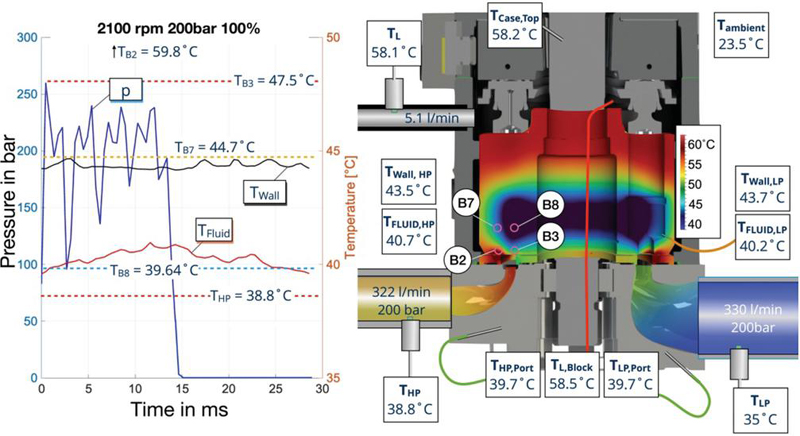
Figure 31 Complete thermal picture of an axial piston pump at 2100 rpm 200 bar 100%.
The inner wall temperature of the displacement chamber, measured at 43.5C, is comparable to the temperature at B7 but higher than the lowest solid body temperature at B8. Due to the location of temperature sensors at the bottom of the displacement chamber (illustrated by the probe on the right), wall temperatures tend to be higher in this area. Therefore, it is important to note that the shown wall temperatures represent a localized measurement rather than the entire displacement chamber boundary. Additionally, the measured fluid temperature exiting the pump is lower than the lowest block or fluid temperature measured within the pump, further demonstrating the substantial heat flow occurring within the pump’s endcase even at these high flow conditions.
This figure encapsulates the complex interactions among pressure, temperature, and pump dynamics, underscoring the importance of both transient and steady-state thermal boundary conditions for accurately predicting pump behavior.
In conclusion, Chapter 5 has illustrated the essential role of accurate thermal and pressure data in enhancing the predictive capabilities of the digital twin model for axial piston pumps. By integrating high-speed sensor measurements, this study has shown how temperature and pressure fluctuations within the displacement chamber and cylinder block influence pump efficiency under various operating conditions. The refined understanding of thermal boundary conditions – specifically the dynamic interaction between fluid and wall temperatures – has highlighted the complexity of heat transfer within the pump, emphasizing that both transient and steady-state conditions must be accounted for to achieve reliable predictions.
The findings from this chapter lay a foundation for more precise real-time condition monitoring and offer a scalable approach to predicting efficiency across different pump configurations. The ability to correlate pump efficiency with cylinder block temperature provides a promising method for condition monitoring, as it can be modeled physically with minimal data requirements. This approach allows for efficient adaptation to other pump sizes and models, utilizing accessible temperature measurements to derive valuable efficiency data for performance optimization.
In the following chapter, we explore how these temperature-based efficiency correlations can streamline condition monitoring, making it feasible to apply this methodology widely across hydraulic systems for improved reliability and predictive maintenance.
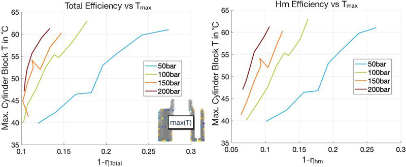
Figure 32 Measured trend between maximum block temperature and total (left) and hydromechanical (right) efficiency at 35C inlet.
6 Application and Implications for Condition Monitoring
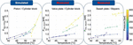
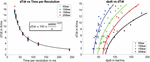
Figure 32 shows the measured relationship between efficiency and block temperature at 35C inlet temperature (as is true for all following graphs). Left in the figure is the maximum cylinder block steady state temperature T and the total efficiency loss () for each pressure region. Although the pattern isn’t strictly linear, distinct zones emerge for each pressure level. At 50 bar, the temperature increase appears to have a linear correlation with efficiency loss, suggesting that it’s primarily driven by viscous losses. However, as pressures elevate, volumetric losses start to play a more prominent role. The linear relationship between viscous losses and the temperature can be confirmed by the right graph in the figure, which shows T vs . There is a clear linear trend for each pressure level. Linear trends are easily modeled and can be very helpful in prediction. Quadratic relationships can be helpful if the entire modeling region is known. The volumetric efficiency and the temperature seem to have such a quadratic relationship, as can be confirmed by the minimal surface temperature and the volumetric efficiency in Figure 33.
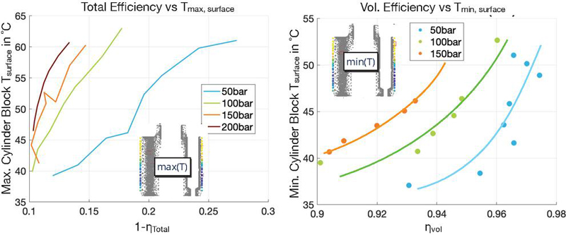
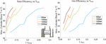
Figure 33 Total (left) and volumetric (right) efficiency trends with max and min block surface temperature.
This quadratic relationship of temperature and volumetric efficiency is shown on the right side of the figure for three pressure levels. This trend can be explained by the relationship between leakage flow increases and the gap height, as the flow increases with the height squared. Moreover, the figure underscores that merely gauging the surface temperature suffices to forecast the pump’s total efficiency. This is exemplified in the left graph, where the peak surface temperature is plotted against , revealing a similar pattern to what’s observed in Figure 32. While the measured efficiencies and temperatures are different in magnitude at the current simulation stage, they still match in trend, confirming the simulated predictions. It is worth mentioning that while the maximum surface temperature can also be correlated with the volumetric efficiency, it was better and clearer trend utilizing the minimum temperature. When correlating the T with the volumetric efficiency the trend is comparable to the one shown in Figure 34.
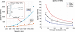
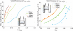
Another interesting beneficial correlating the pumps efficiency with the block surface temperature, is the prediction of the pump’s speed limit for each pressure level. In Figure 34 the plot of mean surface temperature against the loss in volumetric efficiency () reveals a noticeable deviation from the quadratic trend at specific temperatures for all pressure levels. Typically, temperature rises with an increase in volumetric efficiency. Yet, beyond a particular temperature threshold, despite a continuing rise in temperature, the volumetric efficiency starts to decline. Detailed analysis highlighted that this phenomenon emerges when the pump operates at exceedingly high speeds, nearing its maximum permissible speed.
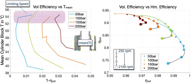
Figure 34 Limiting pump speed as per temperature and efficiency.
This observation is more pronounced when comparing volumetric efficiency to hydromechanical efficiency, as depicted on the right side of Figure 34. The plot shows each measurement point color coded with pressure and the size of the dot related the pump speed from 250–2100 rpm. During normal operation the volumetric efficiency increases with speed while the hydromechanical efficiency decreases. As can be seen this happens in a quite predictable fashion. The trend breaks at high speed when the drops while the drops as well. Notably, the speed at which this occurs varies with the pressure level: it’s more immediate at lower pressures compared to higher ones. It will be further investigated if this trend can be detected with the temperature only, but initial trends suggest that it is detectible by comparing inlet, outlet and block temperature rise. This will give the installation of a block temperature a further incentive, being able to predict speed limits in open circuit pumps can be a crucial feature.
7 Conclusion and Outlook
This study explores the complex relationship between the steady-state temperature of a 160cc axial piston pump’s cylinder block and its total, volumetric, and hydromechanical efficiency, confirming correlations that were previously suggested through simulation. Using the Caspar FSTI simulation software – renowned for its predictive accuracy in modeling axial piston pump losses – the paper demonstrates a temperature-efficiency correlation that aligns with prior findings from a 92cc pump of a different manufacturer [1], reinforcing the consistency of these relationships across various pump sizes and designs.
A key aspect of this study involved the strategic placement of 24 temperature sensors at 20 distinct positions within the rotating cylinder block, informed by insights from the simulation model. This comprehensive sensor setup allowed for the capture of detailed temperature profiles, deepening the understanding of internal thermal dynamics. Supporting this was a high-precision telemetric system, designed specifically for real-time data transmission, which enabled continuous monitoring from temperature sensors and four additional sensors dedicated to measuring heat convection coefficients.
The empirical measurements closely matched the simulated predictions across various operating conditions, successfully identifying hot and cold spots and capturing temperature ranges with a high degree of accuracy. These findings validate the simulation’s reliability while uncovering new insights into the thermal behavior of axial piston pumps, particularly as the pump approaches its speed limits – offering valuable knowledge on operational constraints and thermal implications.
To enhance understanding further, high-speed temperature and pressure measurements within the displacement chamber were conducted, capturing both fluid and inner wall temperatures and revealing significant temperature fluctuations. High sensitivity to pressure and speed was observed, which can be leveraged to refine the boundary conditions of the digital twin and potentially eliminate the need for pressure sensors in the temperature-efficiency correlations.
The demonstrated ability to predict efficiency using steady-state surface temperatures, along with the cylinder block’s rapid response to operational changes, highlights this method’s potential for real-time condition monitoring. An established method, previously published, enables the extraction of steady-state temperatures from only 15 seconds of transient temperature data from the block [5], allowing for effective monitoring even during transient conditions and expanding the practical applications of this approach. Importantly, this can be achieved without compromising the cylinder block’s durability or the pump’s overall integrity.
In future work, a wireless temperature sensor will be developed and tested, capable of being mounted directly on the surface without wired connections. Both power and data will be transmitted wirelessly through a receiver housed within the pump, advancing the feasibility of seamless real-time monitoring in axial piston pumps.
Nomenclature
| Area | m | |
| Swash plate angle | ||
| Differential temperature | K | |
| Shaft angle | ||
| Heat convection coefficient | W/mK | |
| High pressure | ||
| Speed of the pump | rpm | |
| Volumetric pump efficiency | ||
| Hydromechanical pump efficiency | ||
| Total pump efficiency | ||
| Low pressure | ||
| Temperature | C | |
| Inlet temperature | C | |
| Maximum temperature of the cylinder block | C | |
| Minimum temperature of the cylinder block | C | |
| Mean temperature of the cylinder block | ||
| Pressure | bar | |
| High frequency pressure transducer | ||
| Output power | kW | |
| Heat Flow | W |
References
[1] A. Shorbagy, R. Ivantysyn, F. Berthold, und J. Weber, “Holistic analysis of the tribological interfaces of an axial piston pump - Focusing on pump’ s efficiency”, in IFK2022, Aachen, 2022.
[2] R. Ivantysyn, A. Shorbagy, und J. Weber, “An approach to visualize lifetime limiting factors in the cylinder block/valve plate gap in axial piston pumps”, in ASME/BATH 2017 Symposium on Fluid Power and Motion Control, FPMC 2017, 2017. doi: 10.1115/FPMC2017-4327.
[3] R. Ivantysyn, A. Shorbagy, und J. Weber, “Investigation of the Wear Behavior of the Slipper in an Axial Piston Pump by Means of Simulation and Measurement”, in 12. IFK 2020, 2020.
[4] R. Ivantysyn und J. Weber, “Investigation of the Thermal Behaviour in the Lubricating Gap of an Axial Piston Pump with Respect to Lifetime”, in 11. IFK 2018, 2018.
[5] R. Ivantysyn und J. Weber, “Thermal Insights and Predictive Modeling of Axial Piston Pumps: A Journey to a High-Fidelity Digital Twin”, in Maha Conference 2024, 2024, S. 1–19.
[6] R. Ivantysyn, A. Shorbagy, A. Vedpathak, und J. Weber, “Investigation of the Heat Conduction in Axial Piston Pumps by Measurement and Simulation”, in IEE GFPS 2024, Hurtigsval, Sweden, 2024.
[7] G. Schroeder und W. Uffrecht, “A new test rig for time-resolved pressure measurments in rotating cavities with pulsed inflow”, in ASME Turbo Expo 2010, 2010, S. 1–10.
[8] W. Uffrecht und E. Kaiser, “Influence of force field direction on pressure sensors calibrated at up to 12,000 g”, J Eng Gas Turbine Power, Bd. 130, Nr. 6, S. 1–8, 2008, doi: 10.1115/1.2966390.
[9] B. Heinschke, W. Uffrecht, A. Günther, S. Odenbach, und V. Caspary, “Telemetric measurement of heat transfer coefficients in gaseous flow - First test of a recent sensor concept in a rotating application”, Proceedings of the ASME Turbo Expo, Bd. 6, S. 1–10, 2014, doi: 10.1115/GT2014-26239.
[10] W. M. J. Schlösser und K. Witt, “Thermodynamisches Messen in der Ölhydraulik”, 1976, VDMA.
[11] K. Witt, “Thermodynamisches Messen in der Ölhydraulik: Einführung und Übersicht. ”, Oelhydraulik und Pneumatik, Bd. 20, Nr. 6, S. 416–424, 1976.
[12] H. J. Matthies und K. T. Renius, Einführung in die Ölhydraulik. 2014. doi: 10.1007/978-3-658-06715-1.
[13] K. T. Renius, “Experimentelle Untersuchung an Gleitschuhen von Axialkolbenmaschinen”, O + P: Zeitschrift für Fluidtechnik, Bd. 17, Nr. 3, S. 75–80, 1973.
[14] K. T. Renius, “Untersuchungen zur Reibung zwischen Kolben und Zylinder bei Schrägscheiben-Axialkolbenmaschinen”, VDI Forschungsheft, 1974.
[15] D. S. Wegner und F. Löschner, “Validation of the physical effect implementation in a simulation model for the cylinder block / valve plate contact supported by experimental investigations”, in IFK2016, 2016, S. 275–287.
[16] J. Kim und J. Jae-Youn, “Measurement of Fluid Film Thickness on the Valve Plate in Oil Hydraulic Axial Piston Pumps (Part I)”, KSME International Journal, Bd. 17, Nr. 2, S. 246–253, 2003, [Online]. Verfügbar unter: http://www.dbpia.co.kr/Journal/ArticleDetail/3227503.
[17] J. M. Bergada, J. Watton, und S. Kumar, “Pressure, Flow, Force, and Torque Between the Barrel and Port Plate in an Axial Piston Pump”, J Dyn Syst Meas Control, Bd. 130, Nr. 1, S. 011011, 2008, doi: 10.1115/1.2807183.
[18] C. J. Hooke, “The lubrication of overclamped slippers in axial piston pumps – centrally loaded behaviour”, Proc Inst Mech Eng C J Mech Eng Sci, Bd. 202, Nr. 4, S. 287–293, 1988, doi: 10.1243/PIME_PROC_1988_202_121_02.
[19] C. J. Hooke, “The effects of non-flatness on the performance of slippers in axial piston pumps”, Proc Inst Mech Eng C J Mech Eng Sci, Bd. 197, Nr. 4, S. 239–247, 1983, doi: 10.1243/PIME_PROC_1983_197_104_02.
[20] N. D. Manring, C. L. Wray, und Z. Dong, “Experimental studies on the performance of slipper bearings within axial-piston pumps”, J Tribol, Bd. 126, Nr. 3, S. 511–518, 2004, doi: 10.1115/1.1698936.
[21] T. KAZAMA, T. TSURUNO, und H. SASAKI, “Temperature Measurement of Tribological Parts in Swash-Plate Type Axial Piston Pumps”, Proceedings of the JFPS International Symposium on Fluid Power, Bd. 2008, Nr. 7–2, S. 341–346, 2008, doi: 10.5739/isfp.2008.341.
[22] P. Achten und S. Eggenkamp, “Barrel tipping in axial piston pumps and motors”, Proceedings of 15:th Scandinavian International Conference on Fluid Power, 15th Scandinavian International Conference on Fluid Power, Fluid Power in the Digital Age, SICFP’17, June 7–9 2017 – Linköping, Sweden, Bd. 144, S. 381–391, 2017, doi: 10.3384/ecp17144381.
[23] S. Wegner, “Experimental investigation of the cylinder block movement in an axial piston machine”, in FPMC2015-9529, 2015.
[24] A. Schenk, “Predicting Lubrication Performance Between the Slipper and Swashplate in Axial Piston Hydraulic Machines”, Purdue University, 2014.
[25] H. Xu u. a., “The direct measurement of the cylinder block dynamic characteristics based on a non-contact method in an axial piston pump”, Measurement (Lond), Bd. 167, Nr. April 2020, 2021, doi: 10.1016/j.measurement.2020.108279.
[26] M. Pelosi, “An Investigation on the Fluid-Structure Interaction of Piston/Cylinder Interface”, Purdue University, 2012.
[27] M. Zecchi, “A novel fluid structure interaction and thermal model to predict the cylinder block/valve plate interface performance in swash plate type axial piston machines”, Purdue University, West Lafayette, IN, 2013. Zugegriffen: 20. August 2014. [Online]. Verfügbar unter: http://gradworks.umi.com/36/13/3613547.html.
[28] R. Ivantysyn und J. Weber, ““Transparent Pump” – An approach to visualize lifetime limiting factors in axial piston pumps”, in ASME 2016 9th FPNI Ph.D Symposium on Fluid Power, Florianapolis, Brazil, 2016.
[29] A. Shorbagy, R. Ivantysyn, und J. Weber, “An experimental approach to simultaneously measure the temperature field and fluid film thickness in the cylinder block/valve plate gap of an axial piston pump”, in Turbulence, Heat and Mass Transfer 9, 2018.
[30] R. Ivantysyn, A. Shorbagy, und P. J. Weber, “Analysis of the Run-in Behavior of Axial Piston Pumps”, in IEEE GFPS 2018, Samara, Russia, 2018.
[31] S. Mukherjee, “A Multi-Domain Thermal Model for Positive Displacement Machines”, 2023.
[32] L. Shang und M. Ivantysynova, “Port and case flow temperature prediction for axial piston machines”, International Journal of Fluid Power, Bd. 16, Nr. 1, S. 35–51, 2015, doi: 10.1080/14399776.2015.1016839.
[33] E. Pohl und J. Weber, “EFFICIENT MODEL-BASED THERMAL SIMULATION METHOD DEMONSTRATED ON A 24-TON WHEEL LOADER”, in Ifk2014, 2024, S. 1–12.
[34] M. Zecchi und M. Ivantysynova, “Cylinder block/valve plate interface – A novel approach to predict thermal surface loads”, 8th IFK International Conference on Fluid Power, S. 285–298, 2012.
[35] Y. Li, B. Xu, J. H. Zhang, und X. Chen, “Experimental study on churning losses reduction for axial piston pumps”, 11th International Fluid Power Conference, S. Vol. 272–280, 2018.
[36] B. Xu, Y. Li, J. Zhang, und Q. Chao, “Modeling and Analysis of the Churning Losses Characteristics of Swash Plate Axial Piston Pump”, 2015 International Conference on Fluid Power and Mechatronics (FPM), S. 22–26, 2015, doi: 10.1109/FPM.2015.7337078.
[37] W. Chunhui, “Analysis of churning Losses of Axial Piston Pump Rotating Parts Based on the Moving Particle Semi Implicit Method”, Int J Heat Mass Transf, 2021.
[38] SKF, “Bearing Calculator”, SKF.com.
[39] L. Olems, “Investigations of the Temperature Behaviour of the Piston Cylinder Assembly in Axial Piston Pumps”, International Journal of Fluid Power, Bd. 1, Nr. 1, S. 27–38, 2000, Zugegriffen: 20. August 2014. [Online]. Verfügbar unter: http://www.tandfonline.com/doi/abs/10.1080/14399776.2000.10781080.
Biographies

Roman Ivantysyn received his Bachelor and Master of Science in Mechanical Engineering from Purdue University from 2005–2011. He is currently completing his Ph.D. at the Technical University of Dresden, focusing on the investigation of lubricating gaps in axial piston pumps, particularly their thermal behavior and wear. Roman Ivantysyn is the founder and CEO of Smart Hydraulic Solutions GmbH, where he leads various projects in hydraulic pump design, system optimization, and software development for hydraulic systems. His research areas include axial piston pumps, fluid power systems, thermal analysis, and wear mechanisms in hydraulic machines. He has contributed extensively to the scientific community, with several papers published in international conferences and journals, and has received multiple awards, including the Best Paper Award at the ASME/Bath 2017 Symposium and the GFPS Symposium in 2022.

Jürgen Weber has been appointed in 1st March 2010 as a University Professor and the Chair of Fluid-Mechatronic Systems as well as the Director of the Institute of Fluid Power at the Technische Universität Dresden, and took on the leadership of Institute of Mechatronic Engineering in 2018. He finished his doctorate in 1991 and was an active Senior Engineer at the former Chair of Hydraulics and Pneumatics until 1997. This was followed by a 13-year industrial phase. Besides his occupation as the Head of the Department Hydraulics and Design Manager for Mobile and Tracked Excavators, starting in 2002, he took on responsibility for the hydraulics in construction machinery at CNH Worldwide. From 2006 onwards, he was the Global Head of Architecture for hydraulic drive and control systems, system integration and advance development CNH construction machinery. Furthermore, Jürgen has been head of the Consulting Board for HYDAC, Sulzbach/Saar, for 10 years, still being a member, and was also appointed as a member of the Supervisory Board of Musashi Europe GmbH. He is a fellow and now chair of the Global Fluid Power Society. The membership of 5G Lab Germany at TU Dresden is a further indicator for more than 15 years of experience in management and coordination of research alliances as well as the activities as surveyor, PhD supervisor, over 300 publications, technical books and lecture notes. As CEO of the newly founded innovation center Construction Future Lab (CFLab gGmbH, Dresden) Jürgen will keenly continue with applied research and technology transfer.
International Journal of Fluid Power, Vol. 25_4, 547–590.
doi: 10.13052/ijfp1439-9776.2546
© 2024 River Publishers