Control and Energy Efficiency of a Multi-pressure System – An Excavator Study
Mohamed Allam1,*, Mikko Huova1 and Kim Heybroek2
1Tampere University, Tampere, 33720, Finland
2Volvo Construction Equipment, Eskilstuna, 63185, Sweden
E-mail: mohamed.allam@tuni.fi
*Corresponding Author
Received 05 March 2025; Accepted 21 November 2025
Abstract
Hydraulic powered systems in mobile machines suffer from low operating efficiency during multiple actuator operation owed to large throttling losses when metering the flow to low pressure actuators. State of the art throttling based systems suffer from these losses, demand higher engine power to supply for peaks, couple the prime mover to the dynamic nature of the load and offer no energy recuperation or regeneration. Significant improvement in energy efficiency of mobile machines can be achieved by addressing these drawbacks. This paper presents a novel multi-pressure system aiming to reduce throttling losses, handles power peaks locally, regenerates and stores energy and decouples the supply system from load dynamics. In the multi-pressure system, Proportional bidirectional poppet type 2/2 valves are used to select the best possible pressure line from four levels maintained by integrated hydraulic accumulators while simultaneously adjusting the flow for the actuators’ piston and rod sides. A controller is studied and presented for the novel system and the challenges are also discussed. Additionally, possibilities to improve the energy efficiency is also illustrated. Simulation results from a 20-ton wheeled excavator work functions show good controllability and tracking performance as well as regeneration of energy during lowering of the boom. Reduction in energy consumption compared to a traditional load sensing system is also realizable although difficulties defining the novel system’s saving abilities is present.
Keywords: Multi-pressure system, energy efficiency, simulation, mobile machines, control.
1 Introduction
Hydraulic-powered systems are among the most commonly used in the actuation of heavy-duty mobile machinery. They offer unmatched power-to-weight ratio, high reliability, and ease in generating linear motion. However, the systems required to operate these hydraulic applications often suffer from low overall efficiency, depending on the operating conditions. This is particularly evident during simultaneous actuator operation, such as in an excavator, where multiple actuators with significantly different operating requirements are used simultaneously. For example, during a typical dig-and-dump cycle, the swing, boom, arm, and bucket are mostly engaged, each requiring different pressure levels to perform their tasks effectively.
State-of-the-art load-sensing (LS) systems widely used in mobile machine applications address this limitation by setting the pump pressure slightly above the highest actuator pressure. As a results, actuators operating at lower loads must be throttled which causes significant energy losses. In traditional LS systems, the peak power is drawn from the diesel engine, even though the peak engine power is typically much higher than the average power required during operation [1]. Another drawback is the fluctuation in supply pump power, which results in dynamic fuel consumption and increased particle emissions [2, 3]. The-crankshaft-to-work efficiency during the operation of such system can be as low as 14% [4] and even lower when considering diesel efficiency. This level of inefficiency is increasingly unsustainable due to tightening emission regulations and rising demands for energy-efficient machine operation.
Several promising solutions were studied to improve the energy efficiency of hydraulic actuation systems. For example, displacement control, where a separate supply system is used at each actuator in replacement of throttling valves [5, 6, 7, 8] has been explored. However, these systems are expensive and require valuable space, which is often unavailable in excavators [9]. They also suffer from high idle losses due to multiple pumps running under no load, and they increase the installed capacity. Hydraulic transformers have been suggested as a method to transform the pressure to arbitrary levels without throttling but no commercial solution is exists so far [10, 11, 12]. This is because hydraulic transformers are relatively expensive to implement, especially when compared to conventional valve solutions [13]. Another approach is the use of independent metering valves where the inflow and outflow sides of the actuator are controlled separately. Each edge has its own dedicated valve, allowing different control modes such as differential mode and inflow–outflow mode. However, despite the availability of multiple control modes, significant throttling losses still occur especially in multi-actuator systems [14, 15, 16, 17, 18, 19, 20]. A further approach involves the use of multi-chamber cylinders to create a discrete variable displacement linear actuator which is estimated to considerably reduce losses by up to 60% [21]. This technology has been investigated further in several industrial applications, such as construction [22, 23], aerospace [24] and wave energy converters [25]. Although multi-chamber cylinders offer superior energy efficiency to other designs, so far they are not widely adapted in the industry. The only example of that type of system implementation is NorrHydro’s NorrDigi currently under investigation [26].
One promising idea is the use of multiple pressure levels based on load requirements. An intermediate pressure line was added to improve the system efficiency of a wheel loader [27] showing 13-20% improvement. A system called “TIER” used two pressure rails allowing multiple operating modes by using electronic configuration was tested on a small backhoe arm [28]. A three pressure line system was developed in an excavator work hydraulics in the “STEAM project. A set of on/off valves were used to select the appropriate pressure rail and a throttling valve controls the actuator speed. In an air grading cycle, the “STEAM” system was faster, did more work, consumed less fuel and was generally more efficient compared to LS system [29, 30, 31]. In agricultural applications, the addition of a third pressure rail resulted in the largest throttle loss reduction (49%) lower compared to LS systems [32, 33]. Although this study show that the efficiency gains decrease significantly after three rails, it is limited to agricultural applications. These are characterized by the absence of over-running loads, hydraulic motors operating in one direction and relatively non-dynamic behavior unlike excavators and other similar mobile machines. A system with three pressure lines and three chamber cylinder also shows up to 36% reduction in fuel consumption of a 22-ton excavator, achieved by reducing the power requirements from the hydraulic system [34].
Previous research demonstrates that having more than one pressure level can improve the energy efficiency of the system by minimizing throttling losses, optimizing the engine and pump operation, and enabling recuperation and regeneration of energy. Huova [35, 36] showed that increasing the number of pressure levels from three to four or more can improve the energy consumption by up to 72% while keeping the controllability and accuracy of the actuators at an acceptable level. Bertolin[37] presented a qualitative study to optimize the areas and medium pressure level in a multi-chamber system with three pressure lines applied to excavator implements. Within the considered scope of up to four chambers and three pressure rails, the study suggests that adding a fourth pressure rail could yield higher efficiency gains than adding an extra cylinder chamber, but it does not provide concrete evidence. This aspect remains open for further investigation and partially motivates the present study. Multi-pressure systems (MPS) have consistently demonstrated strong potential in enhancing the energy efficiency of hydraulically powered machines, with improvements often correlating with the number of available pressure levels. Linjama [38] also argued that 40% reduction in fuel consumption can be achieved when using MPS.
In this work, a novel MPS with four pressure levels is studied in simulation as a proof of concept on a multi-actuator 20-ton excavator. The novel system aims at minimizing the pressure difference across the control valve by selecting the optimal supply lines for the inflow and outflow sides. This is done while keeping the pressure difference high enough over the active control valve for load and flow requirements. The selection is done by proportional control valves which adjust their opening according to the selected pressure level, required flow rate and chambers pressures. On contrary to previous research [9, 25, 27, 33] the novel MPS has an additional pressure line (compared to three), is capable of metering the flow using simultaneous pressure levels incorporating bidirectional proportional poppet valves. The system is also capable of separating the load fluctuations of the actuators from the engine-pump system using hydraulic accumulators as the constant pressure source, which can lead to better diesel engine operation and lower fuel consumption. It also introduces the opportunity to downsize. The addition of accumulators enables energy regeneration and the use of independent metering enables energy recuperation between different accumulators. However, adding three accumulators and multiple proportional valves increases system control complexity, requiring the design of a control law capable of achieving the novel system goals. This paper also presents a controller that maintains MPS functionality while demonstrating good tracking performance in an air grading cycle.
The following sections present the novel MPS design and its implementation on the excavator. Next, the simulation model comprising cylinders, valves, accumulators, pump, and machine mechanism is discussed. In addition, the control logic is illustrated in detail, highlighting the valve and supply system algorithms. Then, the selected working cycle used for the simulation is described. Finally, the results for system and controller performance, energy savings, and comparison with the traditional LS system are presented and discussed.
2 Multi-pressure System
2.1 System Architecture
The MPS is installed on a 20-ton Volvo EW210c wheeled excavator with the actuators for swing, boom, arm and bucket modified to be part of the new system. Other excavator functions such as travel, back plate and adjusting cylinder (2-piece boom) are left unmodified and are powered by the original system where the machine with components highlighted is shown in Figure 1.
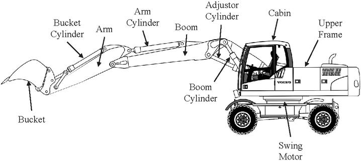
Figure 1 Volvo EWC210c wheeled excavator with the main components highlighted.
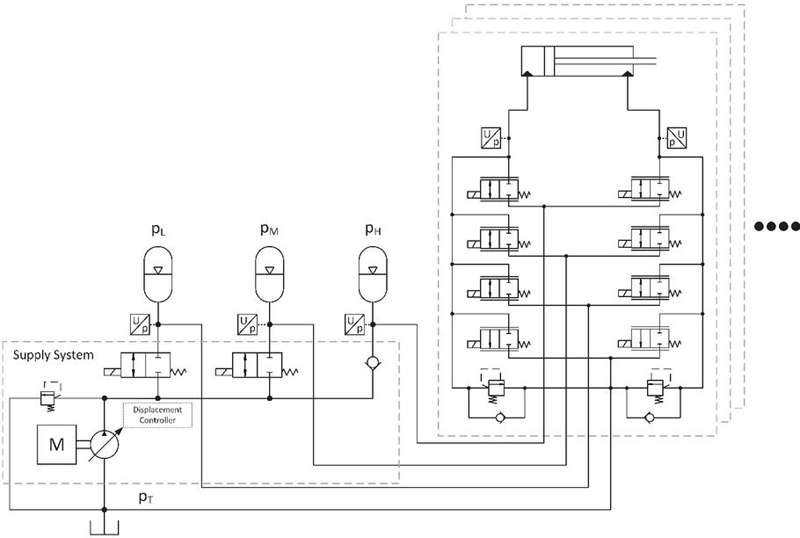
Figure 2 Simplified MPS showing main excavator functions.
A simplified hydraulic diagram of the new excavator MPS system is shown in Figure 2. The excavator is powered by a diesel engine operating a central variable displacement pump. The pump sends power to three piston type hydraulic accumulators at three pressure levels (, , ), each accumulator is fitted with a pressure sensor to control filling and emptying. The and accumulators have On/Off charge valves while the accumulator is fitted with a check valve. Each modified actuator in the excavator system is fitted with a valve manifold consisting of proportional 2/2 valves with four for piston side and four for the rod side responsible for selecting the pressure level and simultaneously adjusting their opening according to the required flow, supply pressure and load. The actuator inflow and outflow chambers are monitored with pressure sensors to measure the load force which is used to decide the current pressure level. In comparison, the original machine features a single variable displacement pump with a capacity of approximately 400 liters per minute, powering both the work hydraulics and the drive-train. Its valve system utilized hydro-mechanical load-sensing technology, employing closed-center downstream pressure-compensated valves. The schematic and description of the original machine can be found in a different study on the same excavator [39].
The modified MPS allows for multiple improvements over conventional throttling-based systems currently used in the industry. Firstly, the engine and pump are only required to supply mean power instead of peak power. The higher demand can be supplied by the accumulators which means the engine and pump can operate at a more efficient zone. Accumulators can store energy regenerated from boom lowering, swing deceleration and similar. Additionally, having multiple pressure levels to select from can minimize the pressure difference across the control valves and thus minimizing throttling losses specifically during simultaneous actuator operation. Finally, the suggested system also offers the practicality of only modifying the power supply system rather than changing the original actuators in comparison to, for example, multi-chamber cylinders.
To fully exploit the potential of the MPS system, an effective control algorithm is essential. The controller must efficiently select the appropriate pressure lines, while simultaneously optimizing the operation of the pump and diesel engine to minimize losses and reduce fuel consumption. In addition, precise regulation of the proportional valve openings is required to deliver the desired performance. Finally, the control strategy should provide system responsiveness and controllability comparable to or superior to the conventional approach.
2.2 Operating Principle
In each actuator port in the system there are four pressure supply lines to choose from for the inflow and outflow which are , , , . Multiple supply lines can be connected to one actuator port at the same time which is achieved through the proportional valves at each port. To achieve the required flow, there must be a minimum pressure difference across the control valve. The supply system recharges the depleted accumulators through the charge valves installed at each accumulator inlet, the pump’s displacement is controlled using a proportional electric solenoid. The control algorithm requires the knowledge of current load and line pressures which is done by measuring the cylinder port pressure to determine the load and accumulator pressure to detect supply pressure and hence the pressure difference across the current selected control valve.
Proportional control valves enable the supply of flow from multiple pressure levels simultaneously. This means that the chamber flow rate references for both the inflow and outflow sides can be distributed among different control valves, with each valve connected to a specific supply line.
The flow rate estimate is derived from the actuator’s velocity reference, which is based on the operator’s joystick signal. To achieve energy-efficient operation, the lowest available pressure lines are prioritized on the inflow side. In contrast, the highest-pressure lines are prioritized on the outflow side to maximize energy regeneration. For example, if the flow demand on the inflow side cannot be fully met by a single valve connected to the lowest pressure level, the system activates the next valve connected to the second-lowest pressure line to supply the remaining flow, and so on.
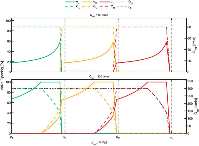
Figure 3 Flow rate references metered by individual valves as a function of the chamber pressure reference , are the corresponding valve opening and flow rate of each accumulator and are their pressure
To illustrate the valve manifold logic Figure 3 shows a simplified operation with an increasing chamber pressure reference on the inflow side under steady-state conditions. The increasing pressure reference represents increasing load force on the actuator. An example of the actuation logic of an actuator valve manifold using two reference flow rates is shown. In the upper graph, the flow rate reference is set at 80 and is metered at lower chamber pressure using the lowest supply line valve. As the pressure increases and approaches the supply pressure of the selected valve, the valve can no longer meter the required flow effectively. When the pressure difference becomes too small, the second-lowest pressure line is connected by opening the second valve. Simultaneously, the first valve closes to maintain flow control. The process is repeated selecting higher pressure supply lines as the chamber pressure is increased even more. The bottom graph shows a flow reference of 300 where the same operation principle can be noticed. The pressure lines are selected in ascending order until all the required reference flow is metered. It is also evident that the flow reference is metered by two valves with different supply pressures simultaneously. In addition to these features, the actuator controller contains several functions to prevent step-wise control signals, force peaks and other harmful phenomenon that comes as a result for switching between different pressure levels, this is discussed later in the controllers section. In summary, the actuator control first determines the load and supply pressures through pressure sensors while the flow reference is estimated through the velocity reference set by the operator. Second, the actuator controller operates the valves that:
1. Minimize the throttling losses and switching losses for the inflow and outflow sides.
2. Have high enough pressure to provide a differential across the valve to meter the flow and ensure correct direction of flow.
3. Prevent step wise control signals and disturbances.
4. Avoid the emptying of accumulators.
5. Reduce large pressure changes.
where the above control logic is applied for the inflow and outflow side in an identical fashion.
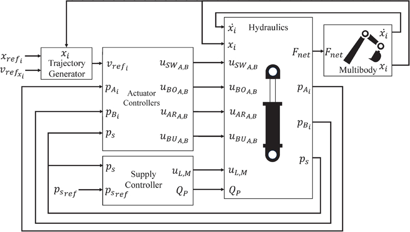
Figure 4 Simulation model of the MPS including control, hydraulics and multi-body dynamics
3 Multi-Pressure System Modeling
The MPS is modeled in MATLAB-Simulink environment where the excavator mechanics are modeled using Simscape multi-body dynamics while the hydraulic system is modeled in Simulink using non-linear physical modeling of components. The overall simulation model is shown in Figure 4. The trajectory generator represents the operator’s position command and is capable of generating preset trajectories. These trajectories were measured experimentally in previous research using the original machine’s load-sensing (LS) system. This allows the actuator movements in the simulation to closely match those measured from the original system, enabling meaningful comparisons. In the controller implementation the velocity reference is generated from the joystick commands through the operator. The trajectory generator does not receive velocity feedback from the system but is modeled corresponding to visual feedback of the operator giving correct velocity reference through the joystick [36].
The actuator controllers are responsible for generating the valve opening commands for each actuator’s inflow and outflow sides, where denotes each actuator: swing (SW), arm (AR), boom (BO), and bucket (BU) and A,B representing cylinder ports. In parallel, the supply controller uses the accumulators’ reference pressures to activate the pump flow rate and the charge valve openings , which are then used as inputs to the hydraulics model to start the charging of the accumulators. This model outputs the chamber pressures , , actuator net force , and the accumulators pressures which serve as inputs to both the actuator and supply controllers. The net forces produced by the hydraulic cylinders drive the movement of the excavator’s components in the multi-body dynamics model. It should be noted that the swing actuator is in reality a hydraulic motor, but mathematically it is modeled as a symmetric cylinder with piston area replaced with radian displacement and piston velocity with angular velocity. The dynamics model computes the positions and velocities of each actuator, which are used as feedback to the hydraulics model. The details of each model component and how all the values are calculated are provided in this section.
3.1 Multi-body Dynamic Excavator Model
The analysis of the excavator system requires complete modeling of component dynamics. This is done using the MATLAB Simscape toolbox which requires the definition of all kinematic relations, inertia, masses and other dynamic properties. The mechanical properties such as the masses and inertia are obtained directly from the manufacturer through their CAD models. Some assumptions were made due to the difficulty in obtaining certain data which includes:
• Friction is lumped into the actuator’s friction model.
• Rigid body assumption
These assumptions don’t have a noticeable effect on the results since they are small compared to actual forces generated by the hydraulic system. The Simpscape multi-body dynamics model provides a way to calculate the complex relations and equations of motion of the system. The model uses the input forces and torques and calculates the output position and speed of each actuator. Parameters used in the Simscape model are provided by the manufacturer ensuring accurate representation of geometry, mass properties, and inertia of each component.
3.2 Hydraulic System Mathematical Model
The hydraulic system simulation model consists of valves, cylinders, swing motor, accumulators and a pump. In the MPS there are several components that have the same modeling approach such as the cylinders, valves and accumulators. The next section provides the general modeling techniques that can be applied for all the similar components rather than detailing each individual part with specific abbreviations. For example, all accumulator pressures are modeled using the same equations and are referred to collectively as and similarly for the valves, all actuator cylinders and charge valves.
3.2.1 Hydraulic cylinders
The cylinder forces of the boom, arm and bucket are all modeled using the same principles. The actuator forces are summed to a net force that is connected to the mechanical system where the dynamics and kinematic relations calculations are done, the net force is:
| (1) |
where is the cylinder friction force represented using a Stribeck curve and is calculated from [35]:
| (2) |
such that is a coefficient to smooth the zero velocity crossing, , are the coulomb and static frictions, is the minimum friction velocity and is the viscous friction coefficient.
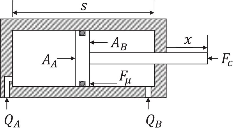
Figure 5 Schematic and parameters of the double-acting cylinder.
The cylinder force for any actuator can be calculated from:
| (3) |
where and are the piston and rod side areas of the respective cylinder shown in Figure 5. The chamber pressures and are calculated through build-up equations:
| (4) | |
| (5) |
where is the piston velocity calculated from the multi-body dynamics model, and are the fluid volumes and effective bulk modulus of each chamber respectively and is the net flow rate to the cylinder chambers which is the sum of flow rates from each supply line valve detailed in the control valves section. The volumes depend on the specific chamber where for chamber :
| (6) |
and for chamber :
| (7) |
where is the piston current stroke from the dynamics model, is the total stroke of the cylinder, is the dead volume at each chamber end and is the hose volume connected to each chamber. The bulk modulus and fluid volume are modeled in detail in order to study their effect during pressurization since the pressure levels in the chambers are changing repeatedly during operation. The chamber’s effective bulk modulus takes into consideration the oil and hose bulk moduli and is calculated from [40]:
| (8) |
where is the oil’s bulk modulus, is calculated from 6 and 7 and is the bulk modulus of the hose.
3.2.2 Control valves
The control valves are electro-hydraulic proportional bidirectional valves. The inflow and outflow edges of cylinder are connected to each pressure line using multiple control valves. The flow requirement of each edge is metered using one or more pressure levels as outlined in the previous sections. All valves are modeled in a similar fashion where the single flow rate through one valve can be defined using the modified square root equation [41] that has a non-infinite derivative when the pressure difference is close to zero. The flow rate for one valve can be calculated from:
| (9) |
where for the A chamber or for B chamber, and is the supply pressure from the accumulators described below, is the valve opening vector for all edge valves between zero to one, is a threshold pressure below which the flow is calculated using an empirical laminar flow formula and is the valve’s flow coefficient defined by the nominal flow rate and pressure :
| (10) |
The flow rate to one chamber is the summation of all four valves connected to its port. Additionally, the valve opening is limited by movement time and opening and closing delays and the valve dynamics are approximated with a first order transfer function. The valve opening for each actuator cylinder inlet and outlet port is decided by the actuator controllers outlined in the controllers section.
To ensure that the modeled performance closely matches the actual system, all proportional and charging valve parameters, including flow coefficients and response times, were taken directly from the manufacturers’ data-sheets.
3.2.3 Accumulators
The accumulator system is modeled using a hydraulic capacitance, which represents the supply lines connected to the accumulator through an orifice emulating the charge valves. The accumulator itself is simulated using a lossless adiabatic gas model. The buildup equation is used to calculate the supply line pressure:
| (11) |
is the fluid’s bulk modulus, is the accumulator total volume and is the total flow rate from the pump, valves and accumulator respectively. The pressure of accumulator is calculated from the adiabatic expansion formula:
| (12) |
where is the pre-charge pressure, is the volume of accumulators at precharge, is the adiabatic expansion coefficient and is the gas volume calculated from:
| (13) |
is calculated similarly to (9) where , the charge valve opening set to zero or one and is set to the charge valve’s coefficient. The charging of the accumulators is done by setting their respected valve openings to one and the charging is stopped by closing the charge valves (setting the value to zero). The accumulators charge logic is presented in the supply system controller section.
3.2.4 Hydraulic pump
The hydraulic variable displacement pump used in the system is not modeled in detail. The pump is mainly simulated as a simple flow source with no dynamics or limitation where the pump flow rate is considered as constant when flow is demanded by the accumulators through the supply controller. The pump model can be illustrated using:
| (14) |
where is the pump command through the supply system controller. A more detailed pump model was tested and simulated achieving identical performance. However, to keep this article short the details were excluded.
3.2.5 Power and energy
The input power of the valves is calculated from the valves flow and the accumulator pressures where the power consumed by the valves is:
| (15) |
The output power of the system is calculated through the actuator forces and velocity where:
| (16) |
and the energy input to the valves is a simple trapezoidal integration of the consumed power.
4 Controllers
There are two main controllers that are responsible for the MPS operation which are the supply and actuators controllers. The supply system control main responsibility is to keep the accumulators between a certain minimum and maximum pressure. The actuator controllers select the valve openings for each of the actuator’s (Swing – Boom – Arm – Bucket) inlet and outlet valves according to current conditions. This section presents the logic behind both controllers, their main functionalities and how they fulfill system requirements, minimize energy consumption and regenerate energy.
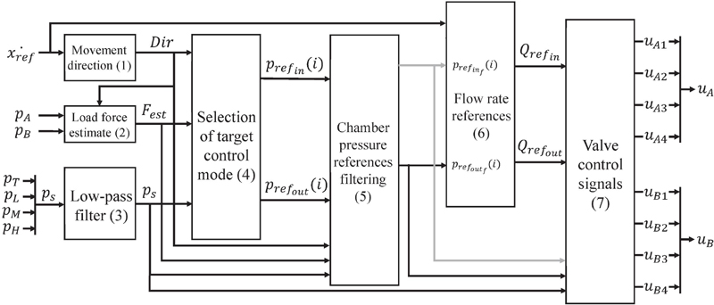
Figure 6 Block diagram of the actuators controller algorithm, the controller is similar for all actuators.
4.1 Actuator Controllers
The actuator controllers are responsible for selecting the valve openings for the inlet and outlet sides according to the reference velocity set by the trajectory generator “operator”, load force at the cylinder rod side and the supply pressure levels. This is done by adjusting the valve openings to meet all system operational requirements. Figure 6 shows the overall actuator controller algorithm where the calculation of the valve openings is done in seven steps explained in this section.
1. The first step is to determine the movement direction using the velocity reference which is needed to determine the inflow and outflow sides of the actuator using the following logic:
| (17) |
and in order to avoid repetitive initiation the logic includes hysteresis where is the reference velocity set by the operator, and are the velocity thresholds to start and stop motion, is the direction at the previous time step. The motion of the system is started only if the speed exceeds the set start speed in both directions and is stopped when the reference is lower than the set minimum speed. Controller inputs/outputs and system parameters for each side are assigned using the variable where for example the inflow-outflow areas are defined using:
| (18) |
this is done similarly for all other I/Os and parameters such as hydraulic capacitance, valve coefficients, inlet and outlet pressures, valve control input and control modes.
2. The actuator load force is estimated from the simulated low pass filtered chamber pressures , which is done to avoid repetitive mode switching using:
| (19) |
where , are calculated using:
| (20) |
and , are the corner frequency and damping coefficient of the second order low pass filter.
3. The third step contains the low pass filtering of the accumulators pressures which is done using (20) and the output is the supply pressure which is a vector containing all filtered pressure signals.
4. The movement direction, estimated filtered load force and filtered supply pressures are used to select the target mode that:
(a) Ensures large enough force to overcome the estimated load force.
(b) Minimizes power consumption.
(c) Prevents large changes in pressure levels
(d) Avoids emptying accumulators.
The control mode is the selection of pressure references for the piston and rod sides that can drive the actuator at the current conditions and accumulators levels. The control modes are selected based on a control matrix that has all the possible combinations of supply lines for the inflow and outflow sides which is:
| (21) |
(a) To ensure sufficiently large force, there must be an adequate pressure difference across the control valves for the inflow and outflow sides. Additionally, the pressure on both sides must remain between specified minimum and maximum limits. This process is carried out in two steps. First, the available reference pressure vectors for the inflow and outflow chambers are calculated using the control matrix and the following equation:
| (22) | ||
this equation assumes a symmetric pressure differential for both edges for simplicity. The inflow-side supply pressure is reduced by a margin, while the outflow-side supply pressure is increased by the same margin. Therefore, for the outflow:
| (23) |
This step outputs all the possible combinations of chamber pressure references from the decision matrix assuming equal pressure differential on both edges. These combinations satisfy the condition of overcoming the estimated load force but are not necessarily physically feasible. The second step checks these combinations for feasibility where candidates are evaluated making sure that they can be achieved hydraulically. The pressure references must be higher than a minimum defined value to avoid cavitation and the effects of bulk modulus variation on system dynamics at low pressure. Also, they must not exceed the maximum allowed system pressure . Additionally, for the outflow side the reference pressure must be higher than the accumulator pressure by a margin of to allow for metering. The matrix of all feasible combinations ensures that the mentioned requirements are fulfilled and is calculated using:
| (24) | ||
where is used to check If a selected accumulator’s pressure is too low where that line is considered as infeasible and is eliminated. can be checked using:
| (25) |
where are the accumulators’ minimum allowed pressures and is a hysteresis value to prevent chattering. This value stops the use of a specific accumulator when its pressure falls below the lower threshold. The accumulator is made available again once the pressure rises above the higher threshold and the hysteresis margin. The margin thus avoids rapid switching caused by pressure fluctuations around the charging threshold and eventually chattering.
(b) The feasible control candidates (non-feasible candidates are set to infinity) are screened using a cost function and the target modes for the inflow-outflow sides are selected using:
| (26) | ||
where the first line of the cost function represents the throttling losses of the control candidate.
(c) The second line penalizes large changes in pressure levels to minimize pressurization and switching losses
(d) Third line of the function penalizes using accumulators with lower pressure levels and encourages using full accumulators.
This is done using the weighing terms and and the supply pressure error calculated as:
| (27) |
where is the reference accumulators’ pressures.
The output of the cost function minimization is the control mode index which is used to select the target pressure references and from the candidates calculated in 22 and 23 for the next step.
5. If the selected reference pressure combination changes from the previous time step the controller commands a gradual increase of the pressure references. This is done to avoid force peaks and oscillations and outputs the filtered chamber pressure references.
6. The flow rate reference is mainly calculated using the actuator velocity reference and the chamber area. However, changing the pressure level also introduces flow requirement to pressurize the hydraulic capacitance of the actuator and hoses which is also taken into consideration when calculating the flow references for the inflow side and the outflow side .
7. The final step in the controller is to calculate the valve commands using supply pressures (3), chamber pressure references (5) and flow rate references in (6) where for:
• Inflow chamber:
The logic is to open a valve connected to the lowest possible pressure while at the same time maintaining a differential above the chamber pressure.
• Outflow chamber:
A valve is opened connected to the highest possible pressure while being lower than the outflow chamber pressure by the same minimum set pressure differential.
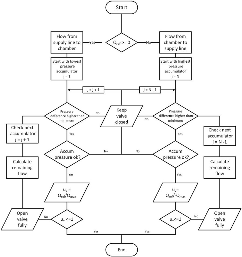
Figure 7 Flow chart of the valve actuation logic during operation.
If the opened valve is not capable of supplying the flow reference, next supply line is used to fulfill the flow requirement explained in the actuator control section. Figure 7 shows a flow chart for the valve actuation logic. First, the flow reference is sign checked to determine the flow direction then the accumulator is selected accordingly, if the pressure difference at the current accumulator is high enough and the accumulator’s pressure is not too low then the valve’s opening is set as:
| (28) |
If the valve is not fully opened this means that the flow reference is satisfied. However, if the opening is more than one this means that another valve needs to be open to complete the requirement which is done by setting the current valve to full opening and the new flow reference to the difference between current valve’s maximum flow and the original flow required:
| (29) |
the new flow reference is used with the next accumulator until the flow is metered completely. One exception is made to the highest pressure accumulator is that the pressure difference allowed is compared to allowing for reduced actuator performance but avoids stopping the actuators all together during extreme demand. The calculated valve commands from the actuator controller and are routed to the and ports of each cylinder using the direction of actuation where is:
| (30) |
where represent the swing, arm, boom and bucket actuators respectively and each actuator port commands is a vector for each single valve of the valve manifold. For example the command is:
| (31) |
The previous steps illustrate the main algorithm for the valve actuation. Although the MPS differs from Load-Sensing (LS) systems, certain functionalities were introduced to emulate some LS-like behaviors under high-demand conditions. Specifically, a velocity reference scaling mechanism is implemented to reduce actuator velocity during periods of prolonged high flow demand by the operator. In traditional LS systems, such behavior resembles the effect of flow saturation, where the pump reaches its volumetric capacity at a given engine speed and cannot maintain the required pressure differential across the valve. This results in slower actuator response due to limited available flow.
In contrast, the MPS system features accumulators that decouple the load dynamics from the supply, meaning that high flow demands can be temporarily met by discharging the accumulators. However, sustained high flow operation risks fully depleting the accumulators if not constrained. To address this, the actuator velocity is proportionally scaled down based on the total accumulator pressure error, which reflects the deviation of current pressures from their respective targets. This approach ensures that extended, high-energy operations result in a performance reduction rather than completely emptying the accumulator and risking the stopping of the actuators.
The accumulator pressure error is the sum of differences between the accumulators current pressure and their target where. The proportionality factor can be calculated from:
| (32) |
where and is set to 50 bar. The limited velocity reference is calculated using the gain where:
| (33) |
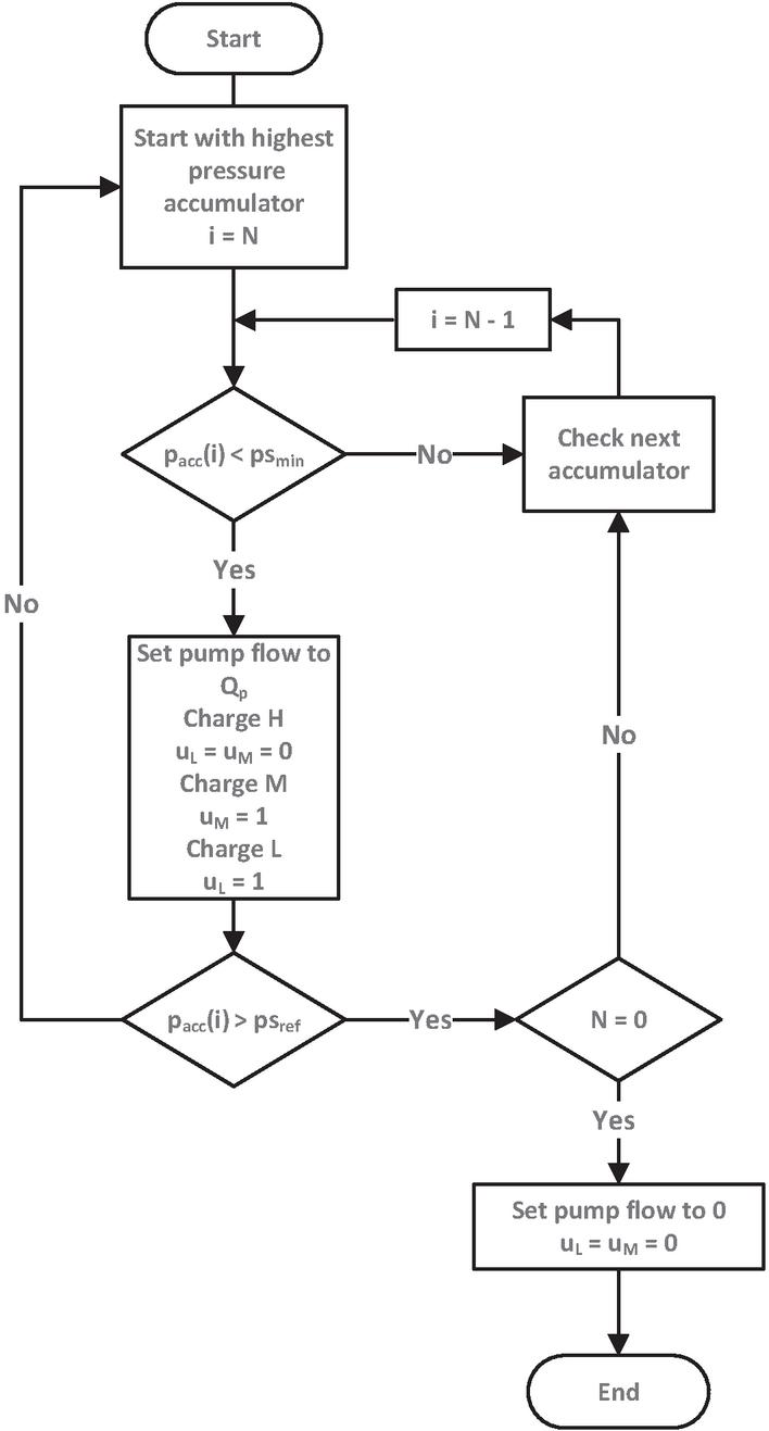
Figure 8 Flow chart of the supply system operation logic.
4.2 Supply System Controller
Figure 8 shows the control logic of the simplified supply system. It consists mainly of a diesel engine, variable displacement pump connected to an electronic control valve that adjusts the pump displacement, two On/Off charge valves and a check valve. The electronic flow control valve is responsible for setting the pumps flow according to which accumulator needs charging. The On/Off valves enable charging of the and accumulators and the highest pressure accumulator is charged when the pump pressure reaches the cracking pressure of the check valve and the low and medium charge valves are set to off. The decision to start charging an accumulator is taken when its pressure is lower than the reference pressure by a predefined value and the charging stops once the pressure has reached the reference. Priority is given to the higher pressures first meaning that the accumulators charge in the order of high, medium then low. After an accumulator is selected to charge its charge valve is open or for the high pressure both charge valves are closed.
The supply system controller and model are simplified in the simulation model. For example, the pump, diesel engine and valve dynamics are neglected. It is assumed that the pump is capable of supplying the demanded flow instantly and that the engine is capable of supplying the required power. Finally, the switching between the charge valve and check valves is the simple logic illustrated above. Although the supply controller and model are simplified in this work, similar results were reproduced using an advanced controller and supply system models. This is done as the focus is to highlight the capabilities of the MPS valve controllers and its energy saving potential.
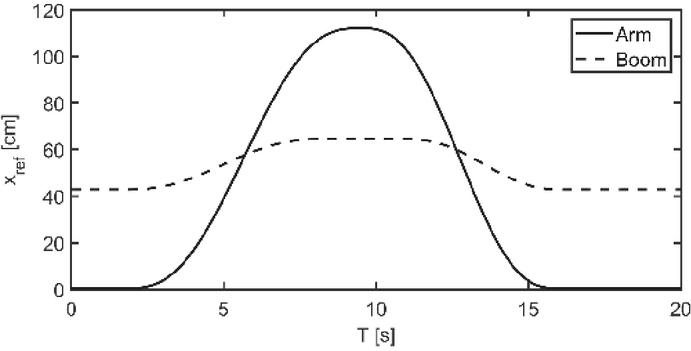
Figure 9 Reference trajectories generated by the operator model.
5 Simulation
5.1 Working Cycle
The simulated cycle shown in Figure 9 is a 20s air grading cycle from the JCMAS standard [42] where the boom and arm cylinders are extended and retracted simultaneously against the mechanism load representing leveling operation. Due to the complexity of modeling the machine-terrain interaction no load is introduced to the system apart from the component masses and inertia. This cycle gives an indication of the system operation during multiple actuators movement since the arm and boom are operated at the same time. It also provides insights on the accumulators performance since the actuators are operated at full speed demanding high flow rates.
Although the air grading cycle can be easily repeated it still has some limitations. For instance, it is not the best representative cycle in terms of quantifying the energy savings during real operation. Additionally, it can show unrealistic energy savings when compared to an LS-system which exhibits much higher compensation losses with no load applied. Also, the energy recovery mechanism can alter the system’s efficiency profile indicating higher savings than what can be actually realized in a more practical working cycle [43]. Nonetheless, with the limitations of the cycle acknowledged it can be understood that the energy savings are more indicative of the relative system improvement rather than projection to real-world savings.
The reference trajectories generated by the operator model shown in Figure 9 are generated using a proportional controller and a velocity feedforward term where the reference velocity can be calculated from:
| (34) |
where , are the controller gains, is the unmodified velocity reference and is the position reference.
Table 1 Volvo EW210c wheeled excavator main specifications
| Component | Value |
| Machine mass | 21160 kg |
| Engine power | 127 kW @1900 RPM |
| Engine torque | 730 Nm @1400 RPM |
| Pump Flow rate | 399 l/min |
| Maximum pressure | 360 bar |
| Accumulator pressures | [106 213 320] bar |
| Accumulator volumes | 15 l |
5.2 Simulation Results
The simulation is based on the mentioned 20-ton excavator (Volvo EW210C) where the parameters of the multi-pressure system are shown in Table 1. The simulation is run using the recorded cycle to illustrate the performance of valve and supply controllers under operating conditions. The energy consumption and losses of the system are also recorded to be compared to the original LS system whose measurements are available from previous research [39].
In order to measure the performance of the system several results must be taken into consideration. First, the system’s position and velocity should closely match that of the original system to make sure that similar work is done for a fair comparison. Then, the pressure levels of the accumulators and cylinder chambers must be within acceptable range to avoid pressure peaks, oscillations and depleted accumulators. Additionally, valve command signals for both chambers must be studied to ensure realistic operation. Finally, the energy losses in the system should be inspected to quantify the losses, where they occur and compare them to the LS-System.
5.2.1 Performance
Figures 10 and 11 show the simulation results for the two studied actuators of the excavator: Boom and Arm. The first two diagrams of the results show the position and velocity tracking performance. The velocity tracking also includes the limited velocity reference which is constrained by the pressure levels of the accumulators. The second diagram shows the pressures of: accumulators, chambers, chamber references generated by the controller and the dashed black line shows when the supply system is active and charging an accumulator. Finally, the bottom two diagrams show the openings of each control valve for each chamber. The colors in the bottom diagram match those of each pressure level.
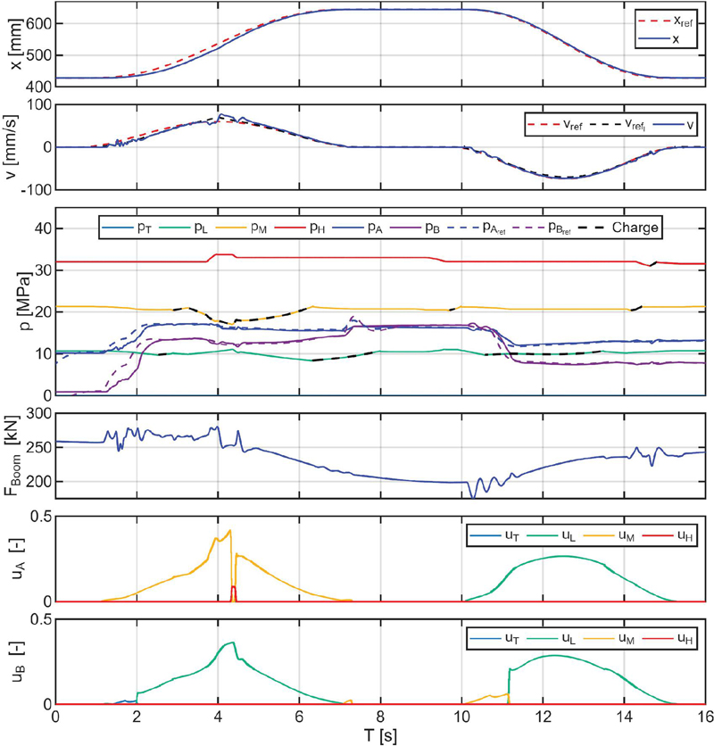
Figure 10 Boom actuator performance including position, velocity, accumulator and chamber pressure, actuator force and valve commands for A and B chambers.
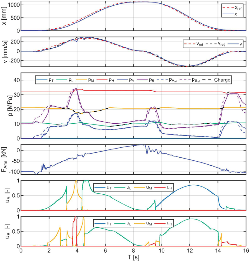
Figure 11 Arm actuator performance including position, velocity, accumulator and chamber pressure, actuator force and valve commands for A and B chambers.
The boom actuator tracking performance is good with some variations in velocity due to the operator model. Nonetheless, final position of the actuator matches the reference position well enough. Some small oscillations are noticed in the velocity response when the valves are switched between different pressure levels. The highest pressure level accumulator is not used during the boom operation where during extending motion chamber A is connected to and chamber B is connected to . Although this works for a duration of time, the medium pressure accumulator is discharged and the pressure difference is not enough to overcome the load pressure where chamber A connects momentarily to . As soon as the medium pressure accumulator is charged, the chamber pressures revert to their original targets. During extending motion both chambers connect to the low pressure accumulator. One benefit of the MPS is that energy can be recuperated by directing flow from the actuator chambers to an accumulator which can be seen in the low pressure accumulator at around 4 seconds where it’s pressure increases without using the supply system by directing flow from the actuator chambers to it.
Similar performance in terms of velocity and position tracking can be seen for the arm cylinder where the final required position is the same with some variations in velocity tracking which is attributed to the operator model. Additionally, the arm cylinder slowed down slightly (seen at 3–5 sec) which is attributed to saturating the A chamber input valves necessitating the opening of simultaneous valves. However, the arm cylinder controller exhibits different behavior to the boom cylinder where more switching between pressure levels can be noticed during extending and retracting due to higher variation on the magnitude of the load force. This can be clearly seen in the B chamber valve commands in the bottom diagram. During extending motion chamber B is connected to while A is connects to since the actuator is operating against over-running load resulting in energy recuperation. As the load pressure decreases in the B chamber, the pressure difference becomes too small and the controller has to switch to several times. During retraction motion chamber A connects to while B connects to since at the beginning of motion the over-running force is small. However as the piston extends further and the magnitude of over-running load force is increased, chamber A switches momentarily to and B is now connected to until the piston reaches its final position. The simulated cycle does not highlight the possibility of simultaneously opening of several pressure levels at the same time due to the overall low pressure of the load where the flow requirement can be fully metered using a single pressure level for almost the entire cycle, apart from a brief moment during the extension of the arm actuator where two valves can be seen open at the same time at around 5 seconds.
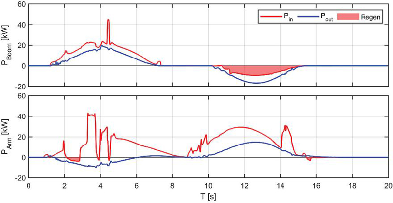
Figure 12 Input and output power of the boom and arm actuators.
5.2.2 Energy savings
The power consumption of both actuators during motion can be seen in Figure 12. The boom actuator consumes more energy at the moment where the medium pressure accumulator is discharged and chamber A connects to the high pressure accumulator leading to large pressure difference to the target and consequently larger throttling over the valve (can be seen after the 4 second mark) which could potentially be avoided if the supply system control reacts faster and charges the accumulators. On the other hand, the arm cylinder exhibits several power peaks and overall higher energy consumption compared to the boom cylinder. The initial increase in energy consumption, observed before 4 seconds, is due to chamber B connecting to the low-pressure accumulator. This results in high losses caused by flow throttling. The switch occurs as the over-running load force increases, leading to a drop in chamber pressure. As a result, the pressure difference is insufficient to utilize the medium-pressure accumulator. A second increase in energy consumption occurs during a pressure level change in both chambers, with chamber B shifting multiple times. Similar behavior is observed throughout the arm cylinder’s motion due to significant changes in load force, which cause multiple shifts between pressure levels.
Although the arm actuator exhibits high throttling losses when compared to the boom actuator, the overall energy consumption is low. The figure also highlights in red the duration were energy is regenerated in both actuators where the most significant regeneration occurs when the boom is lowered.
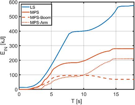
Figure 13 Energy consumption of the valves of MPS versus the original LS-System.
The difference in the energy needed to complete the grading cycle using the MPS and the original LS-system (measured experimentally in previous research) is illustrated in Figure 13. The energy needed for the MPS is which is lower when compared to of the LS-system. The reduction of energy in practice maybe slightly less due to the losses occurring during charging and discharging of accumulators as well as energy lost across the charge valves although their magnitude would be smaller compared to throttling losses in the actuator valves. The main contributors to the energy saving are reduced throttling losses and energy recuperation from the boom actuator when lowering the boom which can be seen between 10–15 seconds. As previously discussed in the section working cycle, these values are primarily indicative to the MPS potential rather than realistic savings, this is specially true since the energy recuperated can be significantly less under real-working conditions.
5.3 Control Challenges
The study highlighted several challenges to the control of MPS which needs further study. Firstly and most significantly, the controller decisions to switch between different accumulators highly depends on the pressure level of each accumulator at the decision time. For example, during the extending motion of the boom cylinder when was discharged forcing the switch to and consequently higher throttling losses. In addition to that, the future decision made by the algorithm may depend on the decisions made during an earlier phase which affects the pressure level in each accumulator. Therefore, It now would require different control decisions based on the new levels available. Also, the supply system operation greatly affects the MPS performance where a faster supply system may keep the pressure levels as steady as possible but still doesn’t guarantee an optimal overall system performance. In a similar note, the decision of when to charge the accumulators also complicates the control process. Although the presented controller offers some energy saving capabilities, it is difficult to define the interaction between the supply and actuators controller for optimum saving capabilities. For instance, even if the actuator controller is capable of optimizing its decisions internally the operation of the supply system could drastically alter those decisions by simply charging faster or slower. Similarly, the thresholds of starting to charge each accumulator (how much the pressure is allowed to drop) is currently defined heuristically but could be studied further to provide a more complete system performance. For example, they could be defined based on the energy available in the system or could be set at different thresholds for each accumulator based on the demanded flow. Despite these challenges, the presented controller was able to operate the MPS with good tracking performance.
6 Conclusion
A novel MPS capable of reducing the throttling losses typically abundant in state of the art commercial LS-systems is presented. It can improve the energy efficiency of hydraulic systems specifically during multiple actuator operation and more so in the work hydraulics. This paper presented the architecture and control algorithm of a novel system. The MPS valve and supply controllers were able to match the performance of original LS-system in terms of position and velocity commands while keeping the throttling losses lower than those of LS-system where an overall reduction in energy consumption was observed when comparing. Some undesirable phenomena were noted during system operation, these include the unwanted pressure level switching due to accumulator pressure changes as they are discharged which can be solved by using a faster supply system or using larger accumulator but doesn’t guarantee optimal operation. The energy saving capabilities were shown and the opportunities for energy recuperation is also discussed. Additionally, challenges to the control of the proposed MPS are presented, these included the operation of the supply system, how to define the charging thresholds for the accumulators and the interaction between the supply and actuators controllers. In future work, the MPS and its controllers are planned for testing on a 20-ton wheeled excavator. Research could also be conducted on the challenges in defining how an optimal MPS controller could look like, specifically in terms of defining the internal decisions between the supply system and actuator controls.
Acknowledgment
This research is funded through the Doctoral School Of Industry Innovation (DSII). It is a joint fund between Volvo CE and Tampere University, Finland.
Appendix
Nomenclature
: Piston side area of the respective cylinder
: Rod side area of the respective cylinder
: Inflow area of the actuator
: Outflow area of the actuator
: Viscous friction coefficient
: Fluid’s bulk modulus (for accumulator pressure build-up equation)
: Effective bulk modulus of chamber A or B
: Bulk modulus of the hose
: Oil’s bulk modulus
: Movement direction of the actuator
: Movement direction at the previous time step
: Margin by which inflow-side supply pressure is reduced and outflow-side supply pressure is increased
: Minimum set pressure differential across the control valve
: Pressure difference across the control valve
: Feasibility matrix
: Cylinder force
: Coulomb friction
: Estimated actuator load force
: Actuator net force
: Static friction
: Cylinder friction force, represented using a Stribeck curve
: Index denoting each actuator (swing, arm, boom, bucket)
: Cost function for selecting the target control mode
: Coefficient to smooth the zero velocity crossing (for friction model)
: Controller gain for velocity feedforward
: Proportionality factor for velocity scaling based on accumulator pressure error
: Proportional controller gain for position
: Valve’s flow coefficient
: Adiabatic expansion coefficient (for accumulator gas model)
: Control matrix containing all possible combinations of supply lines for inflow and outflow sides
: Chamber pressures for cylinder ports A and B
: Low-pass filtered chamber pressures for ports A and B
: Accumulator pressure
: High pressure level maintained by an integrated hydraulic accumulator
: Low pressure level maintained by an integrated hydraulic accumulator
: Medium pressure level maintained by an integrated hydraulic accumulator
: Maximum allowed system pressure
: Minimum defined pressure value to avoid cavitation and bulk modulus variation effects
: Minimum pressure to avoid cavitation
: Nominal pressure (for valve flow coefficient calculation)
: Pre-charge pressure (for accumulators)
: Chamber pressure reference
: Pressure references for inflow and outflow sides
: Supply pressure from accumulators (vector containing all filtered pressure signals)
: Reference accumulators’ pressures
: Accumulator pressure status, used to check if a selected accumulator’s pressure is too low
: Accumulators’ minimum allowed pressures (e.g., )
: Hysteresis value to prevent chattering (for accumulator pressure threshold)
: Supply pressure error ()
: Threshold pressure below which the valve flow is calculated using an empirical laminar flow formula
: Tank pressure
: Input power of the valves
: Output power of the system
: Flow into accumulator
: Flow rate corresponding to each accumulator
: Current valve’s maximum flow
: Nominal flow rate
: Pump flow rate
: Flow rate reference
: New flow reference, representing the difference between the current valve’s maximum flow and the original flow required
: Flow rate references for inflow and outflow sides
: Flow rate through one valve
: Net flow rate to the cylinder chambers A or B
: Total stroke of the cylinder
: Valve control signals for A and B chambers
: Valve opening commands for Boom actuator ports A and B
: Valve opening commands for Bucket actuator ports A and B
: Valve opening commands for Arm actuator ports A and B
: Calculated valve commands for inflow and outflow
: On/Off charge valve openings for pL and pM accumulators
: Pump command through the supply system controller
: Valve opening commands for Swing actuator ports A and B
: Valve opening vector for all edge valves (between zero and one)
: Valve opening for accumulator
: Valve opening corresponding to each accumulator (in valve manifold logic example)
: Accumulator total volume
: Fluid volumes of chamber A or B, dependent on piston stroke
: Gas volume (in accumulator)
: Hose volume connected to each chamber
: Dead volume at each chamber end for A and B
: Volume of accumulators at pre-charge
: Minimum friction velocity
: Velocity thresholds to start and stop motion
: Reference velocity set by the operator
: Limited velocity reference
: Unmodified velocity reference
: Weighing term for the cost function, penalizing the use of accumulators with lower pressure levels
: Weighing term for the cost function, penalizing large changes in pressure levels
: Piston current stroke from the dynamics model
: Position reference
: Piston velocity
: Velocity of each actuator
: Corner frequency of the second order low-pass filter
: Damping coefficient of the second order low-pass filter
Abbreviations
AR Arm actuator
BO Boom actuator
BU Bucket actuator
LS Load-Sensing hydraulic system
MPS Multi-Pressure System
SW Swing actuator
References
[1] Matti Linjama, Mikko Huova, Matti Pietola, Jyri Juhala, and Kalevi Huhtala. Hydraulic Hybrid Actuator: Theoretical Aspects And Solution Alternatives. In The Fourteenth Scandinavian International Conference on Fluid Power, Tampere, Finland, 2015.
[2] P. Hansson, Magnus Lindgren, M. Nordin, and O. Pettersson. A methodology for measuring the effects of transient loads on the fuel efficiency of agricultural tractors. Applied Engineering in Agriculture, 19, May 2003.
[3] M Lindgren and P. A Hansson. Effects of Transient Conditions on Exhaust Emissions from two Non-road Diesel Engines. Biosystems Engineering, 87(1):57–66, January 2004.
[4] Lonnie J Love. Estimating the Impact (Energy, Emissions and Economics) of the US Fluid Power Industry. Technical Report ORNL/TM-2011/14, 1061537, December 2012.
[5] Søren Ketelsen, Damiano Padovani, Torben Andersen, Morten Ebbesen, and Lasse Schmidt. Classification and Review of Pump-Controlled Differential Cylinder Drives. Energies, 12, April 2019.
[6] Joshua Zimmerman, Enrique Busquets, and Monika Ivantysynova. 40% Fuel Savings by Displacement Control Leads to Lower Working Temperatures – A Simulation Study and Measurements. In Proceedings of the 52nd National Conference on Fluid Power, Las Vegas, USA, March 2011.
[7] Joshua Zimmerman and Monika Ivantysynova. Hybrid Displacement Controlled Multi-Actuator Hydraulic Systems. In The Twelfth Scandinavian International Conference on Fluid Power, Tampere, Finland, 2011.
[8] M Eng Christopher Williamson. Power Optimization for Multi-Actuator Pump-Controlled Systems. In Proceedings of the 7 Th International Fluid Power Conference, Aachen, Germany, 2010.
[9] Milos Vukovic – Hydraulic Hybrid Systems for Excavators. PhD thesis, RWTH Aachen, Germany, 2017.
[10] P. Achten and J. Palmberg. What a difference a hole makes : The commercial value of the innas hydraulic transformer. In Proceedings of the 6th International Fluid Power Conference, Tampere, Finland, 1999.
[11] Kim Heybroek. Towards Resistance-free Hydraulics in Construction Machinery. In Proceedings of the 8 Th International Fluid Power Conference, Tampere, Finland, 2003.
[12] Georges Vael, Peter Achten, and Jeroen Potma. Cylinder Control with the Floating Cup Hydraulic Transformer. In Proceedings of the Eighth Scandinavian International Conference on Fluid Power, Tampere, Finland, May 2003.
[13] Peter Achten. Fundamentals of Hydraulic Transformers. In 14th International Fluid Power Conference, pages 796–815, Dresden, Germany, 2024. River Publishers.
[14] B Eriksson and J-O Palmberg. Individual metering fluid power systems: Challenges and opportunities. Proceedings of the Institution of Mechanical Engineers, Part I: Journal of Systems and Control Engineering, 225(2):196–211, March 2011.
[15] Mikko Huova, Matti Linjama, and Kalevi Huhtala. Energy Efficiency of Digital Hydraulic Valve Control Systems. SAE Technical Papers, 9, September 2013.
[16] Ruqi Ding, Bing Xu, Junhui Zhang, and Min Cheng. Bumpless mode switch of independent metering fluid power system for mobile machinery. Automation in Construction, 68:52–64, August 2016.
[17] Anders Hansen, Henrik Pedersen, Torben Andersen, and Lasse Wachmann. Investigation of Energy Saving Separate Meter-in Separate Meter-out Control Strategies. January 2011.
[18] Matti Linjama, Mikko Huova, Pontus Boström, Arto Laamanen, Lauri Siivonen, Lionel Morel, Marina Waldén, and Matti Vilenius. Design and Implementation of Energy Saving Digital Hydraulic Control System. The Tenth Scandinavian International Conference on Fluid Power, January 2011.
[19] Bin Yao and Song Liu. Energy-saving control of hydraulic systems with novel programmable valves. In Proceedings of the 4th World Congress on Intelligent Control and Automation (Cat. No.02EX527), volume 4, pages 3219–3223 vol.4, June 2002.
[20] Arne Jansson and Jan-Ove Palmberg. Separate Controls of Meter-in and Meter-out Orifices in Mobile Hyraulic Systems. SAE Technical Paper 901583, SAE International, Warrendale, PA, September 1990.
[21] M. Linjama, H.-P. Vihtanen, A. Sipola, and M. Vilenius. Secondary controlled multi-chamber hydraulic cylinder. In The 11th Scandinavian International Conference on Fluid Power SICFP’09, Linköping, Sweden, June 2-4 2009, Linköping, Sweden, 2009.
[22] Alessandro Dell’Amico, Marcus Carlsson, Erik Norlin, and Magnus Sethson. Investigation of a Digital Hydraulic Actuation System on an Excavator Arm. In 13th Scandinavian International Conference on Fluid Power, page 511, Sweden, 2013.
[23] Kim Heybroek and E. Norlin. Hydraulic Multi-Chamber Cylinders in Construction Machinery. In Hydraulikdagarna, Linköping, Sweden, 2015.
[24] Henri C Belan, Cristiano C Locateli, Birgitta Lantto, Petter Krus, and Victor J De. Digital Secondary Control Architecture for Aircraft Application. In The Seventh Workshop on Digital Fluid Power, Linz, Austria, 2015.
[25] Rico H. Hansen, Morten M. Kramer, and Enrique Vidal. Discrete Displacement Hydraulic Power Take-Off System for the Wavestar Wave Energy Converter. Energies, 6(8):4001–4044, 2013.
[26] NorrDigi is intelligent, energy-saving digital hydraulic solution. https://www.norrhydro.com/en/norrdigi-digital-hydraulic-solution, June 2024.
[27] Peter Dengler, Marcus Geimer, Heiko Baum, Gerhard Schuster, and Christoph Wessing. Efficiency Improvement of a Constant Pressure System using an Intermediate Pressure Line. In 8th International Fluid Power Conference, 26.-28. März 2012, Dresden, 2012.
[28] John H Lumkes John and Andruch John. Hydraulic Circuit for Reconfigurable and Efficient Fluid Power Systems. In The Twelfth Scandinavian International Conference on Fluid Power, Tampere, Finland, 2011.
[29] Milos Vukovic. STEAM: A Mobile Hydraulic System With Engine Integration. In ASME/BATH 2013 Symposium on Fluid Power & Motion ControlAt: Sarasota, Florida, USA, 2013.
[30] Miloš Vuković, H. Murrenhoff, and Roland Leifeld. STEAM – a hydraulic hybrid architecture for excavators. March 2016.
[31] Milos Vukovic and Hubertus Murrenhoff. Single Edge Meter Out Control for Mobile Machinery. In ASME/BATH 2014 Symposium on Fluid Power and Motion Control. American Society of Mechanical Engineers Digital Collection, 2014.
[32] Xiaofan Guo. Multi-Pressure Rail System Design with Variable Pressure Control Strategy. 2022.
[33] Xiaofan Guo, Jacob Lengacher, and Andrea Vacca. A Variable Pressure Multi-Pressure Rail System Design for Agricultural Applications. Energies, 15(17):6173, January 2022.
[34] Zihao Xu, Mateus Bertolin, Andrea Vacca, and Jan Nilsson. A Hydraulic Architecture Based on Multi-common Pressure Rail Principle Using Multi-chamber Cylinders for Excavators. In Liselott Ericson and Petter Krus, editors, Advancements in Fluid Power Technology: Sustainability, Electrification, and Digitalization, pages 339–356, Cham, 2025. Springer Nature Switzerland.
[35] Mikko Huova, Arttu Aalto, Matti Linjama, Kalevi Huhtala, Tapio Lantela, and Matti Pietola. Digital hydraulic multi-pressure actuator – the concept, simulation study and first experimental results. International Journal of Fluid Power, 2017.
[36] Mikko Huova and Matti Linjama. Energy efficient throttling control of a multi-pressure system using a genetic algorithm and model predictive control. Proceedings of the Institution of Mechanical Engineers, Part I: Journal of Systems and Control Engineering, 236(2):406–417, 2022.
[37] Mateus Bertolin and Andrea Vacca. A Parametric Study on Architectures Using Common-Pressure Rail Systems and Multi-Chamber Cylinders. In GFPS2022, Italy, 2022.
[38] Matti Linjama, Mikko Huova, Jyrki Tammisto, Mikko Heikkilä, Seppo Tikkanen, Jyrki Kajaste, Miika Paloniitty, and Matti Pietola. HYDRAULIC HYBRID WORKING MACHINES PROJECT – LESSONS LEARNED. May 2019.
[39] Miikka Ketonen and Matti Linjama. Digital Hydraulic IMV System in an Excavator – First Results. In The Sixteenth Scandinavian International Conference on Fluid Power, Tampere, Finland, May 2019.
[40] Matti Linjama and Mikko Huova. Model-based force and position tracking control of a multi-pressure hydraulic cylinder. 2018.
[41] Asko Ellman and Robert Piché. A Modified Orifice Flow Formula for Numerical Simulation of Fluid Power Systems, volume 3. November 1996.
[42] JCMAS – Earthmoving machinery – Energy consumption test method – Hydraulic excavator, 2010.
[43] Reno Filla. Representative Testing of Emissions and Fuel Consumption of Working Machines in Reality and Simulation. SAE paper 2012-01-1946, September 2012.
Biographies

Mohamed Allam received an MSc degree from Ain Shams University, Egypt, in 2020. He is currently a doctoral researcher at Tampere University, Tampere, Finland, pursuing a Ph.D. in Automation Science and Engineering. He works in the Innovative Hydraulics and Automation Lab, focusing on energy-efficient machines, hybrid technologies, and powertrain modelling and simulation.

Mikko Huova received a DSc degree from Tampere University of Technology, Finland, in 2015. His thesis focused on energy-efficient digital hydraulic systems. He continues work in this field as a postdoctoral researcher at TUT. His research interests include control design, modelling, simulation, and energy-efficient systems.

Kim Heybroek was born in Vastervik, Sweden, in 1981. He received the M.Sc. degree in mechanical engineering from Linköping University, Sweden, in 2006. In 2008, he joined Volvo Construction Equipment in Eskilstuna, where he works as a Research Engineer and Specialist in hydraulics. In 2017, he received the Ph.D. degree in hydraulics at the Department of Fluid Power and Mechatronic Systems (FluMeS) at LiU.
International Journal of Fluid Power, Vol. 27_2, 257–296
doi: 10.13052/ijfp1439-9776.2721
© 2026 River Publishers