Dynamic Analysis of an Adjustable Linkage Mechanism for a Low-Speed, High-Torque Hydraulic Motor

Jonatan Pozo-Palacios, Grey C. Boyce-Erickson, Justinus K. Hartoyo, Martin Herrera-Perez, John A. F. Voth and James D. Van de Ven^*

Department of Mechanical Engineering, University of Minnesota, Minneapolis, MN 55455, USA
E-mail: vandeven@umn.edu
*Corresponding Author

Received 19 March 2025; Accepted 20 November 2025

Abstract

Adjustment of hydraulic motor displacement plays a critical role in regulating hydraulic circuits across a wide range of applications. However, the absence of commercially available continuously variable low-speed high-torque (LSHT) motor architectures poses a challenge. To evaluate a potential solution, this paper presents the dynamic analysis of an adjustable low-speed high-torque motor, the variable displacement linkage motor, with an emphasis on understanding the dynamics at different operating conditions. The hydraulic motor studied consists of five phase-shifted cam-linkage mechanisms that can be dynamically adjusted to change the displacement within certain limits. The primary contribution of this paper is the mathematical modelling of the kinematics and dynamics of the adjustable linkage mechanism to explore the relative impact of the inertial, friction, and pressure-based forces. The results of the dynamic analysis reveal that inertial forces are higher when decreasing the displacement vs. increasing the displacement. Furthermore, at an operating pressure of $\mathrm{\Delta }$p $=$ 22 MPa, there is a notable 47.1% increase in actuation force when the settling time is reduced from 150 to 25 ms. Additional analyses cover the influence of inertial forces on actuator force at various operating pressures, and the adjustment actuator flow rate requirements associated with different adjustment times.

Keywords: Dynamic analysis, cam-linkage mechanism, low-speed high-torque, hydraulic motor.

Nomenclature

Variable Name	Description
$\overrightarrow{L_3},\overrightarrow{L_5},\overrightarrow{L_6}$ [m]	Coupler sides
$\overrightarrow{L_4}$ [m]	Rocker link
$\overrightarrow{P}$ [m]	Vector from the adj. ground pivot to TDC
$\overrightarrow{T}$ [m]	Vector from motor centre to TDC
${\theta }_{53}$ $[Rad]$	Angle between $\overrightarrow{{\mathrm{L}}_3}$ and $\overrightarrow{{\mathrm{L}}_5}$
${\theta }_{XX}$ $[Rad]$	Angle of vector $\overrightarrow{\mathrm{XX}}$. This applies to all vectors.
$\overrightarrow{L_7},\overrightarrow{L_9},\overrightarrow{L_{10}}$ $[Rad]$	Displacement adjustment link sides
$\overrightarrow{L_8}$ [m]	Vector from motor centre to $\overrightarrow{{\mathrm{L}}_7}$ pivot
$\overrightarrow{L_{11}}$ [m]	Displacement adjustment link II
$\overrightarrow{L_{12}},\overrightarrow{L_{13}},\overrightarrow{L_{16}}$ [m]	DAM ring side
$\overrightarrow{L_{14}}$ [m]	Linear actuator
$\overrightarrow{L_{15}}$ [m]	Vector from motor center to $\overrightarrow{{\mathrm{L}}_{14}}$ pivot
$l_{XX}$ [m]	Length of vector $\overrightarrow{\mathrm{XX}}.$ This applies to all vectors.
${\omega }_{xx}$ [rad/s]	Angular velocity of link ${\mathrm{l}}_{\mathrm{XX}}$
${\alpha }_{xx}$ [rad/s2]	Angular acceleration of link ${\mathrm{l}}_{\mathrm{XX}}$
$c(t)$	System response
$A_s$	Amplitude
${\omega }_n$ [Hz]	Natural frequency
Tf	Tolerance fraction
t [s]	time
$u(t)$	Unit step input
$T_s$ [s]	Settling time
$p_{cyl}$ [Pa]	Cylinder pressure
$V_{cyl}$ [m3]	Cylinder volume
$Q_{in}$ [m3/s]	Flow rate in
$Q_{out}$ [m3/s]	Flow rate out
$v_p$ [m/s]	Piston velocity
$A_p$ [m2]	Piston area
$C_d$	Discharge coefficient
$p_{in}$ [Pa]	Inlet pressure
$p_{out}$ [Pa]	Outlet pressure
$\overrightarrow{F_{12,y}}$ [N]	Vertical force exerted by the cylinder on the piston
$\overrightarrow{F_p}$ [N]	Fluid pressure force applied on piston
$\overrightarrow{F_{32}}$ [N]	Force exerted by the coupler on the piston
$\overrightarrow{F_{C3}}$ [N]	Force exerted by the cam on the coupler
$\overrightarrow{F_{43}}$ [N]	Force exerted by the rocker on the coupler
$\overrightarrow{F_{94}}$ [N]	Force exerted by DAM link I on rocker
$\overrightarrow{F_{19}}$ [N]	Force exerted by ground on the DAM link I
$\overrightarrow{F_{11,9}}$ [N]	Force exerted by DAM link I on the DAM link II
$\overrightarrow{F_{13,11}}$ [N]	Force exerted by DAM ring on DAM link II
$\overrightarrow{F_{14,13}}$ [N]	Force exerted by the linear actuator on the DAM ring
$\overrightarrow{F_{1,13}}$ [N]	Force exerted by ground on by DAM ring
$\overrightarrow{F_{1,14}}$ [N]	Force exerted by ground on the linear actuator
$\overrightarrow{F_{1C}}$ [N]	Force exerted by ground on the cam
$R_C$ [m]	Instantaneous cam radius
${\theta }_C$ [Rad]	Instantaneous cam angle
${\theta }_N$ [Rad]	Cam normal vector force angle
$m_2$ [kg]	Piston mass
$m_3,I_3$ [kg, kg.m2]	Coupler mass and inertia
$m_4,I_4$ [kg, kg.m2]	Rocker mass and inertia
$m_9,I_9$ [kg, kg.m2]	DAM link I mass and inertia
$m_{11},I_{11}$ [kg, kg.m2]	DAM link II mass and inertia
$m_{13},I_{13}$ [kg, kg.m2]	DAM ring mass and inertia
$m_{14}$, $I_{14}$ [kg, kg.m2]	Linear Actuator mass and inertia
CG	Center of gravity
$l_{3b},l_{3c},l_{3d}$ [m]	Coupler: Distances between joints and CG
${\theta }_{3b},{\theta }_{3c},{\theta }_{3d}$ [Rad]	Coupler: Angles of ${\mathrm{l}}_{3\mathrm{b}},{\mathrm{l}}_{3\mathrm{c}},{\mathrm{l}}_{3\mathrm{d}}$
$l_{43},l_{49}$ [m]	Rocker: Distances between joints and the CG
$l_{91},l_{94},l_{9,11}$ [m]	Disp. Adj. link I: Distances between joints and the CG
${\theta }_{91},{\theta }_{94},{\theta }_{9,11}$ [Rad]	Disp. Adj. link I: Angles of ${\mathrm{l}}_{91},{\mathrm{l}}_{94},{\mathrm{l}}_{9,11}$
$l_{11,9},l_{11,13}$ [m]	Disp. Adj. link II: distances between nodes and the CG
$l_{13,1},l_{13,11},l_{13,14}$ [m]	DAM Ring: Distances between joints and the CG
${\theta }_{13,1},{\theta }_{13,11},{\theta }_{13,14}$ [Rad]	DAM Ring: Angles of ${\mathrm{l}}_{13,1},{\mathrm{l}}_{13,11},{\mathrm{l}}_{13,14}$
$T_{DLI,1}$ [Nm]	Frictional torque between DAM link I and ground
$T_{DLI,DLII}$ [Nm]	Frictional torque between DAM links I and II
$T_{DR,1}[Nm]$	Frictional torque between DAM ring and ground
$T_{DR,11}[Nm]$	Frictional torque between DAM ring and DAM link II
$T_{LA,1}$ [Nm]	Frictional torque between actuator support and ground
$T_{LA,13}$ [Nm]	Frictional torque between actuator rod and DAM ring
$a_{CM}$ [m/s2]	Acceleration of link center of mass
$l_{CM}$ [m]	Distance from pin to link center of mass
$\theta$ [Rad]	Initial linkage angular position
$\delta$ [Rad]	Linkage change in angular position
$T_{\mu ,12}$ [Nm]	Frictional torque between links 1 and 2
$F$ [N]	Total joint force
$d_p$ [m]	Pin diameter
${\mu }_{dyn}$ [$-$]	Dynamic friction coefficient
$d_1$ [m]	Sealed surface diameter
$d_2$ [m]	Inside diameter
${\mu }_f$ [$-$]	Friction coefficient seal surfaces
$E$ [GPa]	Seal Young Modulus
$F_s$ [N]	O-ring frictional force
$F_{sx}$ [N]	Horizontal component of O-ring frictional force
$F_{sy}$ [N]	Vertical component of O-ring frictional force

1 Introduction

Hydraulic motors are important in fluid power systems, being responsible for generating rotational motion for a wide spectrum of machinery applications. In today’s market, there is a selection of fixed and discretely variable low-speed high-torque radial piston motors, alongside high-speed low-torque continuously variable displacement axial piston motors. Continuously variable displacement motors offer several advantages. Ivantysynova referred to variable displacement motors in hydrostatic transmissions as secondary controlled drives and highlighted their potential to enhance energy efficiency and reduce operational costs [1]. Biederman et al. explored hydraulic circuit architectures for aircraft applications finding that the integration of variable displacement hydraulic motors resulted in improved efficiency [2]. Hartoyo et al. demonstrated significant enhancements in fuel savings for a series hybrid architecture with a variable displacement linkage motor [3].

Continuously variable displacement low-speed, high-torque motors are currently not available. To address this limitation, a novel variable displacement linkage motor (VDLM) was developed. The VDLM consists of several linkage modules mounted on a single radial plane that drive a multilobed radial cam. A hydraulically operated displacement adjustment mechanism (DAM) is used to adjust the linkage modules, changing the stroke and the corresponding volumetric displacement. The development of the VDLM was influenced by the work of Wilhelm and Van de Ven with single-cylinder [4] and multi-cylinder variable displacement linkage pumps [5]. Fulbright et al. developed initial work for the design of the VDLM motor using model-driven design and optimization techniques [6]. Larson et al. experimentally tested the energy loss models of different subcomponents of a single-cylinder motor prototype [7]. Pozo-Palacios et al., proposed details of the kinematics formulation [8], and the methods for cam-linkage mechanism synthesis [9]. Lastly, Herrera et al. minimized torque ripple in the VDLM motor by optimizing piston trajectories and valve timing, achieving less than 5% ripple at corner conditions and under 12% across operating points, with simulation results validated experimentally [10].

Several studies have been conducted to assess the frequency range or bandwidth at which the variable displacement mechanism of pumps and motors can operate. A high-frequency range indicates a hydraulic motor´s capability to respond quickly to displacement adjustment commands, making it more suitable for applications requiring fast control response. Fast displacement adjustment is particularly important in mobile hydraulic systems, where energy recovery during deceleration, dynamic adaptation to load conditions, and rapid changes in operating states are critical to improving system efficiency and performance. Zeiger and Akers developed mathematical equations describing the swashplate torque for an axial piston pump [11]. Hydraulic and mechanical models were considered for the analysis. However, only steady-state conditions were analysed. Schoenau et al. performed the dynamic analysis of a variable displacement axial piston pump creating a mathematical model and validating the steady state and the dynamic response with experimental testing [12]. Manring and Mehta analysed the bandwidth frequency of pressure-controlled axial piston pumps, which usually have a bandwidth limit of 25 Hz, to understand why these operating limits exist [13]. Manring and Mehta created a comprehensive pump and valve model and found that reducing the swept volume of the control actuator and increasing the flow capacity of the control valve have the greatest impact on the bandwidth frequency that may be achieved.

Regarding the dynamic analysis of multibody systems, there are two techniques defined as inverse dynamics (kinetostatics) and forward dynamics. Inverse dynamics uses mechanism motion to calculate the forces required to produce that movement. In contrast, forward dynamics uses joint forces and torques to calculate motion using numerical integration. Forward dynamics is extensively studied by Nikravesh [14], while the inverse method is extensively studied by Norton [15] for its application to linkage mechanisms. Inverse dynamics has been previously employed in the analysis of variable displacement linkage pumps and motors at fixed displacement settings. This approach has been used to compute parameters such as the total output torque, torque ripple, and mechanical efficiency [6, 7, 16].

No previous research work has addressed the modelling of the adjustment dynamics of a low-speed high-torque hydraulic motor, nor has there been an evaluation of its performance at different operating conditions. As a result, this paper aims to fill these gaps by modelling, experimentally testing, and analysing the performance of the VDLM at different operating pressures, shaft speeds, and displacement adjustment times. The research work is organized as follows: first, a general description of the variable displacement linkage motor architecture is presented. Next, the vector loop representations of the linkage mechanisms are presented along with the equations of motion. Subsequently, the fundamental models for the cylinder pressure dynamics are presented. Then, the dynamic models of the linkage mechanisms are presented along with the models used to calculate frictional forces and torques. These models are then applied to analyse a hydraulic motor prototype. Finally, the model development results and the experimental validation of the adjustment mechanism are discussed, and conclusions are made.

2 Methods

2.1 Main Linkage Mechanism and Displacement Adjustment Mechanism Description

The variable displacement linkage motors consist of multiple adjustable linkage mechanisms mounted on a single radial plane where an internal or external drive cam is also located, see Figure 1. When the machine is in operation, the pressurized hydraulic fluid pushes the piston connected to the coupler which in turn pushes the cam through the roller follower. The piston, coupler, rocker, and roller follower are always moving when the motor is rotating. The adjustable ground pivot position defines the fractional displacement of the motor/pump, which is calculated as a percentage of the maximum volumetric displacement. Figure 1 uses two colours to differentiate the displacement adjustment mechanism from the main linkage mechanism. The movement of the linear actuator causes the displacement adjustment links to move. This movement, in turn, adjusts the position of the adjustable ground pivot and changes the fractional displacement. The speed at which the displacement changes can be increased or decreased depending on the linear actuator speed. Although Figure 1 shows only one main linkage mechanism, several main linkage modules can be connected to the displacement adjustment mechanism, increasing motor displacement, and reducing output torque ripple.

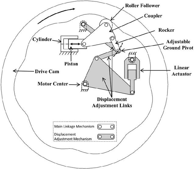
Figure 1 Components of main linkage mechanism and displacement adjustment mechanism.

2.2 Mechanism Kinematics

The kinematic and kinetic analyses are conducted by formulating and solving vector loop equations using the complex number method. This method is well known and has been extensively applied in the literature to analyse different mechanism topologies [15, 17]. Figure 2(a) shows the vector loop representation of the main linkage mechanism, and Figure 2(b) shows the vector loop representation of the displacement adjustment mechanism used for the dynamic analysis. The rocker is represented by the vector$\overrightarrow{{\mathit{L}}_{\mathbf{4}}}$, the coupler is represented by vectors $\overrightarrow{{\mathit{L}}_{\mathbf{3}}}$, $\overrightarrow{{\mathit{L}}_{\mathbf{5}}}$, $\overrightarrow{{\mathit{L}}_{\mathbf{6}}}$, the piston stroke is represented by the vector $\overrightarrow{\mathit{S}}$ (analysed with the piston traveling in the horizontal direction), and the position of the top dead centre (TDC) is defined by the vector $\overrightarrow{\mathit{T}}$, which is also defined by the vector $\overrightarrow{\mathit{P}}$, measured with respect to the adjustable ground pivot. The distance between the displacement adjustment pivot and the centre of the motor is represented by the vector $\overrightarrow{{\mathit{L}}_{\mathbf{8}}}$, and the link that changes the position of the adjustable ground pivot is represented by the vector $\overrightarrow{{\mathit{L}}_{\mathbf{7}}}$. Figure 2(b) shows the angle ${\mathit{\theta }}_{\mathbf{7}}$, which only changes when the displacement is adjusted, and the angle ${\mathit{\theta }}_{\mathbf{8}}$, which is constant for every motor design. In the same figure, the vectors $\overrightarrow{{\mathit{L}}_{\mathbf{7}}}$, $\overrightarrow{{\mathit{L}}_{\mathbf{9}}}$ and $\overrightarrow{{\mathit{L}}_{\mathbf{10}}}$ form ternary link that connects the rocker of the main linkage mechanism with the displacement mechanism. The vectors $\overrightarrow{{\mathit{L}}_{\mathbf{12}}}$, $\overrightarrow{{\mathit{L}}_{\mathbf{13}}}$ and $\overrightarrow{{\mathit{L}}_{\mathbf{16}}}$ represent a ternary link, also known as the displacement adjustment (DAM) ring, which rotates around the motor centre. The vector $\overrightarrow{{\mathit{L}}_{\mathbf{11}}}$ connects the DAM ring to the ternary link formed by $\overrightarrow{{\mathit{L}}_{\mathbf{7}}}$, $\overrightarrow{{\mathit{L}}_{\mathbf{9}}}$ and $\overrightarrow{{\mathit{L}}_{\mathbf{10}}}$. When the displacement is adjusted, the DAM ring rotates and changes the position of the adjustable ground pivot. Vector $\overrightarrow{{\mathit{L}}_{\mathbf{14}}}$ represents the linear actuator and therefore its magnitude and angle with respect to the ground pivot can change when the displacement is adjusted.

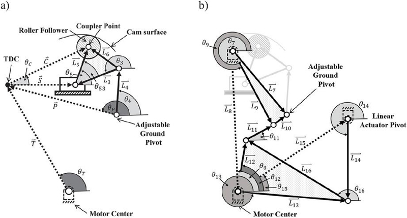
Figure 2 Vector loop representation of linkage mechanisms (a) main linkage mechanism and (b) displacement adjustment mechanism.

Main Linkage Mechanism Kinematics

The kinematics of the main linkage mechanism are described in reference [8]. The vector loop equations used for variable displacement analysis are presented below:

$$l_8{e}^{i{\theta }_8}+l_7{e}^{i{\theta }_7}+l_4{e}^{i{\theta }_4}+l_3{e}^{i{\theta }_3}-s_p=\stackrel{\rightharpoonup }{T}$$	(1)
$$s_p+l_5{e}^{i{\theta }_5}=\stackrel{\rightharpoonup }{C}$$	(2)

where ${\mathit{s}}_{\mathit{p}}$ is the piston stroke, lowercase $\mathit{l}$ represents the magnitude of the vectors and $\mathit{\theta }$ represents the vector angle. The rocker and coupler velocity and accelerations are calculated by numerical differentiation of ${\mathit{\theta }}_{\mathbf{3}}$ and ${\mathit{\theta }}_{\mathbf{4}}$.

Displacement Adjustment Mechanism Kinematics

The displacement adjustment mechanism can be divided into two sub-mechanisms. The first mechanism shown in Figure 2(b) is a rocker-slider consisting of the ternary link $\overrightarrow{{\mathit{L}}_{\mathbf{12}}}$-$\overrightarrow{{\mathit{L}}_{\mathbf{13}}}$-$\overrightarrow{{\mathit{L}}_{\mathbf{16}}}$, the adjustable link $\overrightarrow{{\mathit{L}}_{\mathbf{14}}}$, and the ground link $\overrightarrow{{\mathit{L}}_{\mathbf{15}}}$. The other mechanism is a four-bar consisting of the ternary link $\overrightarrow{{\mathit{L}}_{\mathbf{7}}}$-$\overrightarrow{{\mathit{L}}_{\mathbf{9}}}$-$\overrightarrow{{\mathit{L}}_{\mathbf{10}}}$ and the links $\overrightarrow{{\mathit{L}}_{\mathbf{8}}}$, $\overrightarrow{{\mathit{L}}_{\mathbf{11}}}$ and $\overrightarrow{{\mathit{L}}_{\mathbf{12}}}$.

The position equations for the slider rocker mechanism are presented below assuming that the angle ${\mathit{\theta }}_{\mathbf{15}}$ and all the linkage lengths are known.

$${\theta }_{{13}_{1,2}}=2ta{n}^{-1}\left(\frac{-B\pm \sqrt{B^2-4AC}}{2A}\right)$$

(3)

where A, B, and C are calculated with the following equations:

$$A=-\left[\frac{l_{14}^{}{}_{}{}^2-l_{13}^2-l_{15}^{}{}_{}{}^{2}co{s}^2({\theta }_{15})-l_{15}^{}{}_{}{}^{2}si{n}^2({\theta }_{15})}{2l_{13}}\right]+l_{15}cos({\theta }_{15})$$

$$B=-2l_{15}sin(l_{15})$$

$$C=-\left[\frac{l_{14}^{}{}_{}{}^2-l_{13}^2-l_{15}^{}{}_{}{}^{2}co{s}^2({\theta }_{15})-l_{15}^{}{}_{}{}^{2}si{n}^2({\theta }_{15})}{2l_{13}}\right]-l_{15}cos({\theta }_{15})$$

The angle ${\mathit{\theta }}_{\mathbf{14}}$ is calculated with the following equation:

$${\theta }_{14}=co{s}^{-1}\left[\frac{l_{11}cos({\theta }_{11})-l_{13}cos({\theta }_{15})}{l_{14}}\right]$$

(4)

The velocity equations for ${\mathit{\omega }}_{\mathbf{13}}$ and ${\mathit{\omega }}_{\mathbf{14}}$ can be obtained by deriving the Equations (3) and (4) with respect to time. A second derivative with respect to time of Equations (3) and (4) is used to calculate the acceleration equations for ${\mathit{\alpha }}_{\mathbf{13}}$ and ${\mathit{\alpha }}_{\mathbf{14}}$.

The position equations for the four-bar mechanism shown in Figure 2(b) are calculated with the following equations:

$${\theta }_{9_{1,2}}=2ta{n}^{-1}\left(\frac{-B_2\pm \sqrt{B_2^2-4A_2{C}_2}}{2A_2}\right)$$

(5)

where ${\text{A}}_2,{\text{B}}_2$, and ${\text{C}}_2$ are calculated with the following equations:

$$C_1=l_{8}cos({\theta }_8)-l_{12}cos({\theta }_{12})cos({\theta }_{15})$$
$$C_2=l_{8}sin({\theta }_8)-l_{12}sin({\theta }_{12})$$
$$C_3=\frac{l_{11}^{}{}_{}{}^2-l_{19}^{}{}_{}{}^2-C_1^{}{}_{}{}^2-C_2^{}{}_{}{}^2}{2l_9}$$
$$A_2=C_1+C_3$$
$$B_2=-2C_2$$
$$C_2=C_3-C_1$$
$${\theta }_{11}=co{s}^{-1}\left[\frac{l_{8}cos({\theta }_8)+l_{9}cos({\theta }_9)-l_{12}cos({\theta }_{12})}{l_{11}}\right]$$	(6)

The velocity equations ${\mathit{\omega }}_{\mathbf{9}}$ and ${\mathit{\omega }}_{\mathbf{11}}$ can be obtained by deriving Equations (5) and (6) with respect to time. A second derivative of Equations (5) and (6) with respect to time is used to calculate the acceleration equations for ${\mathit{\alpha }}_{\mathbf{9}}$ and ${\mathit{\alpha }}_{\mathbf{11}}$.

Linear Actuator Kinematics

To perform the inverse kinematics analysis of the linkage mechanism, it is necessary to define the position of the linear actuator during dynamic displacement adjustment. This is done by assuming that the linkage mechanism is represented by a second-order system with a fictitious natural frequency ${\mathit{\omega }}_{\mathit{n}}$ and critical damping $(\zeta =1)$. The system response to a step input in the time domain is given by:

$$c(t)=A_s[1-e^{-{\omega }_{n}t}(1+{\omega }_{n}t)]u(t)$$

(7)

where $\mathit{c}(\mathit{t})$ represents the system response, ${\mathit{A}}_{\mathit{s}}$ the amplitude, which in this case is the desired linear actuator stroke, u(t) is the unit step input function, and t is the time in seconds. The relationship between ${\mathit{\omega }}_{\mathit{n}}$, the settling time ${\mathit{T}}_{\mathit{s}}$, and the tolerance fraction $\mathit{t}\mathit{f}$ is given by:

$$tf=e^{-{\omega }_n{T}_s}(1+{\omega }_n{T}_s)$$

(8)

A tolerance fraction of $tf=0.02$, which is commonly used in control applications is considered. Defining a new variable $\mathit{x}={\mathit{\omega }}_{\mathit{n}}{\mathit{T}}_{\mathit{s}}$, Equation (8) becomes:

$$0.02=e^{-x}(1+x)$$

(9)

Equation (9) can be numerically solved to determine the relationship between ${\mathit{\omega }}_{\mathit{n}}$ and ${\mathit{T}}_{\mathit{s}}$:

$$T_s\approx \frac{5.8339}{{\omega }_n}$$

(10)

The velocity and acceleration of the linear actuator are obtained by taking the first and second derivatives of Equation (10) with respect to time.

Acceleration at the Link Centre of Mass

The acceleration at the centre of mass of each link is calculated with the following equation:

$$a_{CM}=l_{CM}(-{\omega }^2+i\alpha )e^{i(\theta +\delta )}$$

(11)

where ${\mathit{l}}_{\mathit{C}\mathit{M}}$ is the distance to the center of mass measured from one of the joints, $\mathit{\omega }$ is the link angular velocity, $\mathit{\alpha }$ is the link angular acceleration, $\mathit{\theta }$ is the initial link angle and $\mathit{\delta }$ is the link change in angle measured with respect to the initial position. This equation has real and imaginary terms, which correspond to the horizontal and vertical acceleration components. Additional information related to the acceleration analysis can be found in reference [18].

2.3 Cylinder Pressure Dynamics

To calculate the force applied to the piston, the cylinder pressure dynamics are solved with the following equation:

$$\frac{d{P}_{cyl}}{dt}=\frac{{\beta }_{eff}}{V_{cyl}}(Q_{in}-Q_{out}-v_p{A}_p)$$

(12)

where ${\mathit{Q}}_{\mathit{i}\mathit{n}}$ and ${\mathit{Q}}_{\mathit{o}\mathit{u}\mathit{t}}$ are the flow rates into and out of the cylinder, ${\mathit{\beta }}_{\mathit{e}\mathit{f}\mathit{f}}$ is the effective bulk modulus, ${\mathit{V}}_{\mathit{c}\mathit{y}\mathit{l}}$ is the cylinder volume and ${\mathit{v}}_{\mathit{p}}$ is the piston velocity. The effective bulk modulus is calculated using the equation proposed by Cho et al., which considers the variation of the bulk modulus as a function of cylinder pressure [19]. The flow rate in and out of the cylinder is calculated with the following expressions based on the orifice equation:

$Q_{in}$	$=C_d{A}_{in}\sqrt{{\displaystyle \frac{2}{\rho }}|P_{in}-P_{cyl}|}sgn(P_{in}-P_{cyl})$	(13)
$Q_{out}$	$=C_d{A}_{out}\sqrt{{\displaystyle \frac{2}{\rho }}|P_{cyl}-P_{out}|}sgn(P_{cyl}-P_{out})$	(14)

where ${\mathit{C}}_{\mathit{d}}$ is the discharge coefficient that can be estimated to be approximately 0.6 for a wide range of operating conditions [20], ${\mathit{P}}_{\mathit{i}\mathit{n}}$ is the inlet pressure, ${\mathit{P}}_{\mathit{o}\mathit{u}\mathit{t}}$ is the outlet pressure, $\mathit{\rho }$ is the fluid density and the valve areas are denoted by ${\mathit{A}}_{\mathit{i}\mathit{n}}$ and ${\mathit{A}}_{\mathit{o}\mathit{u}\mathit{t}}$. A spool valve positioned by a cam controls the flow in and out of the cylinder by adjusting the valve areas. The cam profile is defined using 5th-order polynomials to ensure continuous position, velocity, and acceleration of the spool valve. The inlet and outlet valve area profiles, ${\mathit{A}}_{\mathit{i}\mathit{n}}$ and ${\mathit{A}}_{\mathit{o}\mathit{u}\mathit{t}}$, were constructed using four polynomial segments for each valve. These segments include two ramps for the opening and closing transitions and two dwells representing the fully open and fully closed states. This piecewise formulation ensures smooth valve motion and accurate flow control throughout the cycle. The valve timing was optimized for several operating conditions, as detailed in reference [10], with the objective of minimizing torque ripple.

2.4 Dynamic Model of Linkage Mechanism

For the dynamic analysis, force and moment balances are performed on the main linkage mechanism and the displacement adjustment mechanism. Subsequently, within this section, an explanation of the frictional forces and torques is presented.

Force and Moment Balances

Figure 3 shows exploded views of the links, along with free-body diagrams for each component. The figure shows the forces acting on each element, along with dimensions, mass, and inertia properties.

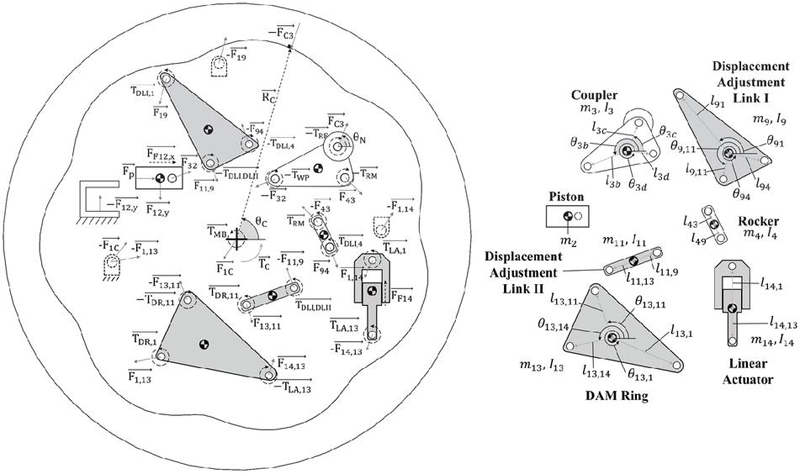
Figure 3 Exploded view and dimensions of linkage mechanisms.

The equations listed below are used for the full force balance. The nomenclature section includes the name and the description of every term. Moreover, all the frictional terms are displayed in bold:

Piston:

$$F_{32x}+F_p\pm {\mathit{F}}_{\mathit{F}\mathbf{12}\mathit{x}}=m_2{a}_{2x}$$	(15)
$$F_{12y}+F_{32y}=0$$	(16)

Coupler Link:

$-F_{32x}+F_{C3}cos({\theta }_N)+F_{43x}=m_3{a}_{3x}$	(17)
$-F_{32y}+F_{C3}sin({\theta }_N)+F_{43y}=m_3{a}_{3y}$	(18)
$-F_{32y}{l}_{3b}cos({\theta }_3+{\theta }_{3b})+F_{32x}{l}_{3b}sin({\theta }_3+{\theta }_{3b})+F_{c3}sin({\theta }_N)l_{3c}cos({\theta }_3$
$+{\theta }_{3c})-F{}_{c3}cos({\theta }_N)l{}_{3c}sin({\theta }_3+{\theta }_{3c})+F{}_{43y}l{}_{3d}cos({\theta }_3+{\theta }_{3d})$
$-F_{43x}{l}_{3d}sin({\theta }_3+{\theta }_{3d})-{\mathit{T}}_{\mathit{W}\mathit{P}}+{\mathit{T}}_{\mathit{R}\mathit{F}}+{\mathit{T}}_{\mathit{R}\mathit{M}}=I_3{\alpha }_3$	(19)

Rocker Link:

$-F_{43x}+F_{94x}=m_4{a}_{4x}$	(20)
$-F_{43y}+F_{94y}=m_4{a}_{4y}$	(21)
$-l_{43}cos({\theta }_4)F_{43y}+l_{43}sin({\theta }_4)F_{43x}-l_{49}cos({\theta }_4)F_{94y}+l_{49}sin({\theta }_4)F_{94x}$
$+{\mathit{T}}_{\mathit{D}\mathit{L}\mathit{I},\mathbf{4}}-{\mathit{T}}_{\mathit{R}\mathit{M}}=I_4{\alpha }_4$	(22)

Drive Cam:

$-F_{C3}cos({\theta }_N)+F_{1Cx}=0$	(23)
$-F_{C3}sin({\theta }_N)+F_{1Cy}=0$	(24)
$F_{C3}[R_{C}sin({\theta }_C)cos({\theta }_N)-R_{C}cos({\theta }_C)sin({\theta }_N)]$
$+T_C+{\mathit{T}}_{\mathit{M}\mathit{B}}=0$	(25)

Displacement Adjustment Link I:

$-F_{94x}+F_{11,9x}+F_{19x}=m_9{a}_{9x}$	(26)
$-F_{94y}+F_{11,9y}+F_{19y}=m_9{a}_{9y}$	(27)
$-F_{11,9x}{l}_{9,11}sin({\theta }_9+{\theta }_{9,11})+F_{11,9y}{l}_{9,11}cos({\theta }_9+{\theta }_{9,11})$
$+F_{94x}{l}_{94}sin({\theta }_9+{\theta }_{94})-F_{9,4y}{l}_{94}cos({\theta }_9+{\theta }_{94})$
$-F_{19x}{l}_{91}sin({\theta }_9+{\theta }_{91})+F_{19y}{l}_{91}cos({\theta }_9+{\theta }_{91})$
$+{\mathit{T}}_{\mathit{D}\mathit{L}\mathit{I},\mathbf{1}}-{\mathit{T}}_{\mathit{D}\mathit{L}\mathit{I},\mathit{D}\mathit{L}\mathit{I}\mathit{I}}-{\mathit{T}}_{\mathit{D}\mathit{L}\mathit{I},\mathbf{4}}=I_9{\alpha }_9$	(28)

Displacement Adjustment Link II:

$-F_{11,9x}+F_{13,11x}=m_{11}{a}_{11x}$	(29)
$-F_{11,9y}+F_{13,11y}=m_{11}{a}_{11y}$	(30)
$-F_{11,9y}{l}_{11,9}cos({\theta }_{11})+F_{11,9x}{l}_{11,9}sin({\theta }_{11})+F_{13,11y}{l}_{11,13}cos({\theta }_{11})$
$-F_{13,11x}{l}_{11,13}sin({\theta }_{11})+{\mathit{T}}_{\mathit{D}\mathit{L}\mathit{I},\mathit{D}\mathit{L}\mathit{I}\mathit{I}}+{\mathit{T}}_{\mathit{D}\mathit{R},\mathbf{11}}=I_{11}{\alpha }_{11}$	(31)

Displacement Adjustment Ring:

$F_{14,13x}-F_{13,11x}+F_{1,13x}=m_{13}{a}_{13x}$	(32)
$F_{14,13y}-F_{13,11y}+F_{1,13y}=m_{13}{a}_{13y}$	(33)
$-F_{14,13x}{l}_{13,14}sin({\theta }_{13}+{\theta }_{13,14})+F_{14,13y}{l}_{13,14}cos({\theta }_{13}+{\theta }_{13,14})$
$+F_{13,11x}{l}_{13,11}sin({\theta }_{13}+{\theta }_{13,11})-F_{13,11y}{l}_{13,11}cos({\theta }_{13}+{\theta }_{13,11})$
$-F_{1,13x}{l}_{13,1}sin({\theta }_{13}+{\theta }_{13,1})+F_{1,13y}{l}_{13,1}cos({\theta }_{13}+{\theta }_{13,1})$
$+{\mathit{T}}_{\mathit{D}\mathit{R},\mathbf{1}}-{\mathit{T}}_{\mathit{D}\mathit{R},\mathbf{11}}+{\mathit{T}}_{\mathit{L}\mathit{A},\mathbf{13}}=I_{13}{\alpha }_{13}$	(34)

Linear Actuator:

$-F_{14,13x}+F_{1,14x}\pm {\mathit{F}}_{\mathit{F}\mathbf{14}\mathit{x}}=m{a}_{14x}$	(35)
$-F_{14,13y}+F_{1,14y}\pm {\mathit{F}}_{\mathit{F}\mathbf{14}\mathit{y}}=m{a}_{14y}$	(36)
$l_{14,13}sin({\theta }_4)F_{14,13x}-l_{14,13}cos({\theta }_{14})F_{14,13y}$
$-l_{14,1}sin({\theta }_4)F_{1,14x}+l_{14,1}cos({\theta }_4)F_{1,14y}$
$+{\mathit{T}}_{\mathit{L}\mathit{A},\mathbf{1}}-{\mathit{T}}_{\mathit{L}\mathit{A},\mathbf{13}}=I_{14}{\alpha }_{14}$	(37)

Ideal Torque Calculation

For an ideal torque calculation, conservation of power is assumed, and the following equation is used:

$$T_p=\frac{P_{cyl}{v}_p{A}_p}{\omega }$$

(38)

where ${\mathit{P}}_{\mathit{c}\mathit{y}\mathit{l}}$ is the cylinder pressure $(Pa)$, ${\mathit{v}}_{\mathit{p}}$ is the piston velocity $(m/s)$, ${\mathit{A}}_{\mathit{p}}$ is the piston area $(m^2)$ and, and $\mathit{\omega }$ is the angular speed $(rad/s)$, which is assumed to be constant. This equation is used to compare the ideal motor torque of a single cylinder with the torque calculated from the dynamic model.

Friction Calculations

Frictional forces arise in each joint of the mechanisms due to the external forces applied. When the mechanism is moving, the frictional torque at the pin joints is calculated with the following equation [16]:

$$T_{\mu ,12}=-{\mu }_{dyn}F\frac{d_p}{2}sgn({\omega }_1-{\omega }_2)$$

(39)

where ${\mathit{T}}_{\mathit{\mu },\mathbf{12}}$ is the frictional torque between links 1 and 2, ${\mathit{\mu }}_{\mathit{d}\mathit{y}\mathit{n}}$ is the dynamic frictional coefficient, ${\mathit{d}}_{\mathit{p}}$ is the pin diameter, $\mathit{F}$ is the total joint force, and $({\mathit{\omega }}_{\mathbf{1}}-{\mathit{\omega }}_{\mathbf{2}})$ is the difference in angular velocity between the two links. The negative sign is used because the friction force is opposite to the object’s velocity, regardless of the direction of motion. The main linkage mechanism uses joints with needle bearings with a dynamic friction coefficient of 0.0025 [21]. The displacement adjustment mechanism uses pinned joints with a dynamic friction coefficient of $0.03$ [22].

The frictional force ${\mathit{F}}_{\mathit{s}}$ in the piston/cylinder interface and the rod/cylinder interface of the linear actuator are calculated with the O-ring seal friction model proposed by Xia and Durfee [23]:

$$\epsilon =1-\frac{d_1-d_2}{4r}$$	(40)
$$F_s=-sgn({\dot{l}}_{14})\pi {\mu }_f{d}_{1}dE\epsilon \sqrt{2\epsilon -{\epsilon }^2}$$	(41)

where ${\mathit{\mu }}_{\mathit{f}}=0.4$ for well-finished and sufficiently lubricated seal surfaces [24]; ${\mathit{d}}_{\mathbf{1}}$ is the sealed surface diameter, ${\mathit{d}}_{\mathbf{2}}$ is the inside diameter, $\mathit{d}$ and $\mathit{r}$ are the diameter and the radius of the O-ring, respectively; and $\mathit{E}$ is the Young’s modulus of the O-ring. Relevant information related to reciprocating O-rings can be found in the Parker O-ring Handbook [25]. The frictional force opposes the piston motion; therefore, its sign is the opposite of the linear actuator velocity ${\dot{\mathit{l}}}_{\mathbf{14}}$.

2.5 Solution Technique

Two types of analysis are performed on the variable displacement hydraulic motor. A kinetic analysis assuming constant displacement settings and a kinetic analysis where the displacement is adjusted between certain limits at different adjustment speeds. In the dynamic force balance, there are 23 equations and 23 unknowns when only one piston is considered. When friction is included, the torsional friction at the linkage joints is calculated with the Equation (39), and the linear actuator seal friction is calculated with the Equation (41). The solution process is iterative because the frictional terms make the system of equations non-linear.

The kinematic analysis of the main linkage mechanism for dynamic displacement adjustment must consider the change in the adjustable ground pivot position and the change in the contact points between the cam and the roller follower. These two conditions make the analysis more difficult when compared with the static displacement condition. The calculation process starts by defining the motor speed, the number of cam lobes, the number of points used to calculate the piston kinematics, and the adjustment time Ts. For the analysis, it is assumed that the motor is rotating at a constant speed, and the linear actuator has a prescribed motion. For every step in the calculation, the cam position and the adjustable ground pivot position are determined. These values are then used to calculate the piston position and the remaining kinematics of the main linkage mechanism.

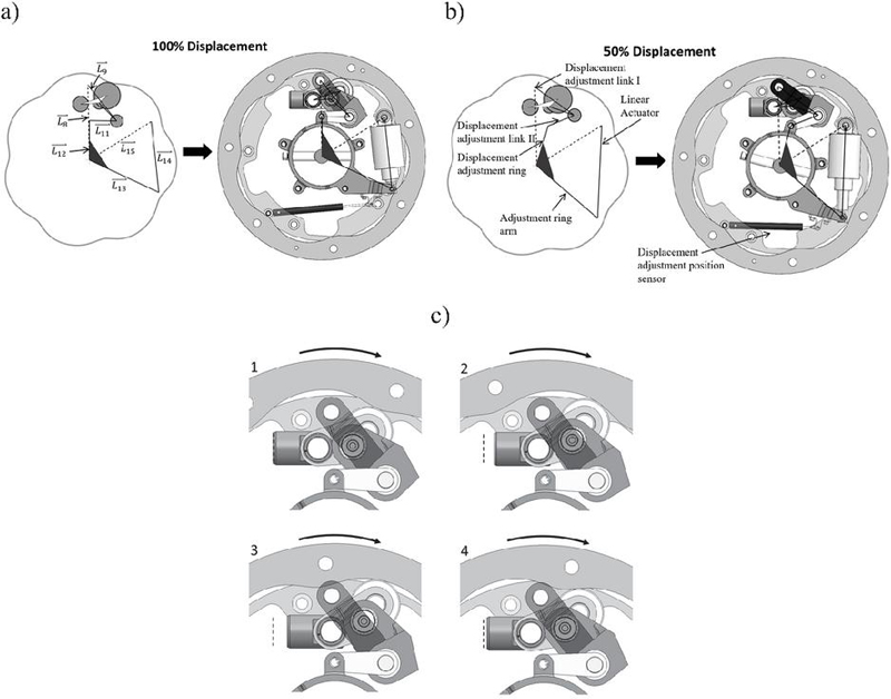
Figure 4 Schematic representation of main linkage mechanism and DAM mechanism. (a) 100% displacement, (b) 50% displacement, (c) animation of main linkage mechanism motion. The dashed line shows the top-dead-centre location of the piston.

2.6 Variable Displacement Linkage Motor Prototype

The models previously developed are applied to analyse the displacement adjustment mechanism of a prototype low-speed high-torque variable displacement linkage motor. The prototype has five pistons mounted on a single radial plane, a seven-lobed main cam mounted in a rotating case, a bore-to-stroke ratio of 2.5, and variable displacement capability from 150 cc/rev – 300 cc/rev. Figures 4(a) and 4(b) show the schematic representation of the linkage mechanisms along with the CAD model at two different displacements. For simplicity, only one main linkage mechanism is shown. The name and nomenclature of some components are also included in these figures. The rocker, the displacement adjustment links, and the linear actuator are represented by solid lines, the coupler link is shown as a triangular shape, the joint bearings of the main linkage mechanism are represented by circles, and the cam roller follower is the largest diameter circle. The circle diameters represent the external size of the bearings/roller followers used in that specific joint. The piston geometry is not included but the piston wrist pin bearings are represented by circles. The joints of the displacement adjustment mechanism are not in constant motion, for this reason, plain bearings are used in the pin joints instead of roller bearings. When the displacement is decreased, the linear actuator ${\mathit{l}}_{\mathbf{14}}$ is extended and the displacement adjustment ring rotates in the clockwise direction moving the position of the adjustable ground pivot. The opposite motion happens when the displacement is increased. A hall effect position sensor located between the DAM ring and the ground is used to measure the motor displacement. Figure 4(c) shows a motion animation of the main linkage mechanism for 100% displacement. In this figure, four positions are shown illustrating the contact points between the rotating cam and the roller follower, and the distance between the piston and TDC.

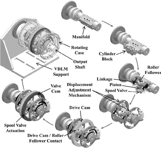
Figure 5 CAD design of variable displacement linkage motor.

Figure 5 shows the virtual assembly of the VDLM motor, which for visualization purposes, only includes one of the five main linkage-cylinder block assemblies. The first component in the assembly is the manifold which remains in static position and is bolted to the motor support. The manifold includes fluid lines for the operation of the motor and the fluid lines to actuate the displacement adjustment mechanism. Next, the figure shows a cylinder block, and a main linkage mechanism mounted on the manifold. The cam-actuated spool valve responsible for regulating the valve timing and valve area is mounted on the cylinder block. Subsequently, the displacement adjustment mechanism is attached on both sides of the cylinder block. The drive cam is in contact with the roller follower of the main linkage mechanism. The valve cam is mounted next to the drive cam. The spool valve undergoes radial motion as it contacts the valve cam. Both cams and the output shaft are mounted on the rotating case. The rings rotate around the circular manifold which is in a static position. Table 1 shows the linkage mechanism parameters used in the model.

Table 1 VDLM motor: linkage mechanism parameters

Design Parameter	Value	Design Parameter	Value
Number of pistons, $n$	5	Number of cam lobes, m	7
Piston diameter, $\mathrm{\varnothing }$ $[m]$	0.030	$m_2$ $[kg]$	0.2
Stroke $s_{max}[m]$	0.012	$m_3$ $[kg]$	1.60
$l_3$ $[m]$	0.0312	$I_3$ $[kg.m^2]$	7.6$\times$10-4
$l_4$ $[m]$	0.0429	$m_4$ $[kg]$	1.79
$l_5$ $[m]$	0.0473	$I_4[kg.m^2]$	1.0$\times$10-3
$l_6$ $[m]$	0.0186	$m_9$ $[kg]$	0.682
$l_7$ $[m]$	0.0784	$I_9[kg.m^2]$	5.4$\times$10-4
$l_8$ $[m]$	0.0809	$m_{11}$ $[kg]$	0.164
$l_9$ $[m]$	0.0784	$I_{11}$ $[kg.m^2]$	4.94$\times$10-5
$l_{10}$ $[m]$	0*	$m_{13}$ $[kg]$	4.06
$l_{11}$ $[m]$	0.0464	$I_{13}[kg.m^2]$	1.25$\times$10-3
$l_{12}$ $[m]$	0.0670	$m_{14}$ $[kg]$	2.29
$l_{13}$ $[m]$	0.1302	$I_{14}[kg.m^2]$	2.30$\times$10-3
$l_{14}$ $[m]$ (100% disp.)	0.1210	$l_{14}$ $[m]$ (50% disp.)	0.15
$l_{15}$ $[m]$	0.1240
*For this specific mechanism configuration ${\mathit{l}}_{\mathbf{10}}=\mathbf{0}$.

2.7 Experimental Setup

To conduct experimental testing on the VDLM motor, a test stand with two hydrostatic transmissions (HST) was built. The first HST generates an adjustable load which is applied to the VDLM shaft. The Second HST comprises the VDLM motor and a pump that delivers flow to the VDLM. Both hydrostatic transmissions are powered by an electric motor acting as the prime mover. Additional information related to the design of the test stand can be found in reference [3]. An additional hydraulic circuit was designed to control the DAM mechanism. As shown in Figure 6, this circuit includes a supply pressure of 10.34 MPa (1500 psi), a servo valve, two hydraulic cylinders, two pressure sensors (Omega PX4201-3KGV, range: 0–3000 psi, sensitivity: 10 mV/V, accuracy: $\pm$0.25% of full scale) used to indirectly measure the actuation force, and a calibrated Hall effect position sensor (Active Sensors MHL1122, stroke: 100 mm, resolution: 0.025 mm, calibrated accuracy: $\pm$1 mm) for tracking the position of the hydraulic cylinders. A proportional-integral (PI) controller implemented with Simulink^® Desktop Real-Time^TM is used to control the position of the DAM mechanism. Figure 7 shows the test stand used for experimental validation.

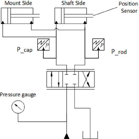
Figure 6 Simplified hydraulic circuit schematic of displacement adjustment circuit.

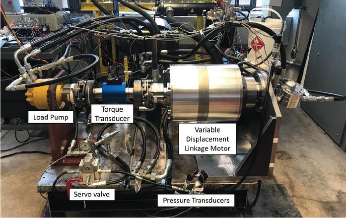
Figure 7 Experimental testing of VDLM prototype.

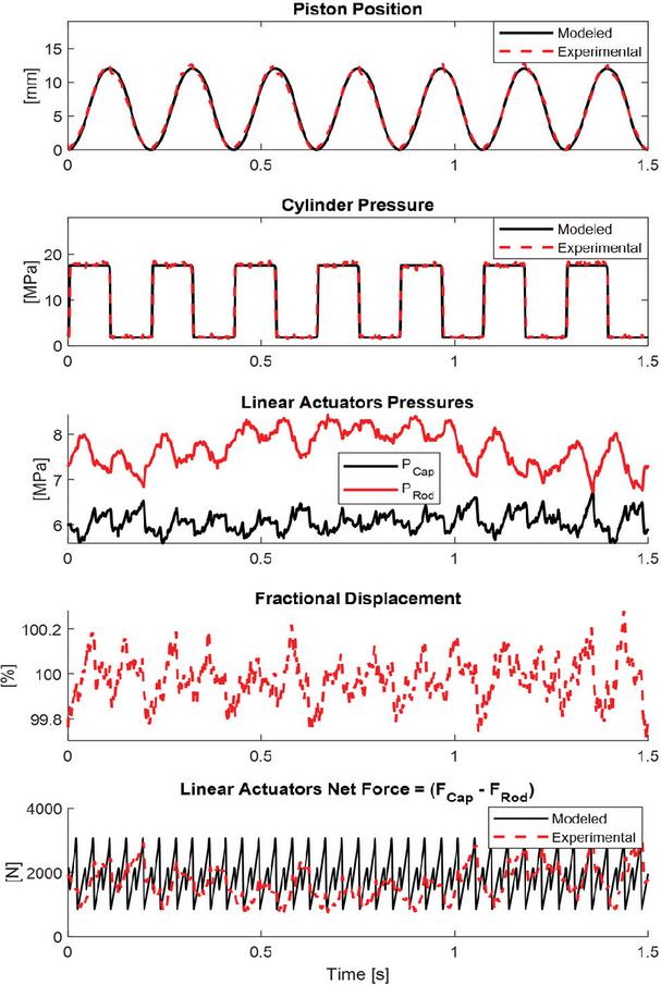
Figure 8 Experimental Data at 40 rpm, motoring forward, displacement 100%.

3 Results

3.1 Constant Displacement Results

Figure 8 shows the experimental and model-predicted results for 100% displacement. The first row shows a comparison between modelling and experimental results of piston position for one complete motor revolution. The second row shows a comparison between modelling and experimental results of cylinder pressure. The piston position and the cylinder pressure are measured on a single instrumented cylinder. The third row shows the fluid pressures at the cap side and the rod sides of the linear actuators. These pressure measurements are used to indirectly calculate the net actuator force for different displacements. The fourth row shows the measured displacements, which appear to be relatively constant with small oscillations. The last row shows a comparison between modelling and experimental results of the actuator’s forces for one complete motor revolution. At 100% displacement, the experimental actuator force is 1664.9 N, the force calculated with the model is 1859.6 N and the difference of the experimental value with respect to the model is 10.5%. Because the displacement is constantly adjusted to keep the desired value, it was assumed that the actuators are in constant motion, and a kinetic friction coefficient was applied to all the joints. When the mechanism oscillates in both directions, the frictional forces switch signs, and a small band is created with a maximum and a minimum force to set the desired displacement. The linear actuator force was calculated as the average of these two forces. Furthermore, the linear actuator force is not constant and has 5 peaks per piston cycle (35 peaks per motor revolution).

3.2 Variable Displacement Results

Figure 9 shows the simulation results of dynamic displacement adjustment for a single piston. The linear actuator extends, and the piston stroke changes from 100% to 50%, in 0.3 s. The figure also shows the change in the piston’s top dead centre position (lower peaks) and bottom dead centre position (upper peaks) for different displacements. The same figure shows the calculated cylinder pressure dynamics, the linear actuator force, and the output torque corresponding to a single cylinder. The linear actuator force is calculated with and without inertial and frictional forces. The actuator force is signed, and a positive force corresponds to an extension force. The calculated torque considers the energy losses by friction on different joints and is slightly smaller than the ideal motor torque calculated with the Equation (38). The output torque is negative because the motor is rotating in a clockwise direction. A comparison between the ideal torque, calculated from a power balance, and the torque calculated from the simulation is useful to confirm that the dynamic model is working properly.

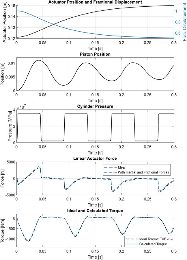
Figure 9 Dynamic displacement adjustment from 100 to 50%: several operating parameters for a single piston (96 rpm, $\mathrm{\Delta }$p $=$ 33 MPa, and adjustment time $=$ 0.3 s).

Figure 10 illustrates the impact of inertial forces on the actuation force for three different adjustment times, comparing scenarios where the displacement is decreased (Figure 10(a)) versus increased Figure 10(b). When the displacement is decreased, as shown in Figure 10(a), the maximum actuation force with a settling time of 19 ms is 55.8% larger than the maximum force at a constant 100% displacement. Similarly, Figure 10(b) shows the effect when the displacement increases from 50% to 100%. The peak actuation force at a 19 ms settling time is 12.6% higher than the maximum force at a constant 50% displacement.

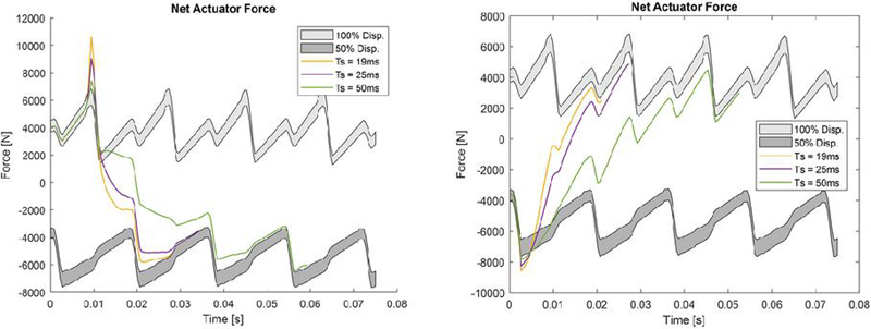
Figure 10 Effect of adjustment time in actuation forces, 96 rpm and $\mathrm{\Delta }$p $=$ 33 MPa. (a) adjustment from 100 to 50%, (b) adjustment from 50 to 100%.

Figure 11 shows the maximum magnitude of the actuation forces for two operating pressures and several motor speeds and settling times. As expected, smaller settling times increase the actuation forces. Furthermore, when the displacement is decreased, the dynamic forces are much larger than the forces generated when the displacement is increased.

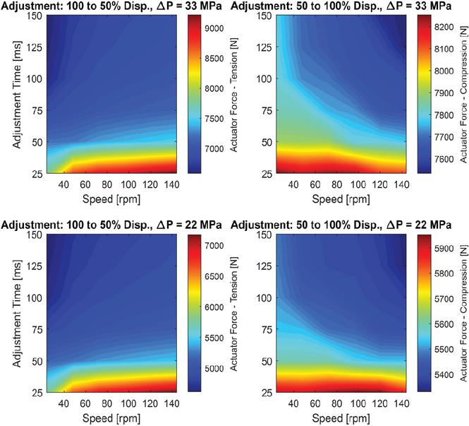
Figure 11 Actuation forces for different motor speeds and adjustment times (motoring forward – clockwise).

If the two actuators are chosen for a settling time ${\mathit{T}}_s=25$ ms, and an actuator operating pressure of 13.79 MPa (2000 psi), the minimum areas required for extension and retraction would be ${\mathit{A}}_{\mathit{c}\mathit{a}\mathit{p}}=328$ mm², ${\mathit{A}}_{\mathit{r}\mathit{o}\mathit{d}}=299$ mm². Assuming a common ${\mathit{A}}_{\mathit{c}\mathit{a}\mathit{p}}/{\mathit{A}}_{\mathit{r}\mathit{o}\mathit{d}}$ ratio of 1.5 and using ${\mathit{A}}_{\mathit{r}\mathit{o}\mathit{d}}$ for the calculation, the minimum cap side area would be 448 mm². This would require a servo hydraulic circuit with a flow rate of 137 l/min as shown in Figure 12 to reduce the displacement from 100 to 50%. The same figure also shows the flow rate requirement for a settling time ${\mathit{T}}_{\mathit{s}}=50$ ms.

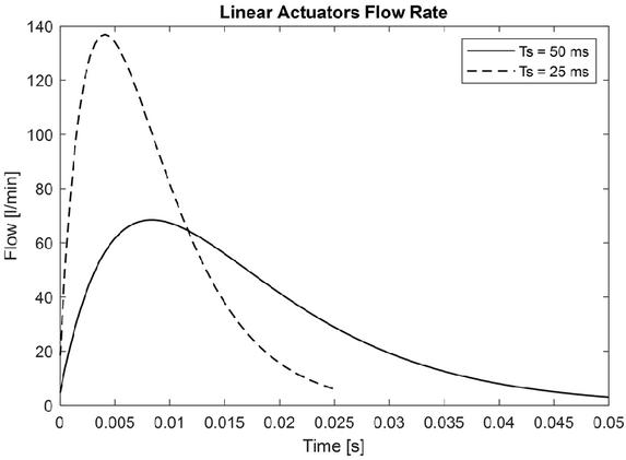
Figure 12 Actuator flow rate for different settling times.

4 Discussion

Figure 8 shows good agreement of piston position for an entire motor revolution. The minor differences in piston trajectories observed were due to linkage deflection, which increased the piston stroke. A cam inspection was not performed but the differences in piston stroke are cyclical and correspond exactly with the number of cam lobes. Figure 8 also shows good agreement of the cylinder pressure dynamics for an entire motor revolution. There appear to be minor differences in the pressure rise and fall, probably due to minor differences in the cam lobe geometries or stack-up errors in the mechanism assembly. Both the piston position and the cylinder pressure were only measured in a single cylinder; therefore, it is not possible to know what happened with the other piston-cylinder assemblies. Figure 8 also includes the pressure measurements on the cap side and the rod side of the linear actuators. These measurements were used to calculate the net force on the linear actuators for motor operation at constant speeds. The measured displacement, shown in the same figure, indicates that the closed loop controller worked properly setting the displacement within $\pm$0.2% of the specified value. Moreover, there is a maximum difference of 10.47% of the measured actuator force with respect to the model. This difference could be due to poor accuracy of the indirect force measurement, or minor differences in the valve timing, which alters the cylinder pressure dynamics, and the forces exerted on the motor. Nevertheless, the experimental values show that the magnitude of the actuation force is close to what was anticipated. Regarding the signature of the actuator force signal, it appears to be directly influenced by the closed-loop position control of the adjustable mechanism. The signature of the fractional displacement signal has similarities with the signature of the actuator force signal. Another important observation is that the undulation of the force signal seen in Figure 8 is repeated every revolution. This undulation has been previously found in torque measurements of hydraulic motors [26] and in the case of this prototype, it may be attributed to minor disparities in the fabrication of each cam lobe or linkage assembly.

Figure 10 shows the increase in dynamic forces as the adjustment time is decreased. For the same operating conditions, the dynamic forces are greater when displacement is decreased compared to when it is increased. This is most noticeable at the beginning of the adjustment, where the mechanism starts at high displacement and undergoes rapid motion. The larger accelerations and longer travel distances at this stage result in higher inertial forces during displacement reduction. Furthermore, the net actuator force is not constant and has five maximum peaks per piston cycle, which correspond with the number of pistons of the motor. All the signals at different settling times match the forces at constant displacements at the beginning and the end of the cycle. This is useful to confirm that the dynamic models are working properly.

The magnitude of dynamic forces for dynamic displacement adjustment becomes important for adjustment times smaller than 75 ms, especially for displacement reduction. Faster motor speeds slightly increase the actuation forces for 100% displacement and slightly decrease the actuation forces for 50% displacement. The inertial forces become increasingly important compared to the pressure forces when the motor pressure decreases. For instance, at $\mathrm{\Delta }$p $=$ 33 MPa and 148 rpm, there is a force increase of 33.33% when the settling time is decreased from 150 to 25 ms. Whereas at $\mathrm{\Delta }$p $=$ 22 MPa and 148 rpm, there is a force increase of 47.1% when the settling time is decreased from 150 to 25 ms.

5 Conclusion

This paper contributes to the literature by presenting the dynamic modelling, experimental validation, and analysis of the adjustable mechanism for a variable displacement linkage motor. The mathematical models considered the kinematic and dynamic equations of the displacement adjustment mechanism and the cylinder pressure dynamics of the hydraulic motor. The analysis was divided into two parts. The first part analysed the hydraulic motor at constant displacement settings and validated the models with experimentation. The second part studied dynamic displacement adjustment changes and determined the effect of different adjustment times and motor speeds on the actuation forces.

The results of the dynamic analysis show that the inertial forces are higher when the displacement is decreased versus increased. This is because the mechanism is subjected to higher accelerations when the displacement is at its maximum. Furthermore, when the adjustment time is below 75 ms, the inertial forces start to become relevant. When the adjustment time is decreased from 50 ms to 19 ms, the maximum actuation forces increase by 75.6% at 96 rpm and $\mathrm{\Delta }$p $=$ 33 MPa.

It was demonstrated that the adjustment speed is limited by the flow rate of the servo-hydraulic system. Greater actuation speeds result in increased forces, necessitating actuators with larger diameters and thus demanding higher flow rates. Further work can be directed towards optimizing the mechanism to decrease both the actuator size and the necessary flow rate for the servo-hydraulic circuit.

All the metrics evaluated in this paper such as dynamic forces vs. adjustment times, and servo-hydraulic circuit parameters can contribute to a deeper understanding of how an adjustable low-speed high torque motor can be used in potential applications such as series hybrid hydrostatic transmissions.

Acknowledgement

This material is based upon work supported by the U.S. Department of Energy’s Office of Energy Efficiency and Renewable Energy (EERE) under the Vehicle Technologies Office Award Number DE-EE0008335. Disclaimer: “This report was prepared as an account of work sponsored by an agency of the United States Government. Neither the United States Government nor any agency thereof, nor any of their employees, makes any warranty, express or implied, or assumes any legal liability or responsibility for the accuracy, completeness, or usefulness of any information, apparatus, product, or process disclosed or represents that its use would not infringe privately owned rights. Reference herein to any specific commercial product, process, or service by trade name, trademark, manufacturer, or otherwise does not necessarily constitute or imply its endorsement, recommendation, or favouring by the United States Government or any agency thereof. The views and opinions of authors expressed herein do not necessarily state or reflect those of the United States Government or any agency thereof.”

Disclosure

The authors declare that they have no financial interest or benefit arising from the direct applications of this research.

References

[1] M. Ivantysynova, “Displacement Controlled Linear and Rotary Drives for Mobile Machines with Automatic Motion Control,” in International Off-Highway & Powerplant Congress & Exposition, Milwaukee, 2000.

[2] O. Biedermann, J. Engelhardt and J. Geerling, “More Efficient Fluid Power Systems Using Variable Displacement Hydraulic Motors,” Technical University Hamburg-Harburg, Section Aircraft Systems Engineering, Hamburg, 1998.

[3] J. Hartoyo, J. Voth, J. Pozo-Palacios, G. Boyce-Erickson, M. Herrera-Perez, P. Li and J. Van de Ven, “Using a Novel Variable Displacement Linkage Motor to Save Fuel in a Compact Track Loader Drivetrain,” in Fluid Power Systems Technology, Sarasota, 2023.

[4] S. Wilhelm and J. D. Van de Ven, “Design and Testing of an Adjustable Linkage for a Variable Displacement Pump,” Journal of Mechanism and Robotics, vol. 5, no. 4, 2013.

[5] S. Wilhelm and J. D. Van de Ven, “Efficiency Testing of an Adjustable Linkage Triplex Pump,” in ASME Symposium on Fluid Power and Motion Control, Bath, 2014.

[6] N. Fulbright, G. Boyce-Erickson, T. Chase, P. Li and J. Van de Ven, “Automated Design and Analysis of a Variable Displacement Linkage Motor,” in Proceedings of the ASME/Bath Symposium on Fluid Power and Motion Control, Sarasota, 2019.

[7] J. Larson, J. Pozo-Palacios, G. Boyce-Erickson, N. Fulbright, J. Dai, J. Voth, N. Gajghate, J. Saikia, P. Michael, T. Chase and J. Van de Ven, “Experimental Validation of Subsystem Models for a Novel Variable Displacement Hydraulic Motor,” in ASME/BATH 2021 Symposium on Fluid Power and Motion Control, Virtual, 2021.

[8] J. Pozo-Palacios, J. Voth and J. Van de Ven, “Kinematics of an Adjustable Cam-Linkage Mechanism for a Variable Displacement Hydraulic Motor,” in International Design Engineering Technical Conferences and Computers and Information in Engineering Conference, Boston, 2023.

[9] J. Pozo-Palacios, N. Fulbright, J. Voth and J. Van de Ven, “Comparison of Forward and Inverse Cam Generation Methods for the Design of Cam-Linkage Mechanisms,” Mechanism and Machine Theory, vol. 190, no. 105465, 2023.

[10] M. Herrera-Perez, G. Boyce-Erickson, J. Pozo-Palacios, J. Voth, P. Michael and J. Van de Ven, “Torque Ripple Minimization in a Variable Displacement Linkage Motor (VDLM) Through the Customization of Piston Trajectory,” in Proceedings of the BATH/ASME 2024 Symposium on Fluid Power and Motion Control, Bath, 2024.

[11] G. Zeiger and A. Akers, “Torque on the Swashplate of an Axial Piston Pump,” Journal of Dynamic Systems, Measurement and Control, vol. 107, no. 3, pp. 220–226, 1985.

[12] G. J. Schoenau, R. T. Burton and G. P. Kavanagh, “Dynamic Analysis of a Variable Displacement Pump,” Journal of Dynamic Systems, Measurement and Control, vol. 112, no. 1, pp. 122–132, 1990.

[13] N. Manring and V. Mehta, “Physical Limitations for the Bandwidth Frequency of a Pressure Controlled, Axial’Piston Pump,” Journal of Dynamic Systems, Measurement and Control, vol. 133, no. 6, 2011.

[14] P. Nikravesh, Computer-Aided Analysis of Mechanical Systems, New Jersey: Prentice Hall, 1988.

[15] R. Norton, Design of Machinery, Worcester: McGraw-Hill, 1999.

[16] S. Wilhelm, “Modeling, Analysis and Experimental Investigation of a Variable Displacement Linkage Pump,” University of Minnesota, Minneapolis, 2015.

[17] A. Erdman and G. Sandor, Advanced Mechanism Design, Analysis and Synthesis, Upper Saddle River, NJ: Prentice Hall, 1997.

[18] R. Norton, “Acceleration Analysis: Acceleration of Any Point on a Linkage,” in Design of Machinery, Boston, McGraw-Hill, 1999.

[19] B.-H. Cho, H.-L. Lee and J.-S. Oh, “Estimation Technique of Air Content in Automatic Transmission Fluid by Measuring Effective Bulk Modulus,” in FISITA World Automotive Congress, Seoul, 2000.

[20] N. Manring, “Fluid Mechanics,” in Hydraulic Control Systems, Hoboken NJ, John Wiley & Sons, 2020, p. 50.

[21] JTEKT Corporation, “Bearing Knowledge: Rolling Bearing Friction, Tech. Cat. No. CAT.B2001-8,” Koyo Bearings (JTEKT Corporation), Osaka, 2001.

[22] R. T. Barrett, “Fastener Design Manual, NASA RP-1228,” NASA Lewis Research Center, Cleveland, 1990.

[23] J. Xia and W. Durfee, “Modeling of Tiny Hydraulic Cylinders,” in 52nd National Conference in Fluid Power, Las Vegas, 2011.

[24] F. Al-Ghathian and M. Tarawneh, “Friction Forces in O-Ring Sealing,” American Journal of Applied Sciences, vol. 2, no. 3, pp. 626–632, 2005.

[25] Parker, Parker O-Ring Handbook ORD 5700, Cleveland: Parker O-Ring & Engineering Seals Division, 2021.

[26] Innas BV, “Performance of Hydrostatic Machines,” Innas BV, Breda, 2020.

Biographies

Jonatan Pozo-Palacios is a postdoctoral associate at the University of Minnesota, where he conducts research at the Mechanical Energy and Power Systems (MEPS) Laboratory. He earned his PhD in Mechanical Engineering from the University of Minnesota in 2024. His research focuses on model-driven design of fluid power systems.

Grey C. Boyce-Erickson earned his BSME from the University of Minnesota and is currently pursuing a PhD in Mechanical Engineering at UMN. His research at the Mechanical Energy and Power Systems (MEPS) Laboratory focuses on hydraulic valves and valve timing.

Justinus K. Hartoyo is an international student from Indonesia. He obtained his bachelor’s degree in biomedical engineering from the University of Minnesota in 2016. Justinus then started his doctorate program in Mechanical Engineering in 2018 at the same institution, where he currently resides. His research focuses on construction vehicle system-level control and optimization.

Martin Herrera-Perez completed his B.S in mechanical engineering at the University of Miami in 2020. Currently, he is a Ph.D. student who works as a research assistant at the Mechanical Energy and Power Systems laboratory at the University of Minnesota. Martin’s research interests are in model-driven design of fluid power systems and efficient energy conversion with emphasis on flow and torque ripple minimization.

John A. F. Voth received his BSME from Oral Roberts University in 2018 and is currently pursuing his PhD in mechanical engineering from the University of Minnesota (UMN). He researches at the Mechanical Energy and Power Systems (MEPS) Laboratory at UMN, and his research interests include mechanism design, optimization of machines, energy conservation, and hydraulics.

James D. Van de Ven is a Professor at the University of Minnesota in the Department of Mechanical Engineering where he operates the Mechanical Energy and Power Systems (MEPS) Laboratory. Dr. Van de Ven’s research interests are in efficient energy conversion, energy storage, fluid power, kinematics, and machine design.

International Journal of Fluid Power, Vol. 26_4, 539–572
doi: 10.13052/ijfp1439-9776.2642
© 2025 River Publishers