Defining the Design Space of Basic Hydraulic Drive Networks

Mikkel van Binsbergen-Galán^* and Lasse Schmidt

AAU Energy, Aalborg University, Aalborg, Denmark
E-mail: mbg@energy.aau.dk
*Corresponding Author

Received 19 May 2025; Accepted 17 July 2025

Abstract

Hydraulic systems are widely used throughout industry to actuate and control applications where large forces are required. These applications include off-highway machinery like excavators, loaders, manufacturing machinery like presses, injection molding machinery and so forth. With a continuously increasing focus on electrification and reduced energy consumption, emissions and rare earth material usage, energy efficiency, reduced component sizes and limited component numbers become increasingly important. In this endeavor, the recently introduced concept of hydraulic drive networks appears especially feasible to consider in applications with two or more hydraulic actuators to be controlled. Key features of hydraulic drives networks are the sole use of displacement units as flow control elements, absence of traditional control valves, and short-circuiting of hydraulic actuator chambers, while maintaining the possibility of individual control of each actuator. A consequence of these features is that possible ways of connecting the flow ports of displacement units to those of the actuators increases exponentially with the number of actuators to be controlled, rendering the use of traditional hydraulic system design methods obsolete. A possible way to systematically characterize and identify feasible networks is by use of graph theory. However, at this stage, no standardized approaches and definitions exist for such systems. This paper considers the concept of hydraulic drive networks in the framework of graph theory and applies the concept of tree-graphs to define the design space of feasible hydraulic drive network architectures for any number actuators constituting a number of control volumes for which flow must be controllable. Identifying and distinguishing each architecture in the design space is vital in the process of hydraulic drive network design, for being able to compare and optimize architectures based on objectives such as size, cost, efficiency and so forth.

Keywords: Hydraulic drive network, design space, system design, structural controllability, modeling.

1 Introduction

Hydraulic systems are used as a means of power transfer enabling control of power flows in applications which require e.g., high forces, robustness against impact loads, precise dynamic control, and high power density. Applications include injection molding machines, presses, excavators, loaders, cranes and alike, where hydraulic actuators enable motion or force control. Current trends involve energy efficiency improvements allowing to reduce energy consumption and associated emissions which, in turn, enables electrification, battery powered operation etc. [1, 2, 3]. Common for many hydraulic systems is poor energy efficiency which entails significant pollution, especially in off-highway machines as these are commonly powered by internal combustion engines [4].

An approach to increase energy efficiencies is by controlling the fluid flow in hydraulic actuators directly by displacement units thereby limiting or avoiding the use of traditional control valves, thereby limiting throttle losses [3, 5, 6, 7, 8]. Even though many systems contain several actuators in terms of hydraulic cylinders and/or hydraulic motors, focus in this area has primarily been related to standalone hydraulic actuator solutions. Nevertheless, performance of a system can be improved if a network architecture can be designed specifically with the aim of making the system amenable to control [9]. This is, however, seldom the case for industrial hydraulic systems. On the contrary, hydraulic systems may be designed for the mechanism they are to actuate and hence, they can and should be designed to enable control and, additionally, optimized for e.g., size, number of components, and performance. The concept of networks has been widespread in other engineering fields, but has not yet received the same attention within the field of hydraulic systems. Only recently this was considered by [3], introducing the idea of making connections between several hydraulic displacement units and actuators realizing so-called hydraulic drive networks.

Hydraulic drive networks are essentially coordinated drive systems enabling the control of multi-actuator systems, alternative to controlling each actuator individually. Both dual actuator hydraulic drive network architectures [3, 10, 11, 12] and triple actuator hydraulic drive network architectures [13] have been studied until now. It is, however, not clear how to derive the most feasible architecture in view of certain design constraints. Some of the hydraulic drive networks presented in literature are shown to include fluid short circuit connection between actuator chambers which effectively reduces the number of separate control volumes to which flow must be individually controllable. The ability to comprehensively identify and distinguish different system architectures is vital in the design process of a system, to be able to systematically compare different system architectures and find the optimal architecture based on design objectives such e.g. component sizes and energy efficiency.

This paper presents a comprehensive approach for defining and identifying the design space for any number of control volumes. The design space consists of every hydraulic drive network with the minimum number of needed drives, which is physically sensible to apply to a system. This approach applies methods from graph theory while considering the physical adaptions needed when considering hydraulic drive networks.

2 Conceptualization of a Hydraulic Drive Network

A hydraulic drive network (HDN) is composed of a number of control volumes (fluid volumes in which flow/pressure must be independently controllable), at least one fluid reservoir, and a number of hydraulic displacement machines interconnecting the volumes. An example of a dual actuator (cylinder) HDN is shown on Figure 1. The hydraulic displacement machines in an HDN are connected directly to the adjacent volumes without any other components in the path i.e., the hydraulic system may be categorized as direct operated. Valves could be used for realizing safety and other supplementary functionalities, but the main functionality should be independent of valves and other hydraulic components.

2.1 Key Element in Hydraulic Drive Networks

The key elements of a hydraulic drive network, regardless of the number of actuators, are control volumes, fluid reservoirs and hydraulic displacement machines. For clarity in the subsequent sections, the interpretation of these key elements are described in the following.

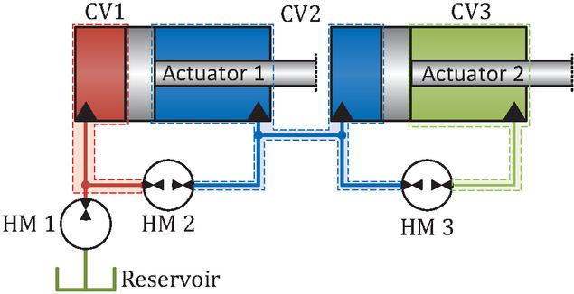
Figure 1 Example of a dual actuator hydraulic system with indications of control volumes (CV), hydraulic displacement machines (HM), and reservoir.

2.1.1 Control Volume (CV)

In an HDN, a control volume is defined as any enclosed hydraulic volume to which it is possible to direct flow in an independent manner without affecting any other control volume. A control volume may be any type of fluid volume, though it is most meaningful to relate a control volume to hydraulic actuators, e.g., each chamber of a hydraulic cylinder or hydraulic motor. Furthermore, a control volume may also be a collection of several individual chambers if these have been short circuited in a way that allows for all machine functionalities. This is the case in the HDN example in Figure 1 where the rod-side chamber of actuator 1 and the piston-side chamber of actuator 2 (the blue colored chambers) combine as control volume 2 (CV2). A control volume contains both the actuator volume as well as hoses and pipe connections which may constitute a significant part of the total control volume.

2.1.2 Reservoir Volume

A fluid reservoir is needed in HDNs to account for changes in total system volume (the sum of all control volumes), fluid compression, and fluid leakage. In addition, a fluid reservoir may be used for thermal management and filtration of the fluid similar to traditional hydraulic systems. A reservoir volume may be realized as e.g. a hydraulic fluid tank or an accumulator. Such a reservoir is not considered a control volume since the possible pressure variation is limited and generally not a control objective. Figure 1 shows an example of a hydraulic drive network for 3 control volumes and 1 reservoir in the form of a fluid tank.

2.1.3 Hydraulic Displacement Machine (HM)

The interconnections between control volumes are comprised of any type of hydraulic displacement machine for which flow can be controlled in four-quadrant operation, meaning bidirectional flow regardless of the flow port pressures, allowing the power transmitted to be both positive and negative. In addition, the interconnection between a control volume and a reservoir volume is comprised by any type of hydraulic displacement machine allowing for two-quadrant operation, i.e. bidirectional flow with high pressure only in one of the flow ports. A hydraulic displacement machine could be any type of hydraulic flow displacing unit that can act as both a flow source and a flow sink, in the sense that it can create a flow between two volumes to which it is connected. When combined with its power source i.e. a prime mover (e.g., en electric machine and associated electric drive) the hydraulic displacement machine is considered a hydraulic drive.

2.2 Basic Hydraulic Drive Networks

A hydraulic drive network, or HDN, could in general contain any number of drives, up to the point where every control volume is connected to all other control volumes (a so-called fully connected network [3]) However, increasing the number of drives also increases the complexity and cost of the network. Therefore, the following two properties may be favorable when focusing on the main functionality of a machine:

1. The system output states are individually controllable.

2. The system has a minimum number of drives given a number of control volumes to allow 1).

If these two properties are fulfilled in an HDN, when considering the main machine functionality, it is defined to be a basic HDN.

The motivation for the first property is self-evident since an uncontrollable system is not feasible as a working machine. The second property is motivated by system cost and simplicity, considering that the main functionality can be accomplished with a limited number of drives. If there are additional drives, these are non-essential to the main machine functionality and thus an unnecessary cost. Other considerations, besides the main functionality of the machine, may justify an increase in the number of drives such as: fluid conditioning; system reliability; and accounting for auxiliary machine functionalities. Such considerations are beyond the scope of this paper and are hence not considered further here.

3 Modeling and Controllability of Basic Hydraulic Drive Networks

The generic flow continuity equation used to describe the pressure dynamics for a control volume, is given as Equation 1 (neglecting flow losses), with $\mathit{C}$ being the hydraulic capacitance, $nv$ being the number of control volumes, ${\mathit{q}}_{\mathit{d}}$ being the flows going into the volume, where $q_{d,j}$ is the flow from drive $j$ and $nd$ is the number of drives in the system. The volume change with time, $\dot{V}$, may be regarded as the internal system dynamics. The system dynamics may in general depend on component dynamics (e.g. for a hydraulic accumulator) and mechanical couplings (e.g. in the form of a cylinder as in the example on Figure 2).

$$\begin{array}{cc}& {\dot{p}}_i=\frac{1}{c_i}\left(\sum _j(q_{d,j})-{\dot{V}}_i\right),c_i=\frac{V_i}{{\beta }_i}\hfill \\ & i\in \{1,\mathrm{\dots },nv\},j\in \{1,\mathrm{\dots },nd\},nv,nd\in \mathbb{Z}\hfill \end{array}$$

(1)

The pressure dynamics of a number of control volumes may be considered in a state space form as Equation 2, with $\mathit{T}$ representing a transformation matrix, with entries having one of the values $\{-1,0,1\}$. This is the input matrix (scaled by $\mathit{c}$) which relates how the drives are connected and hence, how they affect the states. The transformation matrix $\mathit{T}$ thus describes the architecture of the drive network. The operator $[\odot ]$ is used to represent element-wise multiplication (also called Schur- or Hadamard-product). The inputs $\mathit{u}$ are the flows from the drives. In the following, matrices are indicated with bold capital symbols, while vectors are indicated with bold lowercase symbols.

$$\begin{array}{cc}\hfill \dot{\mathit{x}}& =\mathit{A}\mathit{x}+\mathit{B}\mathit{u}\hfill \\ \hfill \mathit{x}& =\mathit{p},\mathit{A}=\mathit{A}(\dot{\mathit{V}}),\mathit{B}=\mathit{c}\odot \mathit{T}\hfill \\ \hfill \mathit{c}& ={[\frac{1}{c_1},\mathrm{\dots },\frac{1}{c_i}]}^{\top },\mathit{u}={\mathit{q}}_d\hfill \end{array}$$

(2)

For a state space model, the controllability of the system [14, 15], may be evaluated using the Kalman rank criterion: The controllability matrix $\mathbf{𝒞}$ is given as Equation 3 with controllability being achieved if it has full rank, $\text{rank}(\mathbf{𝒞})=n$, with $n$ being the number of states. Whereas controllability traditionally refers to whether the states of a system are affected by an input due to their structural relations through the system and input matrices, a more explicit form of controllability may be related to whether the outputs are statically influenced by the input. Such a condition may be expressed by neglecting the system matrix when evaluating controllability. Using this condition, the controllability matrix reduces simply to Equation 4, i.e. the input matrix $\mathit{B}$.

This more conservative controllability matrix can have full rank only if the input matrix has at least as many columns, hence inputs, as there are hydraulic states (number of control volumes). Therefore, at least $nv$ number of inputs are needed ($nd\ge nv$) to enable controllability of the pressure states. When controllability is achieved with the fewest possible number of hydraulic displacement machines, the input matrix $\mathit{B}$ is square, and the system is considered a basic HDN ($nd=nv$).

	$\mathbf{𝒞}=\left[\begin{array}{c}\hfill \mathit{B}\mathit{A}\mathit{B}\mathrm{\dots }{\mathit{A}}^{\mathit{n}\mathbf{1}}\mathit{B}\hfill \end{array}\right]$	(3)
	${\mathbf{𝒞}|}_{\mathit{A}=\mathbf{0}}=\mathit{B}$	(4)

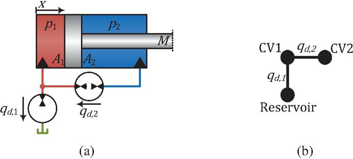
Figure 2 Sketch of example system with two control volumes and two hydraulic displacement machines. (a) Hydraulic schematic. (b) Equivalent graph representation.

3.1 Example: Controllability of an HDN

As an example, the simple system depicted in Figure 2 with one cylinder is analyzed. The corresponding state space model is given by Section 3.1. Note, that the positive flow direction is chosen towards the volume with the lowest label number.

$$\text{rank}(\mathbf{𝒞})=\text{rank}([\mathit{B}\mathit{A}\mathit{B}{\mathit{A}}^{\mathbf{2}}\mathit{B}{\mathit{A}}^{\mathbf{3}}\mathit{B}])=4$$

The rank of the controllability matrix is 4 (Equation 5), implying that the system is controllable when considering the full system dynamics.

$$\text{rank}(\mathbf{𝒞})=\text{rank}([\mathit{B}\mathit{A}\mathit{B}{\mathit{A}}^{\mathbf{2}}\mathit{B}{\mathit{A}}^{\mathbf{3}}\mathit{B}])=4$$

(5)

Neglecting the motion dynamics of the piston, the state space model appears as Equation 6, with the system matrix ${\mathit{A}}^{\prime }$ being a null matrix. This reduced system thus has no internal dynamics and it is analogous to modeling two mechanically non-coupled hydraulic control volumes. The system Equation 6 has two (flow) inputs, one for each control volume which is the minimum necessary to enable control of the pressures. The rank of the controllability matrix of the system Equation 6 is found as Equation 7 implying that controllability is still achieved when considering this reduced system model and neglecting any internal system couplings. This is therefore an example of a basic HDN.

$$\begin{array}{c}\hfill \stackrel{{\dot{\mathit{x}}}^{\prime }}{\left[\begin{array}{c}\hfill {\dot{p}}_1\hfill \\ \hfill {\dot{p}}_2\hfill \end{array}\right]}=\stackrel{{\mathit{A}}^{\prime }}{\left[\begin{array}{cc}\hfill 0\hfill & \hfill 0\hfill \\ \hfill 0\hfill & \hfill 0\hfill \end{array}\right]}\stackrel{{\mathit{x}}^{\prime }}{\left[\begin{array}{c}\hfill p_1\hfill \\ \hfill p_2\hfill \end{array}\right]}+\stackrel{{\mathit{c}}^{\prime }}{\left[\begin{array}{c}\hfill \frac{1}{c_1}\hfill \\ \hfill \frac{1}{c_2}\hfill \end{array}\right]}3-4.0pt\odot 3-4.0pt\stackrel{{\mathit{T}}^{\prime }}{\left[\begin{array}{cc}\hfill 1\hfill & \hfill 1\hfill \\ \hfill 0\hfill & \hfill 1\hfill \end{array}\right]}\stackrel{{\mathit{u}}^{\prime }}{\left[\begin{array}{c}\hfill q_{d,1}\hfill \\ \hfill q_{d,2}\hfill \end{array}\right]}\hfill \\ \hfill {\mathit{B}}^{\prime }={\mathit{c}}^{\prime }\odot {\mathit{T}}^{\prime }\hfill \end{array}$$

(6)

$$\text{rank}({\mathbf{𝒞}}^{\prime })=\text{rank}({\mathit{B}}^{\prime })=2$$

(7)

4 Graph Theory in the Context of Hydraulic Drive Networks

It is desired to obtain a generic method for uniquely identifying all possible basic HDNs for any given system. This is achieved by realizing how hydraulic drive networks may be described by the formal language of graph theory, so that common graph-theoretical concepts become applicable to hydraulic systems. Such methods allow for an encoding scheme to uniquely identify and reference every specific HDN for a given system, which enables easy implementation in a generic and automated computer evaluation program. A brief introduction is given to graph theory to present some of the main concepts which are relevant in this context, taking offset in [16, 17, 18].

4.1 Fundamental Concepts of Graph Theory

A graph (also called a network) is here defined as an ordered pair $\mathcal{𝒢}=\{\mathcal{𝒱},\mathcal{ℰ}\}$ comprising a set of vertices (also called nodes) $\mathcal{𝒱}$ and a set of edges $\mathcal{ℰ}$ (which comprises node pairs), with $\mathcal{𝒱}=\{1,\mathrm{\dots },n\}$ and $\mathcal{ℰ}\subseteq \{\{x,y\}|x,y\in \mathcal{𝒱},x<y\}$. The nodes are entities which are represented graphically by dots, while edges are represented as line connections between two nodes, as seen on Figure 3. In general, an edge may be directed or undirected, meaning whether a connection is unidirectional or bidirectional. A graph with $n$ nodes is said to be of size $n$ ($n$-graph).

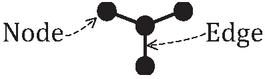
Figure 3 Example of an unlabeled connected graph with 4 nodes and 3 edges with designation of a node and an edge.

A component is a part of a graph where there exists a path from any node to another within that component. If a graph contains only a single component it is said to be connected.

An edge list is the collection of all edges into a two-column matrix where each row defines a start- and end-node for an edge using the node labels. For undirected edges the column entries in each row are interchangeable.

The degree of a node is a measure of how many edges are connected to it, which can be found by counting how many times the node label appears in the edge list.

A path exists between two nodes if it is possible to traverse from the starting node to the end node through edges and nodes without jumping. A path that has the same start and end node and that goes through at least one other node (without reusing edges) is called a cycle.

A complete graph is one that has the maximum number of edges, so that every node is connected by an edge to every other other node.

The nodes of a graph may be labeled (i.e. numbered) to distinguish nodes from one another. The labels are thus used to refer to specific nodes which makes it possible to describe a graph in a programmatic way. The action of labeling a graph is usually made by assigning sequential numbers to each node resulting in a labeled graph. Examples of labeled graphs on four nodes are shown on Figure 4 with each color representing a label (1 is green, 2 is yellow, 3 is blue, 4 is purple).

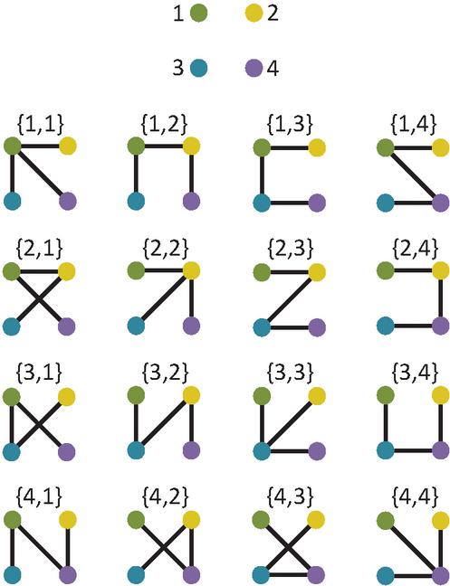
Figure 4 All 4-trees and their Prüfer sequences. In the top of the figure is the relation between numeric labels and color labels (1 is green, 2 is yellow, 3 is blue, 4 is purple). Notice that the position of the nodes stays the same, only the edges change.

All the graphs on Figure 4 are a type of graph called trees. As will become apparent in Section 5, tree-graphs are an important concept in the context of basic networks, and hence considered in more detail in the following.

Table 1 Number of labeled trees on 2-13 nodes as of Cayley’s formula [19].

Nodes	Labeled trees
2	1
3	3
4	16
5	125
6	1,296
7	16,807
8	262,144
9	4,782,969
10	100,000,000
11	2,357,947,691
12	61,917,364,224
13	1,792,160,394,037

4.2 Tree-graphs

A tree is an acyclic connected graph having $n1$ edges. For a tree of size $n$ there are $[n^{(n2)}]$ $n$-trees as of Cayley’s formula [19]. These are all unique (non-isomorphic) labeled trees. The number of unique trees of certain sizes is given in Table 1. All nodes in a tree-graph have degree $\ge 1$. Any tree network may be uniquely identified using a Prüfer sequence $S=\{x_1,\mathrm{\dots },x_{n2}\}$, where $x\in [1,n]$. A Prüfer sequence thus gives complete information about a tree graph in a format implementable in a programming language. From a combinatorial perspective, all Prüfer sequences of an $n$-tree are found by making all $[n2]$-arrangements (with repetitions) of the elements of the set $[1:n]$. For $n=4$, all Prüfer sequences are given on Figure 4 together with the corresponding graph.

The degree of each node in a tree is 1 plus the number of times the label appears in the Prüfer sequence. Nodes in a tree that have degree 1 are called leaves. For the Prüfer sequence $S=\{1,1\}$, node 1 has degree three, since it appears twice in the sequence, while nodes $2$, $3$ and $4$ have degree one. Such a tree, where all nodes but one have degree one, is considered a star tree type, since it has a center node with edges connecting every other nodes.

If the Prüfer sequence has no repeated numbers, e.g., $S=\{2,4\}$, it is a linear tree type where all nodes are connected as a string; the two end nodes have degree one while all nodes inside the string have degree two. The two end nodes are those nodes whose label does not appear in the Prüfer sequence.

If there are some repeated nodes in the Prüfer sequence, but it is not a star tree, it is considered as a branched tree type.

4.3 Coding and Decoding Prüfer Sequences: An Example

For completeness, an example of the coding and decoding of a Prüfer sequence is given. The coding of a Prüfer sequence is a recurrent process of finding the leaf with the lowest node label and noting the label number of the adjacent node and subsequently ignoring that node. Once all nodes but two are ignored the process ends. An example of the coding of a Prüfer sequence is demonstrated in Figure 5.

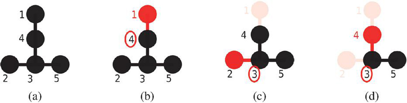
Figure 5 Example of the Prüfer coding process for a 5-tree. The sequential definition of the Prüfer sequence is given according to the figures: (a) $S=\{\}$, (b) $S=\{4\}$, (c) $S=\{4,3\}$, (d) $S=\{4,3,3\}$.

The decoding of a Prüfer sequence is also a recurrent process of drawing edges between pairs of nodes. The edges are drawn by identifying the lowest label number in $L=\{1,2,\mathrm{\dots },n\}$, that is not part of the Prüfer sequence, and joining this node with the first node label in the Prüfer sequence. These two node labels are subsequently ignored. The process stops when there are no more node labels left in the Prüfer sequence, after which the two remaining nodes in $L$ are joined. An example of the decoding of a Prüfer sequence is demonstrated on Figure 6 (note that this is the same graph as in Figure 6(a)) resulting in the edge list Equation 8.

$\mathbf{ℰ}=\left[\begin{array}{cc}\hfill 1\hfill & \hfill 4\hfill \\ \hfill 2\hfill & \hfill 3\hfill \\ \hfill 3\hfill & \hfill 4\hfill \\ \hfill 3\hfill & \hfill 5\hfill \end{array}\right]$

(8)

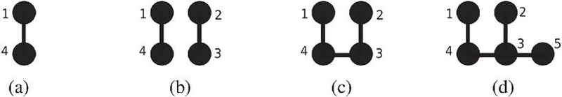
Figure 6 Example of Prüfer decoding of the sequence $S=\{4,3,3\}$ with $L=\{1,2,3,4,5\}$. The sequence of drawing edges is: (a) $e_1=[1,4]$, (b) $e_2=[2,3]$, (c) $e_3=[3,4]$, (d) $e_4=[3,5]$.

5 Hydraulic Networks Interpreted as Graphs

A hydraulic system may be interpreted as a graph by making the simple association that any volume in the network is interpreted as a graph node while any hydraulic displacement machine is interpreted as a graph edge. It is important to distinguish that, while hydraulic displacement machines are often depicted with a circle, when depicting a hydraulic system as a graph its hydraulic displacement machines are depicted with lines to comply with common graph notation. Examples hereof are shown on Figure 2(b). For an HDN graph, the hydraulic displacement machines are assumed to be with bidirectional flow and hence, all edges are considered as undirected.

This interpretation is different from other approaches that deal with controllability of systems and graphs [20, 9, 21, 22, 23] where inputs are seen as nodes in the network (leader nodes) with directional connections to other nodes (follower nodes). Here, however, the system inputs in the form of hydraulic flows are seen as the connections between volumes, hence edges between nodes. This is because a flow source is always seen to have two connection since it needs to draw flow from one volume and supply it to another (much like a current source in an electrical network), thus it is acting between control volumes (graph nodes) in contrast to being an external input. If several sub-volumes are connected to the same outlet they are consequently hydraulically short circuited and thus seen as a single control volume. One could in fact still regard inputs as nodes if one simply puts a (leader) node on every edge, though this only makes the graph more complicated.

Controllability of hydraulic networks, as outlined in Section 3, is a necessary condition when designing such systems. Being interested first and foremost in identifying the possible hydraulic network architectures, this is similar to the notion of structural controllability [24, 25]. Hence, the architecture of a system must allow for controllability in a general way without accounting for the actual values of the system parameters. In a hydraulic network this is achieved when the system graph is connected, which entails that there is a flow path from any control volume to a reservoir volume and that this flow can be controlled through the operation of hydraulic displacement machines.

Additionally, it is considered that only the network architectures with the least amount of drives are of interest. Other works mention similar notions as minimal controllability (in the qualitative sense) [20, 26, 27, 28] though, to reiterate, these works have a different translation between the state space representation of a dynamic system and its equivalent graph. In the interpretation of a graph of a hydraulic drive network, this is analogous to a connected graph with the least amount of edges – which is the definition of a tree-graph. Remember, that one, and only one, of the control volumes must represent a fluid flexing volume in the form of a hydraulic reservoir. Thus, any hydraulic drive network of interest is in the form of a tree and it may be described as minimally structurally controllable; these are basic hydraulic drive networks.

It is possible to identify and index all tree-graphs for a given network size using Prüfer sequences, as outlined in Section 4. The design space of a hydraulic drive network for a given system thus equates to the number of trees for a graph of a given size which is quantified in Table 1 for trees of sizes 2-13 nodes. Though, in practical terms, a system with only one or two control volumes may be too simple to be termed as a network. Considering hydraulic networks to be associated with multi-actuator hydraulic systems, it is expected that there are at least three control volumes plus a fluid reservoir, equivalent to a tree with 4 nodes. This definition allows also for basic HDNs in which several control volumes are connected to the fluid reservoir, which may make it difficult to distinguish a hydraulic drive network from a multi-actuator system which is driven as if it was separate single-actuators. Yet, such networks are not excluded for the generality of the method and with the motivation of being able to compare as many system architectures as possible in a generic way.

5.1 Obtaining a Transformation Matrix from an Edge List

Every basic HDN may be modeled with Equation 2 and each architecture has a unique input matrix, comprising the transformation matrix $T$ which may be found by translating the graph information contained in the Prüfer sequence and the associated edge list.

From a Prüfer sequence it is possible to recreate the graph and to obtain its edge list. This edge list can be used to identify the associated transformation matrix, $\mathit{T}$, for the corresponding basic HDN allowing for a generic modeling approach based on the state space representation of Equation (2). In this work it is assumed that an edge list is always sorted in ascending order both in rows and columns, so that the first entry in each row is always of a lesser number than the entry in the second row, and row-wise so that low numbered labels appear at the top of the edge list. The transformation matrix is found by evaluating a modified edge list Equation 9 so that each label in the edge list corresponds to the numbering of control volumes and the null label is used to represent a hydraulic reservoir.

$$\widetilde{\mathcal{ℰ}}=\mathcal{ℰ}1$$

(9)

Each row in $\widetilde{\mathcal{ℰ}}$ corresponds to a column in $\mathit{T}$. The first column in $\widetilde{\mathcal{ℰ}}$ points to the row entries in $\mathit{T}$ which should have a $[1]$. The second column in $\widetilde{\mathcal{ℰ}}$ points to the row entries in $\mathit{T}$ which should have a $[1]$. Zero entries in $\widetilde{\mathcal{ℰ}}$ are ignored since they point to the fluid reservoir, which is not a control volume and thus not part of the mathematical model of the dynamic system. Consequently, there are two types of columns in $\mathit{T}$. For columns that correspond to hydraulic displacement machines connected to a reservoir, the only nonzero entry is a $[1]$. For columns that correspond to hydraulic displacement machines connected between control volumes, the first nonzero entry is a $[1]$ while the second nonzero entry is a $[1]$ (recall, that the edge list is sorted).

As an example consider the edge list Equation 8 from the Prüfer coding example. Here, the modified edge list and the corresponding transformation matrix are given by Equation 10.

$\widetilde{\mathcal{ℰ}}=\mathcal{ℰ}-1=\left[\begin{array}{cc}\hfill 0\hfill & \hfill 3\hfill \\ \hfill 1\hfill & \hfill 2\hfill \\ \hfill 2\hfill & \hfill 3\hfill \\ \hfill 2\hfill & \hfill 4\hfill \end{array}\right]\Rightarrow \mathit{T}=\left[\begin{array}{cccc}\hfill 0\hfill & \hfill 1\hfill & \hfill 0\hfill & \hfill 0\hfill \\ \hfill 0\hfill & \hfill 1\hfill & \hfill 1\hfill & \hfill 1\hfill \\ \hfill 1\hfill & \hfill 0\hfill & \hfill 1\hfill & \hfill 0\hfill \\ \hfill 0\hfill & \hfill 0\hfill & \hfill 0\hfill & \hfill 1\hfill \end{array}\right]$

(10)

6 Summary

Hydraulic systems and actuators are indispensable for heavy duty applications in industry and off-highway vehicles. In search of increasing energy efficiency and enabling electrification, the concept of hydraulic drive networks have been introduced in literature, to which this paper seeks to contribute a generic approach for defining the design space of such networks. Given a hydraulic system with a number of control volumes and a reservoir volume, the design space is the set of all possible hydraulic drive network architectures with the fewest number of drives that allows for proper operation of the system – what could be generally referred to as minimal structurally controllable systems. Using graph theory, the design space of an HDN is shown to be equivalent to all tree-graphs, using the physical interpretation formulated in Section 5. The design space can thus be defined using the Prüfer encoding associated with tree-graphs, which enables the definition of the input transformation matrix, $T$, which consequently allows for a generic modeling of any hydraulic drive network. This makes it implementable in a computer program to be able to evaluate and compare each network architecture. This is an essential tool in the design process of a hydraulic drive network, since it allows for an exhaustive search through the possibilities and makes it possible to compare these based on some optimization objectives such as cost, size, efficiency and so forth. Furthermore, it enables evaluation of generic control algorithms that need only to be parameterized based on the system architecture and parameters.

References

[1] D. Fassbender and V. Zakharov and T. Minav. Utilization of electric prime movers in hydraulic heavy-duty-mobile-machine implement systems. Automation in Construction, 132, 2021. https://doi.org/10.1016/j.autcon.2021.103964.

[2] A. Lajunen, P. Sainio, L. Laurila, J. Pippuri-Mäkeläinen, and K. Tammi. Overview of powertrain electrification and future scenarios for non-road mobile machinery. Energies, vol. 11, no. 5, 2018. https://www.mdpi.com/1996-1073/11/5/1184.

[3] L. Schmidt and K.V. Hansen. Electro-Hydraulic Variable-Speed Drive Networks—Idea, Perspectives, and Energy Saving Potentials. Energies, 15:1228, 2022. https://doi.org/10.3390/en15031228.

[4] R. Hagan, E. Markey, J. Clancy, M. Keating, A. Donnelly, D. J. O’Connor, L. Morrison, and E. J. McGillicuddy. Non-road mobile machinery emissions and regulations: A review. Air, vol. 1, no. 1, pp. 14–36, 2023. https://www.mdpi.com/2813-4168/1/1/2.

[5] Z. Quan, L. Quan, and J. Zhang. Review of energy efficient direct pump controlled cylinder electro-hydraulic technology. Renewable and Sustainable Energy Reviews, vol. 35, pp. 336–346, 2014. https://www.sciencedirect.com/science/article/pii/S1364032114002639.

[6] H. Kauranne, T. Koitto, O. Calonius, T. Minav, and M. Pietola. Direct driven pump control of hydraulic cylinder for rapid vertical position control of heavy loads: Energy efficiency including effects of damping and load compensation. Proceedings of BATH/ASME 2018 Symposium on Fluid Power and Motion Control (FPMC 2018), 2018, p. V001T01A007. https://doi.org/10.1115/FPMC2018-8812.

[7] E. Busquets. Advanced control algorithms for compact and highly efficient displacement-controlled multi-actuator and hydraulic hybrid systems. Purdue University, 2016. https://www.proquest.com/dissertations-theses/advanced-control-algorithms-compact-highly/docview/1848166438/se-2.

[8] S. Habibi and A. Goldenberg. Design of a new high performance electrohydraulic actuator. Proceedings of 1999 IEEE/ASME International Conference on Advanced Intelligent Mechatronics (Cat. No.99TH8399), 1999, pp. 227–232. https://doi.org/10.1109/AIM.1999.803171.

[9] M. Egerstedt, S. Martini, M. Cao, K. Camlibel, and A. Bicchi. Interacting with networks: How does structure relate to controllability in single-leader, consensus networks? IEEE Control Systems Magazine, vol. 32, no. 4, pp. 66–73, 2012. https://doi.org/10.1109/MCS.2012.2195411.

[10] L. Schmidt and M. van Binsbergen-Galán. Electro-Hydraulic Variable-Speed Drive Network Technology - First Experimental Validation. Energies, 17(13):3192, 2024. https://doi.org/10.3390/en17133192.

[11] M. van Binsbergen-Galán, B. Videbæk, K.V., Hansen, and L. Schmidt. Experimental Investigation of Hydraulic Power Sharing Potential in a Dual Cylinder Electro-Hydraulic Variable-Speed Drive Network. Proceedings of the 2024 BATH/ASME Symposium on Fluid Power and Motion Control (FPMC 2024), 2024. https://doi.org/10.1115/FPMC2024-140322.

[12] L. Schmidt, K.V., Hansen, B. Videbæk, and M. van Binsbergen-Galán. Experimental Validation of a State Decoupling Method Applied to a Dual Cylinder Electro-Hydraulic Variable-Speed Drive Network. Proceedings of the BATH/ASME Symposium on Fluid Power and Motion Control, 2024.

[13] L. Schmidt, M. v. Binsbergen-Galan, R. Knöll, M. Riedmann, B. Schneider, and E. Heemskerk. Energy efficient excavator implement by electro-hydraulic/mechanical drive network. International Journal of Fluid Power, vol. 25, no. 04, p. 413–438, Dec. 2024. https://doi.org/10.13052/ijfp1439-9776.2541.

[14] R. Kalman. On the general theory of control systems. Proceedings of the 1st International IFAC Congress on Automatic and Remote Control, vol. 1, no. 1, pp. 491–502, 1960, Moscow, USSR, 1960. https://doi.org/10.1016/S1474-6670(17)70094-8.

[15] R. E. Kalman. Mathematical description of linear dynamical systems. Journal of the Society for Industrial and Applied Mathematics Series A Control, vol. 1, no. 2, pp. 152–192, 1963. https://doi.org/10.1137/0301010.

[16] N. Biggs, E. Lloyd, and R. Wilson. Graph Theory, 1736–1936. Clarendon Press, 1976

[17] P. Mladenovic. Combinatorics: A Problem-Based Approach. Springer, Cham, 2019. https://doi.org/10.1007/978-3-030-00831-4.

[18] F. Harary and E. Palmer. Graphical Enumeration. Elsevier, 1973. https://doi.org/10.1016/C2013-0-10826-4.

[19] A. Cayley. A theorem on trees. Quart. J. Math., vol. 23, pp. 376–378, 1878.

[20] Y.-Y. Liu, J.-J. Slotine, and A.-L. Barabasi. Controllability of complex networks. Nature, vol. 473, pp. 167–173, 2011. https://doi.org/10.1038/nature10011.

[21] A. Farrugia and I. Sciriha. Controllability of undirected graphs. Linear Algebra and its Applications, vol. 454, pp. 138–157, 2014. https://doi.org/10.1016/j.laa.2014.04.022.

[22] L. Xiang, F. Chen, W. Ren, and G. Chen. Advances in network controllability. IEEE Circuits and Systems Magazine, vol. 19, no. 2, pp. 8–32, 2019. https://doi.org/10.1109/MCAS.2019.2909446.

[23] A. Lombardi and M. Hornquist. Controllability analysis of networks. Phys. Rev. E, vol. 75, p. 056110, May 2007. https://doi.org/10.1103/PhysRevE.75.056110.

[24] C.-T. Lin. Structural controllability. IEEE Transactions on Automatic Control, vol. 19, no. 3, pp. 201–208, 1974. https://doi.org/10.1109/TAC.1974.1100557.

[25] R. Shields and J. Pearson. Structural controllability of multiinput linear systems. IEEE Transactions on Automatic Control, vol. 21, no. 2, pp. 203–212, 1976. https://doi.org/10.1109/TAC.1976.1101198.

[26] A. Olshevsky. Minimal controllability problems. IEEE Transactions on Control of Network Systems, vol. 1, no. 3, pp. 249–258, 2014. https://doi.org/10.1109/TCNS.2014.2337974.

[27] A. Olshevsky. Minimum input selection for structural controllability. Proceedings of the 2015 American Control Conference (ACC), 2015, pp. 2218–2223. https://doi.org/10.1109/ACC.2015.7171062.

[28] S. Terasaki and K. Sato. Minimal controllability problems on linear structural descriptor systems. IEEE Transactions on Automatic Control, vol. 67, no. 5, pp. 2522–2528, 2022. https://doi.org/10.1109/TAC.2021.3079359.

Biographies

Mikkel van Binsbergen-Galán received his M.Sc. degree in engineering (mechatronics) from Aalborg University in 2022. He is currently a Ph.D. Fellow at AAU Energy, Aalborg University, working with the design of drive systems for mechatronic systems with a special focus on hydraulic systems and the components associated with such systems.

Lasse Schmidt received the M.Sc. degree in engineering (mechatronics) from Aalborg University, Denmark, in 2008. From 2008 he was with the application engineering group of Bosch Rexroth A/S, Denmark, and from 2010 an industrial Ph.D. fellow also associated with Aalborg University. He received the Ph.D. degree in robust control of hydraulic cylinder drives in 2014. Subsequently, he has been a postdoctoral researcher at AAU Energy while concurrently being with Bosch Rexroth AG. Hereafter he became an Assistant Professor with AAU Energy. He is currently an Associate Professor with AAU Energy and heading research activities related to electro-hydraulic drive network technology, a field in which he is the founder of the fundamental design and control principles. He is the main author or co-author of nearly 70 scientific peer-reviewed publications, most of them on topics related hydraulic drives and systems control. Lasses current research interests are in design and control of electro-hydraulic drive networks and their integration into both mobile working machines and industrial systems.

International Journal of Fluid Power, Vol. 26_3, 411–430.
doi: 10.13052/ijfp1439-9776.2633
© 2025 River Publishers