Dual-aligned Knowledge Distillation for Class-incremental Multi-fault Diagnosis of an Axial Piston Pump

Dandan Wang, Shihao Liu, Junhui Zhang^*, Fei Lyu, Weidi Huang and Bing Xu

State Key Laboratory of Fluid Power and Mechatronic System, Zhejiang University, Hangzhou 310058, Zhejiang, China
E-mail: ddwang@zju.edu.cn; shihaoliu@zju.edu.cn; benzjh@zju.edu.cn; feilv@zju.edu.cn; wdhuang@zju.edu.cn; bxu@zju.edu.cn
*Corresponding Author

Received 03 July 2025; Accepted 22 December 2025

Abstract

Multi-fault diagnosis of the axial piston pump plays a vital role in ensuring the safety and reliability of modern hydraulic transmission and control systems. Current intelligent fault diagnosis methods demonstrate effective performance but fail to generalize if new fault patterns occur. Simply fine-tuning these models only with newly collected data leads to the catastrophic forgetting problem, whereas retraining a new fault diagnosis model with the entire historical data is both resource-intensive and time-consuming. Therefore, a novel class-incremental learning method based on dual-aligned knowledge distillation is proposed for multi-fault diagnosis of the axial piston pump, which can continually learn new fault patterns and preserve fault diagnosis ability on old fault patterns with a limited amount of historical data. On the one hand, the consistency between output-logits of the previous model and that of the current one is enforced in the incremental learning process to mitigate catastrophic forgetting. On the other hand, intermediate feature relationships with different important weights are aligned to further retain fault diagnosis performance on old fault patterns. Both the comparison experiment and the ablation experiment demonstrate the effectiveness of the proposed method.

Keywords: Axial piston pump, class-incremental learning, fault diagnosis, knowledge distillation.

1 Introduction

The axial piston pump is a critical power component in advanced hydraulic applications, such as aerospace actuators, submarine vessels, and mobile machinery, due to its high power density and energy efficiency [1–3]. Currently, industrial intelligence requires these hydraulic applications to operate stably and support predictive maintenance, making the reliability and safety of the axial piston pump increasingly important [4, 5]. Nevertheless, uncertain manufacturing and assembling errors, complex structure, and harsh working conditions make the axial piston pump prone to various fault patterns that may occur individually or in coupled forms at different time during operation, risking the pump’s safety and reliability [6]. Therefore, multi-fault diagnosis of the axial piston pump is significant for both the reliability-oriented design guidance and the service safety enhancement.

Recent advancements in axial piston pump fault diagnosis have been revolutionized by deep learning, facilitating data-driven fault pattern recognition through end-to-end paradigms [7–9]. Typically, they train a class-fixed fault diagnosis model on a fixed historical dataset. However, in real-world applications, it is infeasible to gather a comprehensive dataset that contains all possible fault patterns in advance due to the complex structure of the axial piston pump [10]. Consequently, such a class-fixed fault diagnosis model fails to generalize if new fault patterns arise over time. While retraining the fault diagnosis model with a combination of the newly collected data and the whole historical dataset is theoretically viable, it incurs prohibitive computational and storage overheads. Conversely, fine-tuning the fault diagnosis model exclusively on new data triggers catastrophic forgetting, dramatically degrading the fault diagnosis performance on the previously learned fault patterns [11]. Therefore, it is necessary to develop an effective multi-fault diagnosis method that preserves knowledge of old fault patterns while continuously integrating new fault patterns.

In this context, class-incremental learning, which was originally proposed for tasks such as computer vision and natural language processing, emerges as a potential framework to maintain compatibility between old and new fault patterns. Existing incremental learning methodologies primarily fall into four categories: architecture-based [12, 13], replay-based [14, 15], parameter regularization-based [16], and knowledge distillation-based [17, 18]. Among them, the knowledge distillation paradigm leverages the previously developed model as the teacher model and initializes a new one as the student model, mitigating catastrophic forgetting by transferring knowledge from the teacher to the student [19]. Requiring minimal or even no historical data, knowledge distillation-based methods surpass parameter regularization-based methods in preserving diagnostic capability for old patterns [20]. Specifically, Learning without Forgetting (LwF) [17] records the teacher model’s output logits on new data as the augmented labels, enforcing consistency between the student model’s output logits and these augmented labels without the engagement of historical data. Incremental Classifier and Representation Learning (iCaRL) [18] adopts a comparable scheme but incorporates prioritized exemplars from the historical dataset to further retain previous knowledge. Based on iCaRL, a Forward-Back Compatible Representation (FBCR) [21] allocates reserved embedding regions for new patterns to avoid invading previous knowledge. Despite mitigating catastrophic forgetting via output-logits alignment, these knowledge distillation methods overlook the preservation of the intermediate-layer representations that encode discriminative fault features, thereby resulting in suboptimal fault diagnosis performance on old fault patterns.

Therefore, a novel class-incremental learning method based on dual-aligned knowledge distillation is proposed for the multi-fault diagnosis of the axial piston pump. First, a small set of exemplars is randomly selected from the historical dataset and progressively combined with new data to form the incremental dataset. Second, to better preserve old fault knowledge, a new knowledge distillation loss incorporating both output-layer logits and intermediate-layer features is specifically designed. Finally, by minimizing this loss between teacher and student models, the proposed method maintains good fault diagnosis performance for both old and new fault patterns.

2 Multi-fault Diagnosis Methodology

The axial piston pump, comprising critical components like shaft, cylinder block, valve plate, retainer, and slipper-piston components, suffers from multiple fault patterns. In practice, the initial training dataset typically covers only limited fault patterns. As the operation time accumulates, previously unseen fault patterns emerge beyond the initial dataset. To address this, the fault diagnosis model undergoes class-incremental learning through T+1 sequential stages as illustrated in Figure 1:

Stage 0: Initial training for a base model with initial fault patterns;

Stage $1\sim T$: Class-incremental training to integrate new fault patterns that occur at each stage.

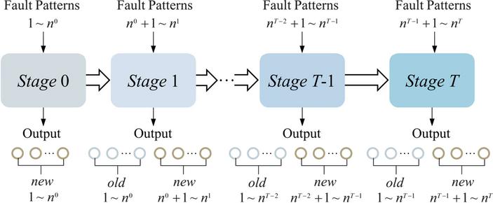
Figure 1 Overall training process for multi-fault diagnosis.

2.1 Dataset Construction

Ideally, the training dataset ${\mathcal{𝒟}}_{\mathrm{ideal}}^t$ for the incremental learning Stage $t(t=1,2,\mathrm{\dots },T)$ is

$${\mathcal{𝒟}}_{\mathrm{ideal}}^t=\{\underset{{\mathcal{\mathscr{H}}}_{\mathrm{ideal}}^t}{\underbrace{{\mathcal{𝒳}}^0,{\mathcal{𝒳}}^1,\mathrm{\dots },{\mathcal{𝒳}}^{t-1}}},{\mathcal{𝒳}}^t\}$$	(1)
$${\mathcal{𝒳}}^j={\{(x_i^j,y_i^j)\}}_{i=1}^{N^j},y_i^j\in {\mathcal{𝒴}}^j,j=0,1,\mathrm{\dots },T$$	(2)

where ${\mathcal{𝒳}}^0$ is the training dataset for the initial training, ${\mathcal{𝒳}}^1\sim {\mathcal{𝒳}}^T$ is the newly collected dataset from the incremental Stage 1 to Stage T, respectively, $x_i^j$ and $y_i^j$ are training samples and true labels, respectively, ${\mathcal{𝒴}}^j$ is the label space, if $j\ne j^{\prime }$, then ${\mathcal{𝒴}}^j\cap {\mathcal{𝒴}}^{j^{\prime }}=\mathrm{\varnothing }$, meaning that new fault patterns introduced to each stage are distinct and non-repetitive, $N^j$ is the number of training samples contained in ${\mathcal{𝒳}}^j$. $N^j$ is enough large so that the fault diagnosis model has adequate historical and new training samples to learn both the old and the new fault patterns. For the incremental learning Stage t, ${\mathcal{𝒳}}^0\sim {\mathcal{𝒳}}^{t-1}$ forms the ideal historical dataset ${\mathcal{\mathscr{H}}}_{\mathrm{ideal}}^t$, and ${\mathcal{𝒳}}^t$ is the newly collected dataset only containing new fault patterns emerging at Stage t.

However, due to limited storage resources and data privacy, not all the historical data can be recorded in practice. Therefore, the real-world training dataset ${\mathcal{𝒟}}_{\mathrm{real}}^t$ at the Stage t is revised as

$${\mathcal{𝒟}}_{\mathrm{real}}^t={\mathcal{\mathscr{H}}}_{\mathrm{real}}^t\cup {\mathcal{𝒳}}^t$$	(3)
$${\mathcal{\mathscr{H}}}_{\mathrm{real}}^t={\mathcal{\mathscr{H}}}_{\mathrm{real}}^{t-1}\cup ({\mathcal{𝒳}}_{\mathrm{sub}}^{t-1}\sim \mathcal{𝒫}({\mathcal{𝒳}}^{t-1},\alpha )),{𝔼}_{\mathcal{𝒫}}(|{\mathcal{𝒳}}_{\mathrm{sub}}^{t-1}|)=\alpha N^{t-1}$$	(4)

where ${\mathcal{\mathscr{H}}}_{\mathrm{real}}^0=\mathrm{\varnothing },\alpha \in [0,1)$ is a storage ratio on the historical dataset. Actually, $\alpha$ is a negligible value close to or equal to 0, and $\alpha =0$ indicates that the fault diagnosis model at the Stage t is trained solely on newly collected data. According to (3) and (4), a small subset of exemplars ${\mathcal{𝒳}}_{\mathrm{sub}}^{t-1}$ is randomly selected from the historical dataset in a storage ratio of $\alpha$ while newly collected data is continuously incorporated to construct the real-world training dataset for the Stage t.

2.2 Model Architecture

Denote ${\mathcal{ℳ}}^t$ as the fault diagnosis model consisting of a feature extractor ${\mathcal{ℱ}}^t$ with L intermediate layers $\{f_i^t;i=1,2,\mathrm{\dots },L\}$ and a classifier ${\mathcal{𝒞}}^t$ at the incremental Stage t [22]

$${\mathit{h}}_i^t=f_i^t\circ \mathrm{\cdots }\circ f_2^t\circ f_1^t(x)$$	(5)
$${\widehat{\mathit{y}}}^t={\mathcal{ℳ}}^t(x)={\mathcal{𝒞}}^t({\mathcal{ℱ}}^t(x))={\mathcal{𝒞}}^t(h_L^t)$$	(6)

where $\circ$ denotes function composition, ${\mathit{h}}_i^t\in {ℝ}^{d_i}$ is the i-th intermediate-layer representations, ${\widehat{\mathit{y}}}^t\in {ℝ}^{n^t}$ is the output-layer logits, $n^t$ is the number of the observed fault patterns until the Stage t.

In this article, a one-dimensional convolution neural network (1D-CNN), mainly composed of convolution modules (Conv), batch normalization, activation function, and a two-layer fully connected network (FCN), is employed as the fault diagnosis model. As shown in Figure 2, all the convolution modules form the feature extractor ${\mathcal{ℱ}}^t$, and the two-layer FCN forms the classifier ${\mathcal{𝒞}}^t$. Notably, the detailed architecture of the feature extractor, i.e., the number and the size of the convolution kernels, the convolution strides, and the paddings, remains the same during the incremental learning process. The number of nodes in the input layer of the classifier is unchanged as well, while nodes for new fault patterns are progressively added to the output layer.

2.3 Dual-aligned Knowledge Distillation Loss Design

At the incremental learning Stage t, the fault diagnosis model ${\mathcal{ℳ}}^t$ is expected to learn new fault patterns and maintain the capability to diagnose fault patterns learned from Stage 0 to Stage $t-1$. Generally, given the training dataset ${\mathcal{𝒟}}_{\mathrm{real}}^t$, the common loss is designed as

$${\mathcal{ℒ}}_{\mathrm{H}}^t(y,{\widehat{\mathit{y}}}^t;x)=-\sum _{i=1}^{n^t}\mathcal{ℐ}{(y)}_i\log \frac{\exp ({\widehat{y}}_i^t)}{{\sum }_j\exp ({\widehat{y}}_j^t)}$$	(7)
$$\mathcal{ℐ}(y)=[\mathcal{ℐ}{(y)}_1,\mathcal{ℐ}{(y)}_2,\mathrm{\dots },\mathcal{ℐ}{(y)}_i,\mathrm{\dots },\mathcal{ℐ}{(y)}_{n^t}]$$	(8)
$$\mathcal{ℐ}{(y)}_i=\{\begin{array}{cc}1,\hfill & i=y\hfill \\ 0,\hfill & i\ne y\hfill \end{array},i=1,2,\mathrm{\dots },n^t$$	(11)

where $\mathcal{ℐ}(\cdot )$ maps the true label y to a one-hot vector, $\mathcal{ℐ}{(y)}_i$ is the i-th item in the one-hot vector, and ${\widehat{y}}_i^t$ is the i-th logit in ${\widehat{\mathit{y}}}^t$.

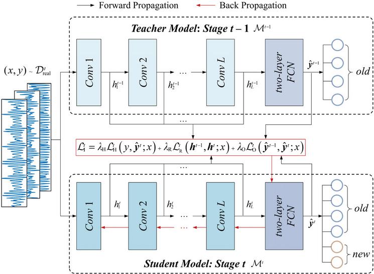
Figure 2 Class-incremental learning based on dual-aligned knowledge distillation for multi-fault diagnosis.

Simply optimizing (7) enables ${\mathcal{ℳ}}^t$ to achieve good fault diagnosis performance on new fault patterns but cannot guarantee comparable performance on old fault patterns, probably leading to catastrophic forgetting. Following the teacher-student paradigm of knowledge distillation proposed by Hinton [19], the fault diagnosis model ${\mathcal{ℳ}}^{t-1}$ which has been well-trained at Stage $t-1$, serves as the teacher model, and ${\mathcal{ℳ}}^t$ established by adding new nodes at the output layer of the teacher model serves as the student model. As shown in Figure 2, the knowledge of the teacher model, i.e., the diagnostic capability for old fault patterns, is transferred to the student model by dual-aligning the output-layer logits and the intermediate-layer representations accordingly.

The loss based on output-layer logits is designed as

$${\mathcal{ℒ}}_{\mathrm{O}}^t({\widehat{\mathit{y}}}^{t-1},{\widehat{\mathit{y}}}^t;x)={\epsilon }^2\sum _{i=1}^{n^{t-1}}{\tilde{y}}_i^{t-1}\log \frac{{\tilde{y}}_i^{t-1}}{{\tilde{y}}_i^t}$$	(12)
$${\tilde{y}}_i^{t-1}=\frac{\exp ({\widehat{y}}_i^{t-1}/\epsilon )}{{\sum }_j\exp ({\widehat{y}}_j^{t-1}/\epsilon )},{\tilde{y}}_i^t=\frac{\exp ({\widehat{y}}_i^t/\epsilon )}{\sum j\exp ({\widehat{y}}_j^t/\epsilon )}$$	(13)

where $\epsilon$ is a temperature factor to adjust the softness of the output logits distribution.

To further preserve the fault diagnosis performance on previously learned fault patterns, the loss based on intermediate-layer representations that encode discriminative fault features is further introduced

${\mathcal{ℒ}}_{\mathrm{R}}^t({\mathit{h}}^{t-1},{\mathit{h}}^t;x)$	$={\displaystyle \sum _{i=1}^L}{\omega }_i(1-\cos ({\mathit{h}}_i^{t-1},{\mathit{h}}_i^t))$
	$={\displaystyle \sum _{i=1}^L}{\omega }_i\left(1-{\displaystyle \frac{{\mathit{h}}_i^{t-1}\cdot {\mathit{h}}_i^t}{{\Vert {\mathit{h}}_i^{t-1}\Vert }_2{\Vert {\mathit{h}}_i^{t-1}\Vert }_2}}\right)$	(14)

where $\cos (\cdot )$ denotes cosine similarity, ${\omega }_i$ is a weight to adjust the importance of the i-th intermediate-layer feature representations, and ${\omega }_i\propto i$, i.e., representations encoding higher-level features in the deeper intermediate layer are given more importance.

Therefore, the total knowledge distillation loss is designed as

$${\mathcal{ℒ}}_{\mathrm{I}}^t(y,{\widehat{\mathit{y}}}^{t-1},{\mathit{h}}^{t-1},{\widehat{\mathit{y}}}^t,{\mathit{h}}^t;x)={\lambda }_{\mathrm{H}}{\mathcal{ℒ}}_{\mathrm{H}}^t+{\lambda }_{\mathrm{R}}{\mathcal{ℒ}}_{{}_{\mathrm{R}}}^t+{\lambda }_{\mathrm{O}}{\mathcal{ℒ}}_{\mathrm{O}}^t,(x,y)\sim {\mathcal{𝒟}}_{\mathrm{real}}^t$$

(15)

where ${\lambda }_{\mathrm{H}}$, ${\lambda }_{\mathrm{R}}$, and ${\lambda }_{\mathrm{O}}$ are hyper-parameters that balance the contributions of the three types of loss. By optimizing (15) with appropriate hyper-parameters, the fault diagnosis model can effectively retain diagnostic performance on old fault patterns while learning new fault patterns.

2.4 Class-incremental Learning Framework

The overall class-incremental learning framework includes initial training at Stage 0 and class-incremental learning from Stage 1 to Stage T, detailed in Algorithm 1.

At Stage 0, the fault diagnosis model ${\mathcal{ℳ}}^0$ is optimized according to (16) and (17).

$${\mathcal{ℒ}}_{\mathrm{H}}^0(y,{\widehat{\mathit{y}}}^0;x)=-\sum _{i=1}^{n^0}\mathcal{ℐ}{(y)}_i\log \frac{\exp ({\widehat{y}}_i^0)}{{\sum }_j\exp ({\widehat{y}}_j^0)},(x,y)\sim {\mathcal{𝒳}}^0$$	(16)
$$\underset{{\mathcal{ℳ}}^0}{\arg \min }{\mathcal{ℒ}}_{\mathrm{H}}^0(y,{\widehat{\mathit{y}}}^0;x)$$	(17)

From Stage 1 to Stage T, the fault diagnosis model ${\mathcal{ℳ}}^t(\text{t}=1,2,\mathrm{\dots },\text{T})$ is optimized according to (7)$\sim$(15) and (18)

$$\underset{{\mathcal{ℳ}}^t}{\arg \min }{\mathcal{ℒ}}_{\mathrm{I}}^t(y,{\widehat{\mathit{y}}}^{t-1},{\mathit{h}}^{t-1},{\widehat{\mathit{y}}}^t,{\mathit{h}}^t;x),t=1,2,\mathrm{\dots },T$$

(18)

Algorithm 1 Class-incremental learning method based on knowledge distillation
Input:	Initial training dataset ${\{x_i^0,y_i^0\}}_{i=1}^{N^0}\sim {\mathcal{𝒳}}^0$, incremental stage T, storage ratio $\alpha$, the number of intermediate layers L, weights ${\omega }_i(i=1,2,\mathrm{\dots },L)$, temperature factor $\epsilon$, hyper-parameters ${\lambda }_{\mathrm{H}}$, ${\lambda }_{\mathrm{R}}$, and ${\lambda }_{\mathrm{O}}$, initial training epoch $E_0$, incremental learning epoch $E_1$, batch size B
1:	Initialize ${\mathcal{ℳ}}^0$ according to (5) and (6)
2:	Define $N=N^0$
3:	For $e=0,1,\mathrm{\dots },E_0$
4:	For $b=0,1,\mathrm{\dots },N/B-1$
5:	Calculate ${\mathcal{ℒ}}_{\mathrm{H}}^0$ according to (6) and (16)
6:	Optimize ${\mathcal{ℳ}}^0$ according to (17)
7:	End
8:	End
9:	For $t=1,2,\mathrm{\dots },T$
10:	Initialize ${\mathcal{ℳ}}^t$ according to (5) and (6)
11:	Collect ${\mathcal{𝒳}}^t$ and form ${\mathcal{𝒟}}_{\mathrm{real}}^t$ according to (3) and (4)
12:	Update $N=|{\mathcal{𝒟}}_{\mathrm{real}}^t|$
13:	For $e=0,1,\mathrm{\dots },E_1$
14:	For $b=0,1,\mathrm{\dots },N/B-1$
15:	Calculate ${\mathcal{ℒ}}_{\mathrm{I}}^t$ according to (7) to (15)
16:	Optimize ${\mathcal{ℳ}}^t$ according to (18)
17:	End
18:	End
19:	End
Output:	well-train ${\mathcal{ℳ}}^T$

3 Experiment and Result Analysis

3.1 Experimental Setting and Fault Injection

The test rig is shown in Figure 3(a). Specifically, the tested axial piston pump is HP5V45 with 9 slipper-piston components, operating under a rated displacement of 45 cm³/r, a rated rotation speed of 2700 rpm, and a rated discharge port pressure of 32 MPa. To monitor periodic vibrations of the tested axial piston pump, a triaxial integrated electronic piezoelectric accelerometer is mounted at the center of its backend cover. The sampling frequency is set at 20 kHz. To fit the dimension-halving of convolution operations and binary computing logic, as well as to comprehensively extract periodic fault features, every 1024 consecutive sampling points are considered as a training sample.

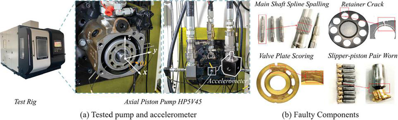
Figure 3 Experimental setup.

In addition to the normal state, four types of fault patterns shown in Figure 3(b), including main shaft spline spalling, retainer crack, valve plate scoring, and slipper-piston pair worn, are injected into the tested axial piston pump by replacing the normal components, respectively. Their time-domain vibration signals are depicted in Figure 4.

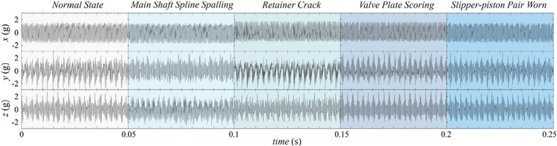
Figure 4 Time-domain vibration signals of normal state and 4 fault patterns.

For simulating a single fault occurring at different stages, the fault injection sequence and corresponding dataset description for the proposed method are detailed in Table 1. For simulating concurrent faults, the corresponding fault injection sequence and dataset description are listed in Table 2.

3.2 Comparison Experiment with Other Methods

The detailed architecture of the base model, i.e., the fault diagnosis model at Stage 0, is illustrated in Table 3. Model parameters in this architecture follow the established 1D-CNN designed for time series input [23]. The input size of Conv 1 is determined by the number of channels and the length of the input sample. The output size of FCN is determined by the number of fault patterns at the current stage. The activation function is LeakyReLU. As mentioned in Section 2.2, the architecture of Conv 1 $\sim$ Conv 4 remains the same during the whole training stages, while the number of output nodes in FCN increases progressively according to Table 1 or Table 2.

Table 1 Fault injection sequence and dataset description for single fault simulation

		Number of Training
		Samples	Number
		$\alpha =0.005$	$\alpha =0.01$	of Testing
Stage	Injected Patterns	New	Old	New	Old	New	Old	Label
0	Normal State	1728	0	1728	0	192	0	1
	Main Shaft Spline Spalling							2
1	Retainer Crack	864	8	864	17	96	192	3
2	Valve Plate Scoring	864	12	864	25	96	288	4
3	Slipper-piston Pair Worn	864	16	864	33	96	384	5
Note: During the initial training and incremental learning process, labels are mapped into one-hot vectors according to (8) and (11).

Table 2 Fault injection sequence and dataset description for concurrent faults simulation

		Number of Training
		Samples	Number
		$\alpha =0.005$	$\alpha =0.01$	of Testing
Stage	Injected Patterns	New	Old	New	Old	New	Old	Label
0	Normal State	2592	0	2592	0	288	0	1
	Main Shaft Spline Spalling							2
	Retainer Crack							3
1	Valve Plate Scoring	1728	12	1728	25	192	288	4
	Slipper-piston Pair Worn							5

Table 3 Detailed architecture of base model

Layer	Kernel Size/Strides	Kernel Number	Input	Output	Padding
Conv 1	64$\times$1/4$\times$1	4	3$\times$1024	4$\times$256	31
Conv 2	4$\times$1/2$\times$1	4	4$\times$256	4$\times$128	1
Conv 3	4$\times$1/2$\times$1	4	4$\times$128	4$\times$64	1
Conv 4	4$\times$1/2$\times$1	4	4$\times$64	4$\times$32	1
FCN	/	/	128	–	/
Note: For single fault, the number of output nodes in FCN of the base model is 2. For concurrent faults, the number of output nodes in FCN of the base model is 3.

For initial training at Stage 0, the optimizer is SGD with a momentum of 0.9 and a weight decay of 10^-4. Its parameters are selected based on empirical experience. The learning rate is 10^-3, the max training epoch is 20, and the batch size is 48. For class-incremental training from Stage 1, the proposed method is compared with LwF and fine-tuning. The optimizer of the proposed method is Adam, since it can adaptively adjust learning rate according to momentum and gradient, which helps to maintain the stability of model parameters related to old fault patterns. The batch size is 48, the learning rate is 10^-2, the max training epoch is 150, the temperature factor is 10, $[{\omega }_1,{\omega }_2,{\omega }_3,{\omega }_4]=[0.05,0.05,0.2,0.7]$ and $[{\lambda }_{\mathrm{H}},{\lambda }_{\mathrm{R}},{\lambda }_{\mathrm{O}}]=[0.5,1,0.5]$. For LwF, the optimizer is Adam, the batch size is 48, the warm-up rate is 10^-6 and the warm-up epoch is 400, the learning rate is 10^-4, and the max training epoch is 200. For fine-tuning, the optimizer is Adam, the batch size is 48, the learning rate is 10^-2, and the max training epoch is 150. These training settings are manually configured based on trial-and-error tuning to ensure that all the methods are trained to converge and reach a training accuracy of 100% for fair comparison.

To evaluate the effectiveness of each method, three performance metrics are defined as follows

${\mathcal{𝒜}}_{\mathrm{old}}^i$	$={\displaystyle \frac{C_{\mathrm{old}}^i}{N_{\mathrm{old}}^i}}\times 100\%$	(19)
${\mathcal{𝒜}}_{\mathrm{new}}^i$	$={\displaystyle \frac{C_{\mathrm{new}}^i}{N_{\mathrm{new}}^i}}\times 100\%$	(20)
${\mathcal{𝒜}}_{\mathrm{avg}}^i$	$={\displaystyle \frac{C_{\mathrm{new}}^i+C_{\mathrm{old}}^i}{N_{\mathrm{new}}^i+N_{\mathrm{old}}^i}}\times 100\%$	(21)

where $C_{\mathrm{old}}^i$ and $C_{\mathrm{new}}^i$ are the number of correctly diagnosed testing samples of old fault patterns and new fault patterns at Stage i, respectively, $N_{\mathrm{old}}^i$ and $N_{\mathrm{new}}^i$ are the number of testing samples of old fault patterns and new fault patterns at Stage i, respectively, ${\mathcal{𝒜}}_{\mathrm{old}}^i$ indicates the fault diagnosis performance on old fault patterns at Stage i, ${\mathcal{𝒜}}_{\mathrm{new}}^i$ indicates the fault diagnosis performance on new fault patterns at Stage i, and ${\mathcal{𝒜}}_{\mathrm{avg}}^i$ indicates the comprehensive fault diagnosis performance on all fault patterns at Stage i. All the methods are trained to converge. The training process is repeated 5 times, and the average performance metrics are considered as the fault diagnosis performance.

3.2.1 Comparison results for single fault simulation

The comparison results for single fault are listed in Table 4. For new fault patterns, all the methods demonstrate superior fault diagnosis performance at each stage, where the accuracy of LwF is slightly lower than 100%, and that of the proposed method and fine-tuning is 100%.

Table 4 Comparison experiment results (%) for single fault simulation

	Proposed Method	Proposed Method
Stage	($\alpha =0.005$)	($\alpha =0.01$)	LwF	Fine-tuning
0	${\mathcal{𝒜}}_{\mathrm{new}}^0$	100	100	100	100
	${\mathcal{𝒜}}_{\mathrm{avg}}^0$	100	100	100	100
1	${\mathcal{𝒜}}_{\mathrm{old}}^1$	55.10 $\pm$ 8.28	90.52 $\pm$ 11.57	12.08 $\pm$ 11.30	0
	${\mathcal{𝒜}}_{\mathrm{new}}^1$	100	100	99.58 $\pm$ 0.83	100
	${\mathcal{𝒜}}_{\mathrm{avg}}^1$	70.01 $\pm$ 5.52	93.08 $\pm$ 7.71	41.25 $\pm$ 7.58	33.33
2	${\mathcal{𝒜}}_{\mathrm{old}}^2$	37.01 $\pm$ 14.04	69.44 $\pm$ 11.02	7.57 $\pm$ 3.52	0
	${\mathcal{𝒜}}_{\mathrm{new}}^2$	100	100	97.08 $\pm$ 1.38	100
	${\mathcal{𝒜}}_{\mathrm{avg}}^2$	52.76 $\pm$ 10.53	77.08 $\pm$ 8.27	29.95 $\pm$ 2.67	25
3	${\mathcal{𝒜}}_{\mathrm{old}}^3$	37.86 $\pm$ 7.03	69.06 $\pm$ 4.25	6.56 $\pm$ 5.53	0
	${\mathcal{𝒜}}_{\mathrm{new}}^3$	100	100	97.08 $\pm$ 1.21	100
	${\mathcal{𝒜}}_{\mathrm{avg}}^3$	50.29 $\pm$ 5.62	75.25 $\pm$ 3.40	24.67 $\pm$ 4.53	20

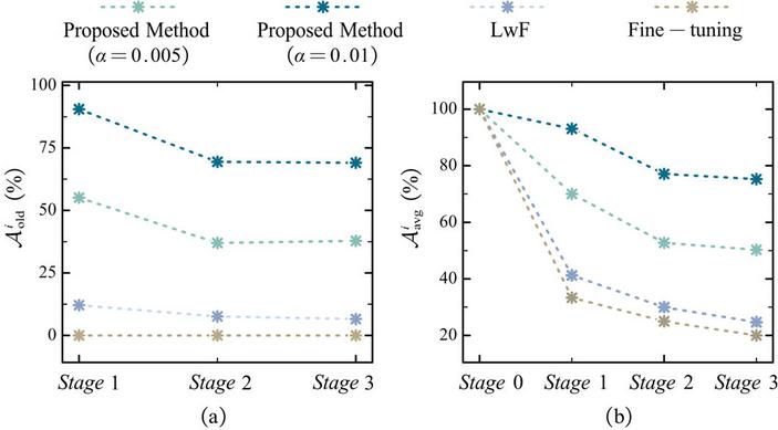
Figure 5 Comparison regarding ${\mathcal{𝒜}}_{\mathrm{old}}^i$ and ${\mathcal{𝒜}}_{\mathrm{avg}}^i$ for single fault simulation.

In contrast, for old fault patterns, all the methods suffer from different degrees of decline in accuracy, as shown in the Figure 5. Particularly, the accuracy of fine-tuning drops directly to 0% at each stage, indicating its poor ability in maintaining fault diagnosis performance on old fault patterns. LwF outperforms fine-tuning, with an accuracy of 6.56 $\pm$ 5.53% on old fault patterns and 24.67 $\pm$ 4.53% on all fault patterns at Stage 3. Given a small storage ratio, the proposed method surpasses LwF and fine-tuning. As the storage ratio increases from 0.005 to 0.01, the accuracy of the proposed method on old fault patterns and all fault patterns increases by 31.20% and 24.96%, respectively, at Stage 3. This highlights the significance of leveraging historical data in the incremental training process.

Table 5 Recalls of injected patterns at Stage 3(%) for single fault simulation

	Proposed Method	Proposed Method
Recall	($\alpha =0.005$)	($\alpha =0.01$)	LwF	Fine-tuning
${\mathcal{ℛ}}^1$	3.62	32.79	0	0
${\mathcal{ℛ}}^2$	68.04	84	0	0
${\mathcal{ℛ}}^3$	16.17	90.67	4.46	0
${\mathcal{ℛ}}^4$	62.04	75.71	21.13	0
${\mathcal{ℛ}}^5$	100	100	95.50	100

Furthermore, the recalls are calculated at Stage 3 to analyse the degradation of the fault diagnosis performance for each fault pattern

$${\mathcal{ℛ}}^i=\frac{C^i}{N^i}\times 100\%,i=1,2,3,4,5$$

(22)

where $N^1$, $N^2$, $N^3$, $N^4$, and $N^5$ are the number of testing samples of the normal state, main shaft spline spalling, retainer crack, valve plate scoring, and slipper-piston pair worn at Stage 3, respectively, $C^1$, $C^2$, $C^3$, $C^4$, and $C^5$ are the correctly diagnosed testing samples of the normal state, main shaft spline spalling, retainer crack, valve plate scoring, and slipper-piston pair worn at Stage 3, respectively, ${\mathcal{ℛ}}^1$, ${\mathcal{ℛ}}^2$, ${\mathcal{ℛ}}^3$, ${\mathcal{ℛ}}^4$, and ${\mathcal{ℛ}}^5$ are the recall of the normal state, main shaft spline spalling, retainer crack, valve plate scoring, and slipper-piston pair worn at Stage 3, respectively. ${\mathcal{ℛ}}^i$ indicates fault diagnosis performance on each fault pattern at Stage 3. The average recalls at Stage 3 are listed in Table 5 and visualized in Figure 6. The results generally demonstrate a common trend among all the methods, i.e., as the incremental learning progresses, fault diagnosis performance degrades more severely on older fault patterns compared to new ones, suggesting the catastrophic forgetting phenomenon. However, two exceptions are observed in the proposed method, i.e., ${\mathcal{ℛ}}^2$ exceeds ${\mathcal{ℛ}}^3$ and ${\mathcal{ℛ}}^4$ at a storage ratio of 0.005, and ${\mathcal{ℛ}}^4$ falls below both ${\mathcal{ℛ}}^2$ and ${\mathcal{ℛ}}^3$ at a storage ratio of 0.01.

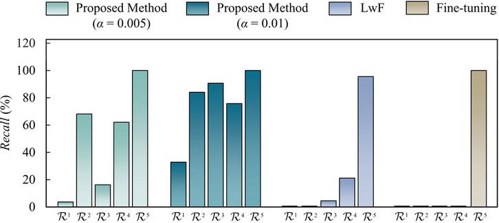
Figure 6 Recalls of injected patterns at Stage 3 for single fault simulation.

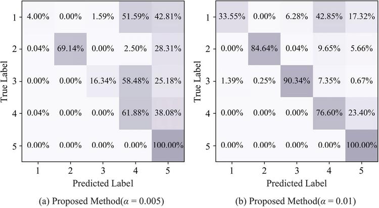
Figure 7 Confusion matrixes at Stage 3 for single fault simulation (1: normal state, 2: main shaft spline spalling, 3: retainer crack, 4: valve plate scoring, 5: slipper-piston pair worn).

To analyze detailed degrees of forgetting and retention across different fault patterns, the confusion matrixes at Stage 3 for single fault simulation are drawn Figure 7. Given the storage ratio of 0.005, the main shaft spline spalling and the valve plate scoring are mainly misclassified as the slipper-piston pair worn. Moreover, the retainer crack exhibits higher misclassification rate as the valve plate scoring (58.48%) than as the slipper-piston pair worn (25.18%), which indicates that the fault features of the retainer crack tend to be obscured by those of the valve plate scoring. With the storage ratio increasing, though the retainer crack is still misclassified as the valve plate scoring, its misclassification rate is greatly reduced thanks to more training data. Notably, given the storage ratio of 0.01, the valve plate scoring remains more susceptible to misclassification as the slipper-piston pair worn compared with other old fault patterns. Overall, the diagnosis performance of all old fault patterns has degraded, yet the degrees of forgetting and retention vary across different fault patterns.

3.2.2 Comparison results for concurrent faults simulation

The comparison results for concurrent faults are listed in Table 6. Similarly, all the methods ensure good fault diagnosis capability on new fault patterns. While for old fault patterns, the most severe degradation of accuracy is still observed in Fine-tuning, dropping directly to 1.46 $\pm$ 0.40%. The fault diagnosis performance on old fault patterns of LwF is slightly better than Fine-tuning by 12.85%, thanks to its output-logits alignment. With a storage ratio of 0.005 and 0.01, the proposed method outperforms LwF by 39.09% and 56.73% on old fault patterns, respectively, indicating its effectiveness in incremental learning for concurrent faults.

Table 6 Comparison experiment results (%) for concurrent faults simulation

		Proposed Method	Proposed Method
Stage	($\alpha =0.005$)	($\alpha =0.01$)	LwF	Fine-tuning
0	${\mathcal{𝒜}}_{\mathrm{new}}^0$	100	100	100	100
	${\mathcal{𝒜}}_{\mathrm{avg}}^0$	100	100	100	100
1	${\mathcal{𝒜}}_{\mathrm{old}}^1$	53.40 $\pm$ 11.69	71.04 $\pm$ 12.00	14.31 $\pm$ 8.45	1.46 $\pm$ 0.40
	${\mathcal{𝒜}}_{\mathrm{new}}^1$	100	100	94.38 $\pm$ 10.74	100
	${\mathcal{𝒜}}_{\mathrm{avg}}^1$	72.04 $\pm$ 7.01	82.63 $\pm$ 7.20	46.33 $\pm$ 5.73	40.88 $\pm$ 0.24

Table 7 Recalls of injected patterns at Stage 1(%) for concurrent faults simulation

		Proposed Method	Proposed Method
Recall	($\alpha =0.005$)	($\alpha =0.01$)	LwF	Fine-tuning
${\mathcal{ℛ}}^1$	0.38	47.04	29.54	5.38
${\mathcal{ℛ}}^2$	71.92	91.83	1.46	0
${\mathcal{ℛ}}^3$	83.79	69.46	14.54	0
${\mathcal{ℛ}}^4$	100	100	93.25	100
${\mathcal{ℛ}}^5$	100	100	93.83	100

Also, the recalls regarding each fault at final stage are illustrated in Table 7 and Figure 8. Obviously, recalls of old fault patterns, i.e., ${\mathcal{ℛ}}^1$, ${\mathcal{ℛ}}^2$, and ${\mathcal{ℛ}}^3$, exhibits different degrees of degradation across different methods. Both the LwF and Fine-tuning show better recall on normal state than main shaft spline spalling fault and retainer crack. In contrast, for the proposed method, the recall of the normal state is the lowest, achieving only 0.38% at a storage ratio of 0.005 and 47.04% at a storage ratio of 0.01, respectively.

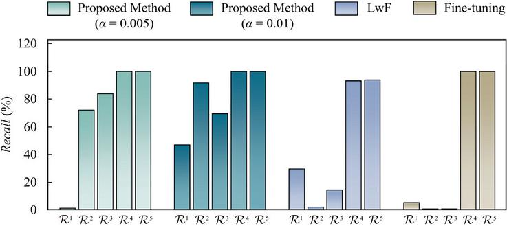
Figure 8 Recalls of injected patterns at Stage 1 for concurrent faults simulation.

3.3 Ablation Experiment of the Proposed Method

To verify the contribution of each type of loss in (15), the ablation experiment is conducted regarding single fault simulation. Specifically, Ablation 1 sets $[{\lambda }_{\mathrm{H}},{\lambda }_{\mathrm{R}},{\lambda }_{\mathrm{O}}]=[1,0,0]$ and Ablation 2 sets $[{\lambda }_{\mathrm{H}},{\lambda }_{\mathrm{R}},{\lambda }_{\mathrm{O}}]=[0.5,0,0.5]$. Other training settings are consistent with those described in Section 3.2. The ablation experiment results are listed in Table 8, and results regarding ${\mathcal{𝒜}}_{\mathrm{old}}^i$ and ${\mathcal{𝒜}}_{\mathrm{avg}}^i$ are drawn in Figure 9.

Table 8 Ablation experiment results (%)

	$\alpha =0.005$			$\alpha =0.01$
			Proposed			Proposed
Stage	Ablation 1	Ablation 2	Method	Ablation 1	Ablation 2	Method
0	${\mathcal{𝒜}}_{\mathrm{new}}^0$	100	100	100	100	100	100
	${\mathcal{𝒜}}_{\mathrm{avg}}^0$	100	100	100	100	100	100
1	${\mathcal{𝒜}}_{\mathrm{old}}^1$	35.42 $\pm$ 21.49	46.98 $\pm$ 10.62	55.10 $\pm$ 8.28	71.25 $\pm$ 16.25	81.87 $\pm$ 13.78	90.52 $\pm$ 11.57
	${\mathcal{𝒜}}_{\mathrm{new}}^1$	100	100	100	100	100	100
	${\mathcal{𝒜}}_{\mathrm{avg}}^1$	56.94 $\pm$ 14.33	64.65 $\pm$ 7.08	70.01 $\pm$ 5.52	80.83 $\pm$ 10.84	87.92 $\pm$ 9.18	93.08 $\pm$ 7.71
2	${\mathcal{𝒜}}_{\mathrm{old}}^2$	28.40 $\pm$ 11.48	46.74 $\pm$ 8.35	37.01 $\pm$ 14.04	69.72 $\pm$ 8.51	75.90 $\pm$ 9.75	69.44 $\pm$ 11.02
	${\mathcal{𝒜}}_{\mathrm{new}}^2$	100	100	100	100	100	100
	${\mathcal{𝒜}}_{\mathrm{avg}}^2$	46.30 $\pm$ 8.61	60.05 $\pm$ 6.26	52.76 $\pm$ 10.53	77.29 $\pm$ 6.39	81.93 $\pm$ 7.31	77.08 $\pm$ 8.27
3	${\mathcal{𝒜}}_{\mathrm{old}}^3$	22.76 $\pm$ 8.97	31.77 $\pm$ 4.29	37.86 $\pm$ 7.03	65.10 $\pm$ 3.40	66.04 $\pm$ 6.78	69.06 $\pm$ 4.25
	${\mathcal{𝒜}}_{\mathrm{new}}^3$	100	100	100	100	100	100
	${\mathcal{𝒜}}_{\mathrm{avg}}^3$	38.21 $\pm$ 7.18	45.42 $\pm$ 3.43	50.29 $\pm$ 5.62	72.08 $\pm$ 2.72	72.83 $\pm$ 5.42	75.25 $\pm$ 3.40

Similarly, all the methods achieve an accuracy of 100% on new fault patterns and generally degrade on old fault patterns during the incremental training process. At a storage ratio of 0.005, ablation 2 and the proposed method always outperform ablation 1, indicating that aligning the output-logits and intermediate-representations enhances the capability to preserve fault diagnosis performance on old fault patterns. According to Figure 9(a) and 9(c), the proposed method performs worse than Ablation 2 on old fault patterns at Stage 2. However, from Stage 2 to Stage 3, the accuracy of Ablation 2 on old fault patterns decreases by 9.86% and 14.97%, at a storage ratio of 0.01 and 0.005, respectively. While that of the proposed method only decreases by 0.38% at a storage ratio of 0.01, and even increases by 0.85% at a storage ratio of 0.005. This indicates that, compared to relying solely on output-layer logits, dual alignment of both output-layer logits and the intermediate-layer representations further improves the ability to retain fault diagnosis performance on old fault patterns.

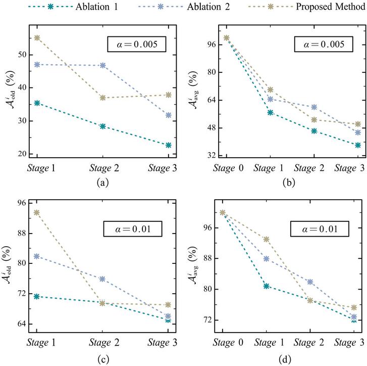
Figure 9 Ablation regarding ${\mathcal{𝒜}}_{\mathrm{old}}^i$ and ${\mathcal{𝒜}}_{\mathrm{avg}}^i$.

3.4 Analysis of Temperature Factor

The temperature factor $\epsilon$ is a crucial hyper-parameter in knowledge distillation, which control the softness of the output logits distribution, i.e., higher the temperature factor, softer the output logits distribution. Therefore, the impact of different temperature factor is analyzed regarding concurrent faults with a storage ratio of 0.005.

As shown in Table 9 and Figure 10, the proposed method performs the worst at a temperature factor of 1, whose average testing accuracy of old fault patterns only achieves 32.22 $\pm$ 18.61%. This is because the output logits approach hard labels at a temperature factor of 1, preventing the student from learning how the teacher learns and generalizes on old fault patterns. As the temperature factor increases, the proposed method generally exhibits better fault diagnosis performance on old fault patterns, with accuracy of 52.57 $\pm$ 8.54% ($\epsilon =2$), 51.88 $\pm$ 14.92% ($\epsilon =5$), and 53.40 $\pm$ 11.69% ($\epsilon =10$), respectively. However, from a temperature factor of 15, the fault diagnosis performance on old fault patterns degrades due to the over-softened logits distribution. Therefore, either excessively low value or excessively high value of the temperature factor degrade the fault diagnosis performance on old fault patterns. According to Table 9, the results suggest that the proposed method performs better at an intermediate temperature factor ranging from 2 to 10.

Table 9 Fault diagnosis performance (%) of the proposed method with a storage ratio of 0.005 under different temperature factors

Stage		$\epsilon =1$	$\epsilon =2$	$\epsilon =5$	$\epsilon =10$	$\epsilon =15$	$\epsilon =20$
0	${\mathcal{𝒜}}_{\mathrm{new}}^0$	100	100	100	100	100	100
	${\mathcal{𝒜}}_{\mathrm{avg}}^0$	100	100	100	100	100	100
1	${\mathcal{𝒜}}_{\mathrm{old}}^1$	32.22 $\pm$ 18.61	52.57 $\pm$ 8.54	51.88 $\pm$ 14.92	53.40 $\pm$ 11.69	50.07 $\pm$ 7.54	42.57 $\pm$ 7.69
	${\mathcal{𝒜}}_{\mathrm{new}}^1$	100	100	100	100	100	100
	${\mathcal{𝒜}}_{\mathrm{avg}}^1$	59.33 $\pm$ 11.17	71.54 $\pm$ 5.12	71.13 $\pm$ 8.95	72.04 $\pm$ 7.01	70.04 $\pm$ 4.53	65.54 $\pm$ 4.61

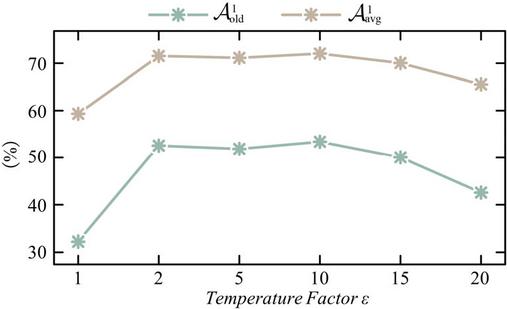
Figure 10 ${\mathcal{𝒜}}_{\mathrm{old}}^1$ and ${\mathcal{𝒜}}_{\mathrm{avg}}^1$ of the proposed method under different temperature factors.

4 Conclusions

For multi-fault diagnosis of the axial piston pump, a class-incremental learning method based on dual-aligned knowledge distillation is proposed to integrate newly emerging fault patterns as well as preserving fault diagnosis performance on old fault patterns. Comparison experiment with LwF and fine-tuning regarding single fault and concurrent faults are conducted, and ablation experiment around each loss item are conducted to verify the effectiveness of the proposed method. Also, the impact of the temperature factor is analyzed. Main conclusions are drawn as follows.

(1) Storing only a small portion of historical data can greatly improve the fault diagnosis performance on old fault patterns.

(2) Dual alignment of the output-layer logits and the intermediate-layer representations further enhances knowledge preservation on old fault patterns.

(3) The proposed method yields optimal fault diagnosis performance at moderate temperature factors ($\epsilon =2\sim 10$).

The proposed method is not limited to the axial piston pump. Its core class-incremental learning and knowledge distillation mechanisms are also applicable to time-series signal-based fault diagnosis for other rotating machinery and hydraulic systems. However, there is still much room for improvement.

(1) In current framework, the weights for three loss terms are set as fixed value. During different training epochs, the contribution of each loss cannot be dynamically adjusted to match the demand of different incremental stages. Therefore, an adaptive weight strategy needs to be designed to balance the contribution of different loss terms.

(2) Historical exemplars are randomly selected, without considering their quality. Therefore, how to select exemplars that can represent the distributions of old fault patterns needs to be further discussed.

Acknowledgements

This work is supported by the National Science and Technology Major Project of the Ministry of Science and Technology of China (G24002).

References

[1] S. Mukherjee, L. Shang, A. Vacca, ‘Numerical analysis and experimental validation of the coupled thermal effects in swashplate type axial piston machines’, Mechanical Systems and Signal Processing, vol. 220, p. 111673, 2024.

[2] P. Michael, K. Stelson, D. Williams, H. Malik, ‘Dynamometer testing of hydraulic fluids in an axial piston pump under simulated backhoe loader trenching conditions’, Fluid Power Systems Technology, vol. V001T01A14, 2022.

[3] L.V. Larsson, P. Krus, ‘Modelling of the swash plate control actuator in an axial piston pump for a hardware-in-the-loop simulation test rig’, Fluid Power Systems Technology, vol. V001T01A44, 2016.

[4] I. Baus, R. Rahmfeld, A. Schumacher, H.C. Pedersen, ‘Systematic methodology for reliability analysis of components in axial piston units’, Fluid Power Systems Technology, vol. V001T01A9, 2019.

[5] N. Keller, A. Sciancalepore, A. Vacca, ‘Condition Monitoring of an Axial Piston Pump on a Mini Excavator’, International Journal of Fluid Power, vol. 24, no. 02, pp. 171–206, 2023.

[6] R. Ivantysyn, J. Weber, ‘Advancing Thermal Monitoring in Axial Piston Pumps: Simulation, Measurement, and Boundary Condition Analysis for Efficiency Enhancement’, International Journal of Fluid Power, pp. 547–590, 2024.

[7] S. Wang, J. Xiang, Y. Zhong, H. Tang, ‘A data indicator-based deep belief networks to detect multiple faults in axial piston pumps’, Mechanical Systems and Signal Processing, vol. 112, pp. 154–170, 2018.

[8] Y. He, H. Tang, Y. Ren, A. Kumar, ‘A semi-supervised fault diagnosis method for axial piston pump bearings based on DCGAN’, Measurement Science and Technology, vol. 32, no. 12, p. 125104, 2021.

[9] S. Wang, H. Shuai, J. Hu, et al., ‘Few-shot fault diagnosis of axial piston pump based on prior knowledge-embedded meta learning vision transformer under variable operating conditions’, Expert Systems with Applications, vol. 269, p. 126452, 2025.

[10] S. Liu, J. Zhang, W. Huang, F. Lyu, D. Wang, B. Xu, ‘Temporal–Spatial Attention Network: A Novel Axial Piston Pump Coupled Fault Diagnosis Method’, IEEE Transactions on Instrumentation and Measurement, vol. 73, pp. 1–15, 2024.

[11] E. Belouadah, A. Popescu, I. Kanellos, ‘A comprehensive study of class incremental learning algorithms for visual tasks’, Neural Networks, vol. 135, pp. 38–54, 2021.

[12] A.A. Rusu, N.C. Rabinowitz, G. Desjardins, et al., ‘Progressive neural networks’, arXiv preprint arXiv:1606.04671, 2016.

[13] Y.-X. Wang, D. Ramanan, M. Hebert, ‘Growing a brain: Fine-tuning by increasing model capacity’, Proc. IEEE Conf. on Computer Vision and Pattern Recognition, pp. 2471–2480, 2017.

[14] R. Aljundi, M. Lin, B. Goujaud, Y. Bengio, ‘Gradient based sample selection for online continual learning’, Advances in Neural Information Processing Systems, vol. 32, 2019.

[15] A. Odena, C. Olah, J. Shlens, ‘Conditional image synthesis with auxiliary classifier gans’, Int. Conf. on Machine Learning, pp. 2642–2651, 2017.

[16] J. Kirkpatrick, R. Pascanu, N. Rabinowitz, et. al., ‘Overcoming catastrophic forgetting in neural networks’, Proc. National Academy of Sciences, vol. 114, no. 13, pp. 3521–3526, 2017.

[17] Z. Li, D. Hoiem, ‘Learning without forgetting’, IEEE Trans. on Pattern Analysis and Machine Intelligence, vol. 40, no. 12, pp. 2935–2947, 2017.

[18] S.-A. Rebuffi, A. Kolesnikov, G. Sperl, C.H. Lampert, ‘iCaRL: Incremental classifier and representation learning’, Proc. IEEE Conf. on Computer Vision and Pattern Recognition, pp. 2001–2010, 2017.

[19] G. Hinton, O. Vinyals, J. Dean, ‘Distilling the Knowledge in a Neural Network’, arXiv preprint arXiv:1503.02531, 2015.

[20] G.M. Van de Ven, T. Tuytelaars, A.S. Tolias, ‘Three types of incremental learning’, Nature Machine Intelligence, vol. 4, no. 12, pp. 1185–1197, 2022.

[21] S. Yan, H. Shao, X. Wang, J. Wang, ‘Few-shot class-incremental learning for system-level fault diagnosis of wind turbine’, IEEE/ASME Trans. on Mechatronics, 2024.

[22] M. Kang, J. Park, B. Han, ‘Class-incremental learning by knowledge distillation with adaptive feature consolidation’, Proc. IEEE/CVF Conf. on Computer Vision and Pattern Recognition, pp. 16071–16080, 2022.

[23] M. Ji, G. Peng, S. Li, et al., ‘A neural network compression method based on knowledge-distillation and parameter quantization for the bearing fault diagnosis’, Applied Soft Computing, vol. 127, p. 109331, 2022.

Biographies

Dandan Wang received the B.S. degree in mechanical engineering from Zhejiang University, Hangzhou, China, in 2023. She is currently pursuing the Master’s degree in mechatronics engineering with the Department of Mechanical Engineering, Zhejiang University, Hangzhou, China. Her current research is focused on intelligent axial piston pumps, deep learning, fault diagnosis and prognosis.

Shihao Liu received the B.S. degree in mechatronics engineering from Zhejiang University, Hangzhou, China, in 2019. He is currently pursuing the Ph.D. degree in mechatronics engineering with the Department of Mechanical Engineering, Zhejiang University, Hangzhou, China. His current research is focused on intelligent axial piston pumps, deep learning, fault diagnosis, and prognosis.

Junhui Zhang received the Ph.D. degree in mechatronics engineering from Zhejiang University, Hangzhou, China, in 2012. He is currently an Associate professor with the State Key Laboratory of Fluid Power and Mechatronic Systems, Zhejing University. He has authored or co-authored more than 60 papers indexed by SCI and applied more than 30 National Invention Patents with granted. He is supported by the National Science Fund for Excellent Young Scholars. His research interests include high-speed hydraulic pumps/motors and hydraulic robots.

Fei Lyu received the Ph.D. degree in mechatronics engineering from Zhejiang University, Hangzhou, China, in 2022. He is currently a postdoc with the State Key Laboratory of Fluid Power and Mechatronic Systems, Zhejiang University. His research interests focus on tribological analysis and predictive maintenance of hydrostatic pumps and motors.

Weidi Huang received the Ph.D. degree in mechanical engineering from Zhejiang University, Hangzhou, China, in 2018. He is currently a research assistant with the State Key Laboratory of Fluid Power and Mechatronic Systems, Zhejiang University. His current research is focused on the dynamic modelling of axial piston pumps, condition monitoring, and fault diagnosis.

Bing Xu received the Ph.D. degree in fluid power transmission and control from Zhejiang University, Hangzhou, China, in 2001. He is currently a Professor and a Doctoral Tutor with the Institute of Mechatronic Control Engineering, and the Deputy Director of the State Key Laboratory of Fluid Power and Mechatronic Systems, Zhejiang University. He has authored or coauthored more than 200 journal and conference papers and authorized 49 patents. Dr. Xu is a Chair Professor of the Yangtze River Scholars Programme and a Science and Technology Innovation Leader of the Ten Thousand Talent Programme.

International Journal of Fluid Power, Vol. 27_1, 29–52
doi: 10.13052/ijfp1439-9776.2712
© 2026 River Publishers