Data-driven Adaptive Thresholding Model for Real-time Valve Delay Estimation in Digital Pump/Motors
Abdallah A. Chehade1, Farid Breidi2,*, Keith S. Pate3 and John Lumkes4
1University of Michigan-Dearborn 4901 Evergreen Rd. Dearborn, MI 48128, USA
2University of Southern Indiana 8600 University Blvd. Evansville, IN 47712, USA
3Allison Transmission One Allison Way Indianapolis, IN 46222, USA
4Purdue University 225 South University St. West Lafayette, IN 47907, USA
E-mail: Farid@Breidi.com
* Corresponding Author
Received 15 January 2019; Accepted 03 February 2020; Publication 07 March 2020
Abstract
Valve characteristics are an essential part of digital hydraulics. The on/off solenoid valves utilized on many of these systems can significantly affect the performance. Various factors can affect the speed of the valves causing them to experience various delays, which impact the overall performance of hydraulic systems. This work presents the development of an adaptive statistical based thresholding real-time valve delay model for digital Pump/Motors. The proposed method actively measures the valve delays in real-time and adapts the threshold of the system with the goal of improving the overall efficiency and performance of the system. This work builds on previous work by evaluating an alternative method used to detect valve delays in real-time. The method used here is a shift detection method for the pressure signals that utilizes domain knowledge and the system’s historical statistical behavior. This allows the model to be used over a large range of operating conditions, since the model can learn patterns and adapt to various operating conditions using domain knowledge and statistical behavior. A hydraulic circuit was built to measure the delay time experienced from the time the signal is sent to the valve to the time that the valve opens. Experiments were conducted on a three piston in-line digital pump/motor with 2 valves per cylinder, at low and high pressure ports, for a total of six valves. Two high frequency pressure transducers were used in this circuit to measure and analyze the differential pressure on the low and high pressure side of the on/off valves, as well as three in-cylinder pressure transducers. Data over 60 cycles was acquired to analyze the model against real time valve delays. The results show that the algorithm was successful in adapting the threshold for real time valve delays and accurately measuring the valve delays.
Keywords: Fluid power, digital hydraulics, digital pump motor, hydraulics, valve delay.
Introduction
Fluid Power is a technology which uses pressurized fluids to transmit and control power. These pressurized fluids store energy, which can be used to move and rotate components in mechanical systems. Fluid power systems are used in a variety of applications including automotive, mining, manufacturing, and aerospace.
In most applications, fluid power is used because of its ability to flexibly transfer energy and power over long distances. Another quality of fluid power systems is the relatively low maintenance required to upkeep the system. This is due to the lack of moving components used in the system, compared to mechanical and electrical systems.
Although fluid power is a relatively old technology, there are still new advancements and innovative methods being developed to enhance and modernize the field. Each advancement and modernization provides opportunity to advance how fluid power systems are and can be used. Fluid power has multiple areas that can be improved, with a main focus being on efficiency, compactness, and effectiveness (Stelson and Li, 2013). One specific area of study being closely analyzed is efficiency. Many existing fluid power systems use multiple components in series; all with various efficiencies. The individual efficiency of each of these components can largely effect the overall efficiency of fluid power systems.
At the heart of fluid power systems is the pump/motor, used to create flow for the hydraulic system. Under ideal conditions, pumps/motors can reach overall efficiencies higher than 90%, but can drop below 75% based on the running conditions of the pump (Love, 2014). Current state-of-the-art variable displacement pumps/motors can drop as low as 30% at low displacements, due to losses throughout the system which are not linearly dependent on displacement.
Another key component of many fluid power systems is valves used to control the system. The efficiency of the valves can depend on the type of valves and the amount used. Love (2009) reports that valves used in industry excavating equipment, can consume up to 43% of the energy of the system. This can substantially decrease the overall efficiency of the system. Thus there is motivation to replace certain valves of low efficiencies with alternative ones.
Recently, digital hydraulics has become more prominent in fluid power research. There has been an expanded focus on digital fluid power in the last decade due to the improved switching times and the use of robust components, increasing the desire for this new technology (Linjama, 2011). Digital hydraulics introduces the control of fluid power systems using multiple on/off solenoid valves to control pressure, flow and direction. It aims at offering efficiency improvements by reducing the amount of losses currently found in conventional units (Holland, 2012).
Background
Digital hydraulics is an emerging field which incorporates advanced controls, machine learning, and digital electronics in fluid power systems with the goal of improving performance, efficiency, energy savings, and overall productivity. Such improvements can be obtained by improving power management at a system level, like introducing hybrid configurations or displacement control, or at a component level like pumps, motors, or valves. With the emergence of digital fluid power technologies, unique pump/motor configurations could be attained by utilizing high flow and speed on/off valves. These digital pump/motor systems aim at improving the overall efficiency by discretizing the flow levels or pressures through the use of digital valves, maintaining a relatively high efficiency or a lower loss in input power over a wider range of displacement (Breidi et al., 2017).
A digital pump/motor unit utilizes on/off valves to vary the displacement of the unit, replacing the valve plate that was commonly used to port the hydraulic fluid. An in-line three-piston digital pump/motor configuration has been selected for this work, shown in Figure 1.
In-line piston units are commonly used for high pressure applications, with working pressures going up to 500 bar at a high efficiency (Ivantysyn & Ivantysynova, 1993/2003). Standard in-line units cannot vary their displacement, but with the introduction of on/off valves per displacement chamber, variable displacement could be achieved.
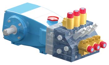
Figure 1 In-line digital pump/ motor assembly (Breidi et al., 2017).
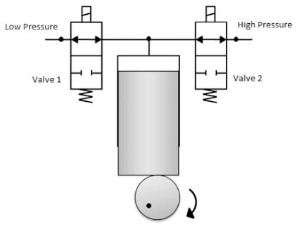
Figure 2 Digital pump/motor single piston valve configuration.
The unit of interest utilizes two high speed on/off valves for each individual displacement chamber, for a total of six valves; a single digital pump/motor piston valve configuration is shown in Figure 2. Such a configuration allows active and independent control of the displacement of each chamber, and to keep the pressure in the disabled chambers low (Breidi et al., 2015). Keeping the pressure low in the inactive pumping chambers scales down the leakage losses to be proportional with displacement, improving the efficiency as it eliminates the shear and leakage losses found on conventional pump/motors between the cylinder block and the valve plate, and reducing compressibility losses compared to conventional units (Holland, 2012).
By controlling the states of the valves at different shaft locations, pumping or motoring could be achieved, along with the ability to vary the displacement with the use of unique operating strategies. Several digital pump/motor operating strategies have been proposed in literature (Nieling et al., 2005) and four of them have been experimentally implemented, partial flow-diverting, partial flow-limiting, sequential flow-diverting, and sequential flow-limiting (Merrill et al., 2013). All the experiments and data presented in this paper were conducted using the partial flow-diverting operating strategy, so the interest of this paper, only this method will be described (others are described in Merrill, 2012).
Partial Flow-Diverting
Partial flow-diverting refers to the operating strategy where excess flow is diverted from the displacement chamber to the low pressure port, rather than delivering the flow through the high pressure port. Such a strategy enables changing the displacement from 100% to 0% by diverting any percentage of flow through the low pressure port. This strategy can be applied whether the unit is pumping or motoring. A 50% displacement pumping cycle is shown in Figure 3. Starting from the top-dead-center (TDC) and as the piston is moving down, flow would enter the chamber from the low pressure port through valve 1, while valve 2 is kept closed, until the piston reaches the bottom-dead-center (BDC) filling in the entire chamber with fluid, denoted by (1) on the figure. To achieve variable displacement, as the piston is moving back up, the same valve states would be kept (valve 1 would be kept open while valve 2 is closed). This allows part of the fluid to be diverted back through valve 1 to the low pressure port until the volume of fluid in the chamber is slightly larger than the desired displacement (50%) to allow for pre-compression, denoted by (2) on the figure. To achieve this, both valves are shut while the piston is moving up to compress the chamber fluid to the desired pressure, denoted by (3) on the figure. Once the chamber volume reaches the desired pressure, valve 2 opens and the pressurized fluid would be delivered to the high pressure port, denoted by (4) on the figure. Such a strategy can achieve any displacement percentage, but would be highly dependent on the valves opening areas and response times.
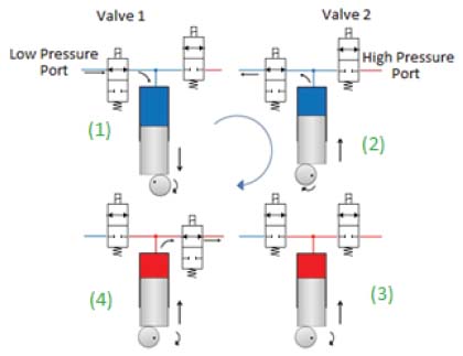
Figure 3 Partial flow-diverting pumping cycle, 50% displacement.
Significance of Valve Response Times
To investigate the significance of valve timing on the performance of digital pump/motors, Merrill et al. (2013) developed a multi-domain simulation model using MATLAB based Simscape. The simulation model was for a three and seven piston in-line pump.
The model was used to predict losses occurring through leakages, compressibility, friction, and metering. The simulation results concluded that a small delay in the valve opening or closing would result in major noise generation and energy losses. Figure 4 represents the losses resulting from the error in valve timing, simulated for a 7-piston in-line pump running at 3000 rpm, 300 bar, and 57% displacement in a partial flow-diverting operating strategy. Results show that if the valves were to open when expected, valve throttling losses, shown in red, were 6%. However, when a small error in valve opening of 2 milliseconds occurs, the losses significantly increase. This demonstrated the importance of valve timing in the viability of digital fluid power systems.
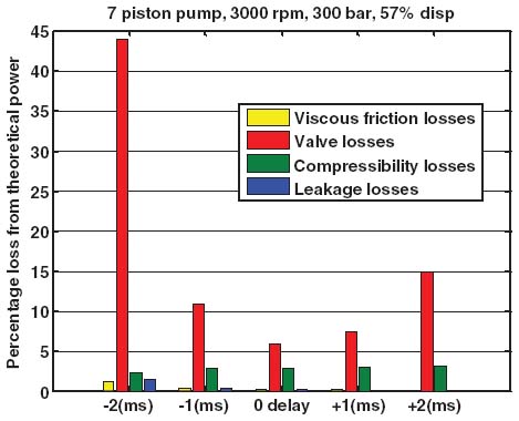
Figure 4 Percentage loss from theoretical power due to a delay in valve opening (Merrill et al., 2013).
To improve the response times of commercially available on/off valves, industry has been utilizing a peak-and-hold and reverse current solenoid driving strategies (Breidi et al., 2015). The peak-and-hold concept is based on speeding up the establishment of the magnetic field by using an initial high voltage signal for a short duration, overcoming the inductance and eddy current lag. This peak signal is then followed by a holding current which keeps the armature in place. Similarly, the reverse current strategy speeds up the decaying of the lingering current and residual magnetism in the solenoid, which opposes the closing force of the spring (Batdorff, 2010).
In order to reduce the losses due to the variation in the valve delays, Breidi et al. (2017) developed a real-time valve correction algorithm which uses the pressure ripples on the high and low pressure lines to actively detect the valve delay times. The concept was based on the knowledge that valve 1 is connected to the low pressure port, while valve 2 is connected to the high pressure port, as shown in Figure 2. So when a valve state changes, a pressure ripple is expected to appear at the respective port, corresponding to the time when the valve actually changed its state. Given that the sending time of the valve signal is known, the delay time of the valve corresponds to the difference in time between the valve signal and the peak appearance. The implemented peak detection mathematical technique was a threshold cutoff, which is commonly used for shift detection. However, such a technique doesn’t account for the variability in the peaks, which is why the algorithm operated over a relatively limited range of operating conditions.
This work builds on previous work (Breidi et al., 2017) by introducing a new technique to actively detect valve delays in real-time. This technique is a shift detection method for the pressure signals that utilizes domain knowledge and the historical statistical behavior of the system and could be used in a wide range of operating conditions.
Shift Detection
Shift detection is widely applied to various fields including healthcare, quality control and assurance, and manufacturing processes. Moreover, it is common to raise a shift detection alarm when the rate of change in a signal surpasses a predefined threshold. Mathematically, a shift in f(·) is detected at time t if
| (1) |
where a is the predefined decision threshold.
However, the functional form of the derivative f′(tk) is usually unknown and it is approximated from the collected data by
| (2) |
where tk is the time at the kth observed data point.
Accordingly, a shift at time tk is detected if
| (3) |
The threshold a is the only tuning parameter in the algorithm and it is directly proportional to the largest acceptable change in the function before raising a shift alarm. Furthermore, a is typically chosen to be a fixed value. If a is underestimated (i.e., chosen to be very small), then even normal changes in the function are sometimes denoted as significant shifts. However, if a is overestimated (i.e., chosen to be very large), then even large changes in the function that corresponds to true shifts are not always detected. Therefore, the choice of the threshold is critical to exactly identify true shifts.
More generally, for an underestimated fixed threshold, the technique is highly susceptible to raise false detections due to noise vibrations and unknown changes in the dynamics of the signal. This technique was initially implemented on the high and low pressure readings of a three-piston inline digital pump/motor, but it resulted in a lot of false detections due to the noise in the signal. Examples of these false detections are shown in Figures 5 and 6.
Figure 5 shows the shift detection performance with an underestimated threshold. Valve signals are represented in green, where non-zero represents that the valve was on and zero represents the off state. The dashed green line is an indicator for the state of valve 2, whereas the solid green line is an indicator for the state of valve 1. The horizontal solid lines (red and blue) correspond to the high and low pressure readings. The vertical cyan line is the predicted shift in the pressure signals using the predefined decision thresholding technique. The figure shows a false detection in Chamber 1 close to 9 milliseconds due to the wrong choice of the threshold, where the right value of peak should’ve been around 14 milliseconds.
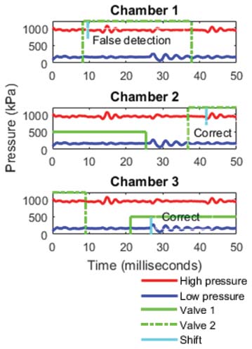
Figure 5 Example with an underestimated threshold.
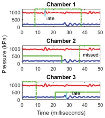
Figure 6 Example with an overestimated threshold.
For an overestimated fixed threshold (i.e., chosen to be very large), the likelihood of missing true shifts increases. Figure 6 shows the shift detection performance with an overestimated threshold. The figure shows that shifts are either detected late or not detected at all.
To overcome the limitations of fixed thresholds, research efforts were proposed to update the decision threshold values in real-time. For example, (Chehade et al., 2017) proposed a real-time failure threshold estimation approach based on the available multisensory signals. (Chang et al., 2011) proposed a dynamic threshold for stock trading signal detection. (Cho et al., 2010) proposed a dynamic decision threshold level for improving upstream transmission performance.
Similarly, rather than using a fixed sensitive threshold, this work proposes a dynamic threshold that depends on the delay time distribution of historical cycles. Specifically, after a valve is opened, an instantaneous change in the pressure reading is expected. However, due to response delays in pump motors, the shift occurs a few milliseconds later. Furthermore, the delay probability distribution can be estimated from historical data and domain knowledge. Consequently, after opening a valve the chances of observing a shift increase with time and it is expected not only after observing a sufficient change in the pressure but also at the time where the delay probability is large enough. Therefore, the proposed dynamic threshold is more appropriate for delay estimation and robust to noise.
Delay Probabilistic Model
The delay in the response time of electric devices is typically stochastic and changes with time. Similar to other stochastic quantities, it is proposed to model the delay as a random variable. In particular, the delay in opening valve v at chamber c is assumed to follow the normal distribution
| (4) |
Where
| (5) |
| (6) |
K is the number of historical cycles, is the observed delay at historical cycle k for valve v at chamber c.
The normal distribution is just one specific distribution. Other distributions can be considered including the empirical distribution that is solely based on the data. Moreover, for every new recorded cycle, the estimates for the mean and the standard deviation are updated via Equations (5) and (6).
Delay Estimation Algorithm
The proposed model for shift detection is mathematically written as
| (7) |
Where the smoothed values for f(tk) and f(tk−1) are
| (8) |
| (9) |
and the dynamic decision threshold is
| (10) |
Here, tvc is the time that valve v at chamber c is requested to open, S is the number of measurements between times tk−1 and tvc, Φ(·) is the cumulative distribution function of a standard normal distribution. In addition, is smoothed by considering S − 1 previous measurements, and is smoothed by considering only one previous measurement to preserve the ripple dynamics.
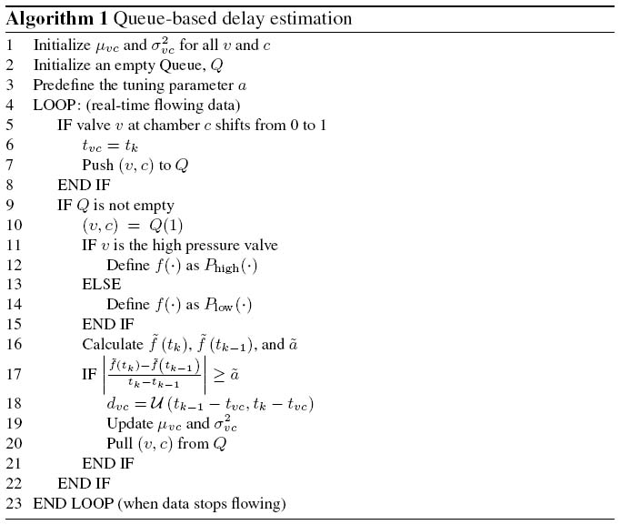
Algorithm 1 describes the proposed delay estimation approach. Initially, the queue is empty and all the valves are closed. The valve (v, c) is pushed into the queue when it shifts from a closed to an opened state. If at least one candidate is in the queue, the algorithm continuously monitors for a shift in the pressure signals. Once a shift is detected, (i) the first valve in the queue is extracted as (v, c), (ii) the delay in opening that valve is estimated by a uniform random number between tk−1 − tvc and tk − tvc to account for the sampling rate of the data acquisition system, (iii) the delay distribution of the valve is updated, and (iv) the candidate (v, c) is pulled out of the queue.
Experimental Setup
Experimental data were collected from a 3-piston in-line digital pump/motor unit, shown in in Figure 7. The unit utilizes two normally closed high speed on/off valves per displacement chamber, one mounted at the high pressure port and the other mounted at the low pressure port, for a total of six valves. The valves implemented on the test stand were Sun Hydraulics DTDA-XCN valves with a 770-212 12V coil.
National Instruments hardware and software was used for data acquisition and control. A four-Slot PXI-1031 chassis was used along with a Field Programmable Gate Array (FPGA) card. A PXI-8108 real time controller, running at 5000 Hz (up to 2.53 GHz), was used to execute a Matlab/Simulink model which contained all the sensor calibration curves. NI Veristand was used to interface between the FPGA and Matlab/Simulink. This allowed the data to be acquired every 0.2 milliseconds.
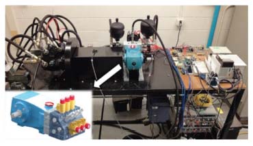
Figure 7 Three piston digital pump/motor test stand (Breidi, 2016).
The pump/motor unit was operated at a pressure of 70 bar, a shaft speed of 700 rpm, and at 100% displacement.
Results
To test the accuracy of the model, actual delay times were experimentally measured using the difference between the time that the signal was sent and the time at which the valve opened. The time when the valve command was sent was recorded, denoted by a black dotted line in Figure 8. The time was recorded for a moment after the signal was sent to account for the 0.2 millisecond data acquisition and to ensure that the signal was fully sent.
The time that the valve opened was recorded using the in-cylinder pressure transducer and was approximated using the moment that the in-cylinder pressure began to spike due to being connected to the high pressure line, shown in Figure 9.
Figure 10 shows the shift detection performance with the dynamic threshold. The figure indicates that the dynamic threshold results in better performance than an overestimated/underestimated fixed threshold. The right peaks were accurately detected over the entire tested cycles.
A comprehensive video for 1000 milliseconds of operation is attached with the supplementary files to help visualize the performance of the detection model. In addition, the next two sections provide more details on the dynamic threshold model and the delay estimation algorithm.
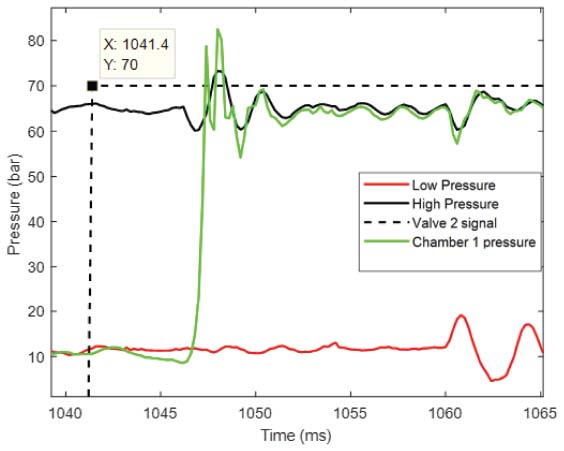
Figure 8 Signal timing.
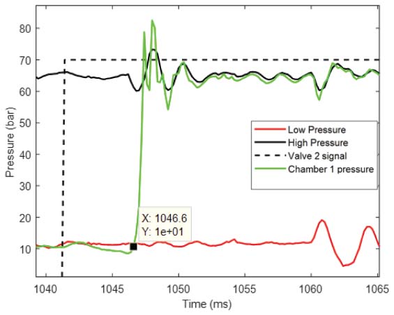
Figure 9 Valve open timing.
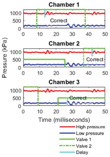
Figure 10 Example of the dynamic threshold model on a digital pump/motor setup.
Table 1 The estimated delays versus the manually calculated delays
| Manually Calculated Delays (Milliseconds) (μvc, σvc) | Estimated Delays (Milliseconds) (μvc, σvc) | |
| (V1, C1) | (5.37, 0.13) | (5.31, 0.057) |
| (V1, C2) | (5.60, 0.14) | (5.71, 0.070) |
| (V1, C3) | (5.39, 0.090) | (5.50, 0.064) |
| (V2, C1) | (5.33, 0.12) | (4.91, 0.062) |
| (V2, C2) | (4.84, 0.10) | (4.90, 0.069) |
| (V2, C3) | (4.47, 0.11) | (4.49, 0.055) |
Table 1 summarizes the experimentally calculated delays and the algorithm estimated delays based on Algorithm 1. Specifically, the mean and standard deviation of the delay for 70 cycles (i.e., around 6000 milliseconds of operation). The experimentally calculated delays are based on manual peak detections in the in-cylinder pressures. The experimentally calculated delays are considered to be close enough to the true delays and serve as the comparison basis for the delays. The table shows that the mean and standard deviation of the estimated delays are very close to that of the manually calculated delays. The table provides clear evidence that the proposed Algorithm 1 accurately and reliably estimates the delay with a 95% confidence interval that is within 2 samples (0.4 milliseconds) of the manually calculated delay.
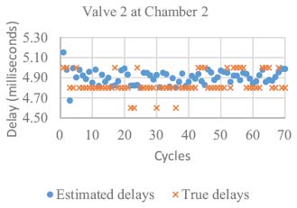
Figure 11 Estimated delays vs true delays for (V2, C2).
For better comparison between the calculated delays and the estimated delays, Figure 11 shows the estimated and calculated delays over the 70 cycles of Valve 2 at Chamber 2. Not only does this show the accuracy of the proposed method in detecting the valve delays in real-time, but it also accounts for the error due to the sampling rate of the data acquisition system of 0.2 milliseconds, which wasn’t considered in the existing approaches, resulting in more realistic estimations for the delays. The figure provides enough confidence in the predictions and performance of the proposed delay estimation algorithm.
Figure 12 further shows the distributions of the predicted delays for the six valves. Every red dot represents the delay estimate of one cycle. The Probability Density Function (PDF) is shown on the left side of the figure and the Cumulative Distribution Function (CDF) is shown on the right side. The figure shows a symmetric and normal spread of the predicted delays around the center of the fitted distributions, which is a major observation that validates the choice of the normal distribution.
Figure 13 shows the sample quantiles of the actual delays versus the quantiles of the estimated distributions shown in Figure 12. While the normality assumption holds only for the range −1 and 1, that range covers the first quartile, the median, and the third quartile. Furthermore, the low standard deviation shown in Figure 15 in comparison to the mean value shown in Figure 14 introduces high sensitivity in fitting a distribution for the delays and also suggests that the mean value by itself is a good estimate regardless of the distribution assumption.
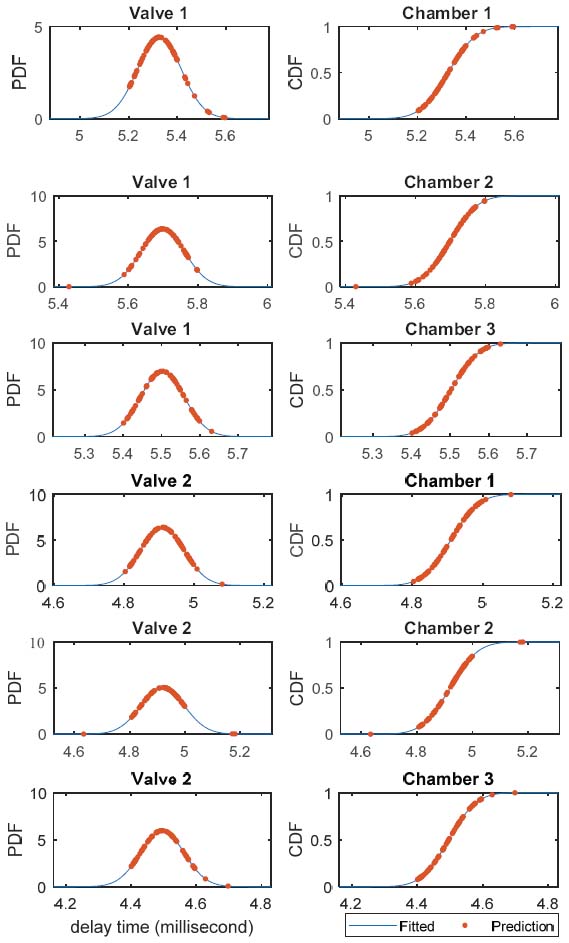
Figure 12 Delay time distributions for the six digital pump/motor on/off valves.
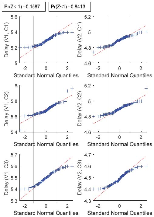
Figure 13 Normal probability plot showing the actual delay quantiles versus the estimated distribution quantiles for the six digital pump/motor on/off valves.
Finally, Figures 14–16 show the adaptive mean, standard deviation, and threshold for the entire 6000 milliseconds, respectively. The initial values for the mean of the delay is chosen based on domain knowledge to be 5 milliseconds, the standard deviation is chosen to be 0.1 milliseconds and the threshold is selected based on another training dataset based on the distance of the highest peak and the mean value in that dataset. As shown in the Figures, the mean, standard deviation, and threshold adaptively change for each of the six digital pump/motor on/off valves. This provides another reason for the high accuracy of the proposed algorithm.
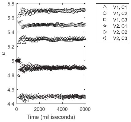
Figure 14 The adaptive mean of the estimated delays.
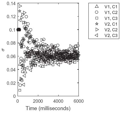
Figure 15 The adaptive standard deviation of the estimated delays.
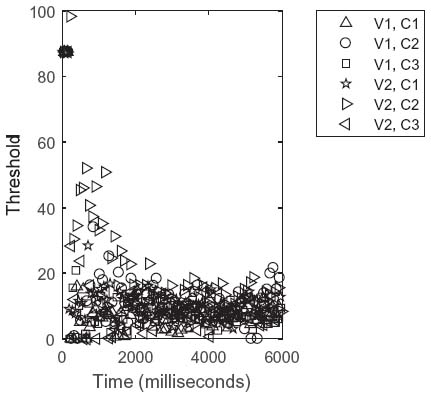
Figure 16 The adaptive threshold as a function of time.
Conclusion
This paper shows the development and evaluation of a statistical based thresholding model which adaptively estimates real-time valve delays that can be used for digital Pump/Motors to improve efficiency in hydraulic systems. The contributions of the paper are multifold: first, an automated statistically data-driven algorithm is proposed to estimate the delay in realtime during operation. Second, a probabilistic model is provided for the delays to quantify the uncertainties and confidence of the estimated delays. To validate the effects of the this model, real time data was acquired and analyzed using pressure transducers to measure and approximate the valve delays for a hydraulic system including an 3 piston in-line pump/motor and 6 on/off solenoid valves. The model was then compared to this real time data to determine the effects of the model. The results prove the algorithm to be successful in measuring and adapting the threshold for real time valve delays.
References
Batdorff, M. A. 2010. “Transient Analysis of Electromagnets with Emphasis on Solid Components, Eddy Currents, and Driving Circuitry”. PhD Dissertation, Purdue University, West Lafayette, In.
Breidi, F., Helmus, T., and Lumkes, J. 2015. The Impact of Peak-And-Hold and Reverse Current Solenoid Driving Strategies on the Dynamic Performance of Commercial Cartridge Valves in a Digital Pump/Motor. International Journal of Fluid Power, http://dx.doi.org/10.1080/14399776.2015.1120138
Breidi, F. 2016. Investigation of Digital Pump/Motor Control Strategies. Ph.D. thesis, Purdue University, West Lafayette, In.
Breidi, F., Garrity, J., and Lumkes, J. 2017. Investigation of a Real-time Pressure Based Valve Timing Correction Algorithm, Proceedings of the ASME/Bath Symposium on Fluid Power and Motion Control, Sarasota, FL., FPMC20174342.
Breidi, F., Garrity, J., and Lumkes, J. 2017. Design and Testing of Novel Hydraulic Pump/Motors to Improve the Efficiency of Agricultural Equipment. American Society of Agricultural and Biological Engineers, Transactions of the ASABE, https://doi.org/10.13031/trans.11557.
Breidi, F., Helmus, T., and Lumkes, J. 2015. “High Efficiency Digital Pump/Motor”, Fluid Power Innovation & Research Conference (FPIRC15)
Chang, P., Liao, W., Lin, J., and Fan, C. 2011. A Dynamic Threshold Decision System for Stock Trading Signal Detection. 11(05):3998–4010. doi:10.1016/j.asoc.2011.02.029.
Chehade, A., Bonk, S., and Liu, K. 2017. Sensory-Based Failure Threshold Estimation. IEEE Transactions on Reliability. 66(03):939–949. doi:10.1109/TR.2017.2695119.
Cho, S., Lee, S., and Shin, D. 2010. Improving Upstream Transmission Performance Using a Receiver with Decision Threshold Level Adjustment in a Loopback WDM-PON. 16(03):129–134. doi:10.1016/j.yofte.2010.01.004.
Holland, M. A. 2012. Design of Digital Pump/Motors and Experimental Validation of Operating Strategies. Ph.D. thesis, Purdue University, West Lafayette, In.
Ivantysyn, J. and Ivantysynova, M. 2003. Hydrostatic pumps and motors. (S. N. Ali, Trans.) New Delhi, India: Tech Books International. (Original work published 1993).
Linjama, M. 2011. Digital Fluid Power-State of the art. The Twelfth Scandinavian International Conference on Fluid Power. Tampere.
Love, L. (August 17, 2009). Fluid power research: A fundamental concern for U.S. energy policy [PowerPoint slides]. Presented at the National Fluid Power Association Industry and Economic Outlook Conference, Wheeling, IL.
Love, L. (March 5, 2014). Energy Impact of Fluid Power [PowerPoint Slides]. Presented at the 2014 IFPE Technical Conference, Las Vegas, NV.
Merrill, K. J., Breidi, F., and Lumkes, J. 2013. Simulation Based Design and Optimization of Digital Pump/Motors. Proceedings of the ASME/BATH 2013 Symposium on Fluid Power & Motion Control, Florida, USA.
Merrill, K. J. 2012. Modeling and Analysis of Active Valve Control of a Digital Pump-Motor. Ph.D. thesis, Purdue University, West Lafayette, In.
Nieling, M., Fronczak, F., and Beachley, N. 2005. Design of a virtually variable displacement pump/motor. Proceedings of the 50th National Conference on Fluid Power, 323–335.
Stelson, K. A. and Li, P. Y. 2013. The Center for Compact and Efficient Fluid Power. ASME. Mechanical Engineering. 135(06):S2–S3. doi:10.1115/ 1.2013-JUN-4.
Biographies

Abdallah A. Chehade received the B.S. degree in Mechanical Engineering from the American University of Beirut, Beirut, Lebanon, in 2011 and the M.S. degree in Mechanical Engineering, the M.S. degree in Industrial Engineering, and the Ph.D. in Industrial Engineering from the University of Wisconsin-Madison in 2014, 2014, and 2017, respectively. Currently, he is an Assistant Professor in the Department of Industrial and Manufacturing Systems Engineering at the University of Michigan-Dearborn. His research interests are data fusion for process modeling and optimization of data-analysis. Dr. Chehade is a member of INFORMS, IEEE, and IISE.

Farid Breidi is an Assistant Professor at the University of Southern Indiana. He received his B.E. in Mechanical Engineering from the American University of Beirut in 2010, M.S. in Mechanical Engineering from the University of Wisconsin-Madison in 2012, and Ph.D. in fluid power from Purdue University in 2016. His research interests include digital fluid power and modeling of dynamic systems.

Keith S. Pate is a Supplier Quality Engineer at Allison Transmission. He received a dual undergraduate degree in General Engineering and Mechanical Engineering from the University of Southern Indiana in 2019. His interests include mechanical design, fluid power, and automotive engineering.

John Lumkes received the B.S.E. degree from Calvin College in 1990, M.S.E. from the University of Michigan-Ann Arbor in 1992, and Ph.D. from the University of Wisconsin-Madison in 1997. From 1997–2004 he was an Assistant and Associate Professor at Milwaukee School of Engineering. In 2004 he joined Purdue University where he is a Professor and is active in digital hydraulics.
International Journal of Fluid Power, Vol. 20_3, 271–294.
doi: 10.13052/ijfp1439-9776.2031
© 2020 River Publishers