Data-Driven Serial Testing of Axial Piston Units: Integrating Signal Processing and Machine Learning for Roller Bearing Fault Detection
Maximilian Romeser1, 2,* and Reinhold von Schwerin1
1Faculty for Informatics, Ulm Technical University of Applied Sciences, Ulm, Germany
2Development of Axial Piston Units, Bosch Rexroth AG, Elchingen, Germany
E-mail: maximilian.romeser@boschrexroth.de; reinhold.vonschwerin@thu.de
*Corresponding Author
Received 31 August 2025; Accepted 26 January 2026
Abstract
Data-driven fault detection is crucial for hydrostatic drives and axial piston units (APUs) due to their central role in both conventional and electrified powertrains. The reliability of their internal roller bearings is pivotal to prevent machine downtime and guarantee high efficiency. However, detecting bearing faults in End-of-Line (EoL) serial testing for quality control is particularly challenging. Strong hydraulically induced noise and, most notably, significant manufacturing-related serial dispersion across units often mask the subtle fault signatures. To address this, this paper introduces a novel experimental methodology designed to simulate a realistic EoL scenario. By systematically interchanging drive shafts and housings among a set of seven units to create 30 unique component combinations, the inherent serial dispersion found in production is effectively replicated. This innovative approach allows for the efficient testing of distinct manipulted bearings against a realistic backdrop of component variability. Using vibroacoustic data from this setup, the present study integrates semi-supervised machine learning (ML) with a comparative analysis of different sensors and signal processing techniques. It is demonstrated that a fixed accelerometer on the test bench, when combined with a knowledge-based bandpass filter for envelope spectrum analysis, provides the most robust fault detection. This optimized configuration consistently achieves an Area Under the Curve (AUC) exceeding 0.95, effectively separating faulty from healthy units despite the challenging conditions. The findings provide a clear framework for implementing a reliable and automated fault detection system in industrial manufacturing, proving that data-driven quality control can succeed even in high-variance, noisy production environments.
Keywords: Axial piston units, fault detection, anomaly detection, vibroacoustic analysis, machine learning, condition monitoring, serial testing, roller bearings.
1 Introduction
The robustness and high power density of hydrostatic drivetrains have long established them as a preferred choice in off-road applications. These systems are particularly valued for their precise control accuracy, high dynamics, and the ability to provide stepless transmission. Additionally, hydrostatic drives enable linear movements for various work functions, making them indispensable in demanding environments [1]. Given these advantages, hydrostatic drives, and APUs in particular, play a central role in the powertrain, whether it is a conventional drivetrain with an internal combustion engine or an electrified drivetrain, as shown in [2]. Therefore, the reliability of APUs is vital to prevent costly maintenance and machine downtime. As a result, methods for fault detection and diagnosis are the focus of various research efforts, primarily to enable condition monitoring (CM) and predictive maintenance, which are already well-established for gearboxes and turbines [3]. Additionally, robust and automated fault detection can serve as a valuable quality control measure during serial testing, particularly when products are in the ramp-up phase of production. Monitoring changes in suppliers is also crucial in this context.
Regarding the reliability of rotating machinery in general, and especially APUs [4], roller bearings are essential components [5]. Consequently, the detection of faulty bearings constitutes a significant area of research. In this context, the analysis of vibroacoustic behavior has emerged as an effective tool, enabling the detection of fault-related geometric deviations through anomalous excitations during operation [5]. This allows the detection of most failures in rotating machinery at an earlier stage than by monitoring temperatures or other signals [3] [6]. However, in the case of axial piston units (APUs), this is particularly challenging compared to other rotating machinery. The abrupt impulses induced by the reciprocating pistons are extremely dominant, making it difficult to detect fault-induced anomalies in the emitted structure-borne or airborne noise (SBN or ABN) [4]. Furthermore, when considering scenarios for fleet-based CM [7] or serial testing processes, it is important to account for serial dispersion. Conventional CM approaches typically assume a nominal reference state for the machine under consideration, where the signal behavior is initially stable, and faults manifest as anomalies relative to this reference. However, in the aforementioned scenarios, such an approach is not feasible due to the short testing duration, varying operating conditions and the potential presence of initial faults. Instead, anomalies in the data of new test units must be evaluated in relation to the historical data of previous, healthy units. Due to serial dispersion, the vibroacoustic behavior also varies, and fault-induced anomalies must be sufficiently pronounced to stand out against this variability [8].
Given the complexity of the vibroacoustic and structural dynamic behavior of APUs, this study aims to develop a data-driven approach based on measurements from an ensemble of units. The approach follows the concept of semi-supervised anomaly detection and falls within the field of ML and AI. An ensemble of tested, healthy units will be used to characterize production variability and train the model, while various faulty units will be evaluated during model testing. Since it is not straightforward to determine how fault patterns manifest in vibroacoustic behavior and emissions, different signal processing and feature generation methods will be investigated. The goal is to extract fault-relevant information from the data to ensure robust, data-based fault detection. Since vibroacoustic behavior can be highly dependent on operating conditions and sensor application, these factors will be comprehensively evaluated to provide a holistic assessment of fault detection and to determine the optimal conditions for serial testing processes. To the best of the author’s knowledge, no study has yet explored the data-driven detection of faulty roller bearings in an ensemble of APUs. Therefore, the contributions of this study are as follows:
• Proposal and evaluation of a semi-supervised approach for detecting APUs with faulty roller bearings in an experimental serial testing scenario using ML
• Evaluation of the combination of various approaches for signal processing and feature generation under various operation conditions
• Comparison of different sensor applications for analysis of vibroacoustic behavior of APUs
To provide an overview of the study’s scope, all varied conditions and methods within the proposed pipeline are illustrated in Figure 1.
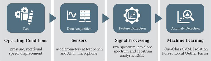
Figure 1 Varied conditions and methodological components of the study.
2 Related Work
Fault diagnosis of APUs – including fault detection as well as fault identification – has become a prominent field of research in recent years, driven by advancements in ML and signal processing, as shown in [9]. Typically, this research is conducted within the framework of CM or in a more general context. Only Gaugel et al. [10] consider a serial testing scenario of APUs, without delving into the specific faults and signals and instead focusing on time series segmentation. In the following, the authors of this paper limit themselves to studies regarding fault diagnostics of APUs utilizing vibroacoustic analysis. In particular, data-driven approaches including advanced signal processing and ML techniques are frequently discussed in this context, as physical model-based approaches are very challenging due to the system’s complex and nonlinear vibroacoustic behavior [11]. Within the scope of ML-based fault diagnosis, two primary learning paradigms can be employed:
• Supervised learning for classification and regression tasks relies on extensive datasets where all fault types are clearly labeled. Thus, it is not only suitable for fault detection but for both fault isolation and fault identification as well.
• Semi-supervised learning for anomaly detection is relevant for fault detection, especially when labeled fault data is scarce or when novel, unknown fault patterns need to be identified. This approach primarily models the normal operating state, flagging any significant deviation as an anomaly, thus focusing on detection rather than specific fault identification.
A comprehensive study on the use of conventional ML approaches in terms of supervised classification for CM scenarios is provided by Torrika [12], who particularly highlights the steps of feature extraction and reduction. An analogous approach to feature generation in a supervised classification setting can be found in [13]. Further intensive research on the condition monitoring (CM) of axial piston pumps using supervised methods such as Support Vector Machines (SVMs) and gradient boosting algorithms, utilizing a feature engineering approach based on tsfresh [16], was conducted by Horn et al. [14, 15]. In contrast, Gnepper et al. [17] and Siyuan et al. [18] explore a semi-supervised anomaly detection scenario and employ principal component analysis (PCA) to characterize the nominal state of the APU within the context of CM.
To better highlight fault information, signal processing techniques such as Fast Fourier Transformation (FFT) [17, 19, 20], Wavelet Packet Transformation (WPT) [9, 18, 19], Empirical Mode Decomposition (EMD) [20], Cepstrum Analysis [11], or Time Synchronous Averaging [13] are frequently employed. Specifically, in the detection of faulty bearings in APUs, various techniques are commonly employed to generate sensitive filter bands and enhanced signal envelopes [4, 19–22]. For the fault detection of worn slippers, the principle of cyclostationarity plays a particularly important role here, as investigated by Casoli et al. [25]. By considering the results in [19], it can be observed that commonly studied fault patterns, such as wear on slippers, port plates or cylinders, can have immediate effects on the dominant harmonics of the piston frequency. However, this is not the case for roller bearings, which imposes different requirements on signal processing. Advanced signal processing techniques also support the application of Deep Learning (DL) utilizing deep artificial neural networks (ANNs), which has been extensively studied in the context of fault detection for APUs in recent years [24–31]. As such, model training typically involves feature extraction based on scalograms (based on Continous Wavelet Transformation or CWT) or spectrograms (based on Short Time Fourier Transformation or STFT), rather than directly utilizing the raw time series data as in [33]. However, being supervised classification settings the foundation of these approaches relies on the identification of known, specific fault states resulting from wear and damages, as well as on sufficient data volumes without considering serial dispersion due to manufacturing tolerances. As Keller et al. [34] emphasize, this must be ensured for adequate validation. Nevertheless, in the case of CM, these factors are frequently irrelevant, since the goal is to identify faults relative to the normal condition of the same unit, as mentioned before. This contrasts with the present use-case.
Although the developed methods are often tested at various operating conditions, only Horn et al. [14, 15] and Gnepper et al. [17] investigate a wide operating range and determine the quality of fault detection with respect to slipper clearance or also slipper wear and valve plate cavitation [14] depending on this range. Additionally, while the experimental setups of some of the mentioned studies include multiple SBN or ABN sensors, such as in [4] or [9], this aspect is not always analyzed in detail. Casoli et al. [13, 19, 25] and Du et al. [11], for instance, only consider SBN in axial and radial directions, whereas Gnepper et al. [17] analyze different sensor concepts and positions. Furthermore, the investigations in [34] indicate that positioning the sensor close to the bearing is effective, even when the valve plate is damaged. Other studies address the fusion of multi-sensor data and transfer learning, including acoustic signals [33] or pressure signals [26].
Upon closer examination of the cited works, their data-driven pipelines can be grouped into four categories (see Figure 2) based on the utilization of ML or DL and upstream signal processing techniques:
1. Direct feature-based ML
2. Signal processing-based ML
3. Hybrid DL
4. End-to-end DL
While purely physics-based models can function independently of any data, all of the aforementioned approaches require datasets due to their data-driven components. Notably, the integration of domain knowledge through advanced signal processing steps is often more convenient than fully end-to-end DL approaches. This highlights a practical trade-off between the level of expert input required and the volume of training data available. It is also important to note that, in the context of conventional ML, a strict separation between signal processing and feature extraction is not always feasible. For instance, coefficients obtained from a signal processing technique such as WPT [9] can serve directly as features for an ML model, altough a step of feature selection can be integrated which is neglected in Figure 2. Conversely, in DL pipelines, a clearer distinction can be made between hybrid and end-to-end approaches. Nevertheless, actual feature extraction is handled inherently by the neural network in both cases. Table 8 in the appendix maps the works including complete data-driven pipelines to this taxonomy and the two learning paradigms discussed earlier, while also adressing the sensors used, the range of operating conditions studied, and the considered faulty components. Hence, related work only covering signal processing is not considered. It is obvious, that most of the mentioned works are related to supervised scenarios with known fault states without considering bearing faults.
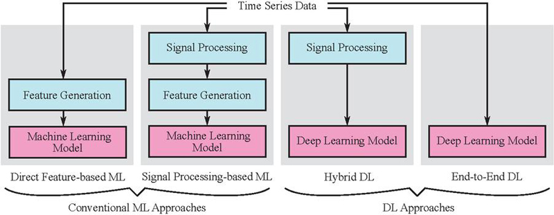
Figure 2 Categorization of ML and DL approaches regarding vibroacoustic fault detection in APUs referring to the complete pipelines: Data-driven (trainable) components are highlighted in pink, while predefined (fixed) components are shaded in cyan.
Table 1 Overview of methods and models in reviewed works (CWT: Continuous Wavelet Transformation, CNN: Convolutional Neural Network, kNN: k-nearest-neighbor, DT: Decision Tree, MED: Medium Entropy Deconvolution, FFT: Fast Fourier Transform, STFT: Short-Time Fourier Transform, WPT: Wavelet Packet Transform, EMD: Empirical Mode Decomposition, TSA: Time Synchronous Averaging)
| Work | Category | Signal Processing | Learning Paradigm | Model |
| [27] | 3 | CWT | Supervised | CNN |
| [33] | 4 | – | Supervised | CNN |
| [34] | 2 | FFT | Supervised | kNN, DT |
| [26] | 3 | STFT | Supervised | CNN |
| [28] | 3 | CWT | Supervised | CNN |
| [29] | 3 | CWT | Supervised | CNN |
| [30] | 3 | CWT | Supervised | CNN |
| [9] | 2 | WPT | Supervised | ANN |
| [31] | 3 | MED | Supervised | CNN |
| [19] | 2 | FFT | Supervised | Multiple |
| [32] | 3 | CWT | Supervised | CNN |
| [20] | 1, 2 | FFT, WPT, EMD | Supervised | SVM |
| [17] | 2 | FFT | Semi-supervised | PCA |
| [18] | 2 | WPT | Semi-supervised | PCA |
| [13] | 1, 2 | TSA, FFT | Supervised | Multiple |
| [12] | 1, 2 | FFT, CWT | Supervised | Multiple |
| [14] | 1 | – | Supervised | SVM, XGBoost |
Table 2 Overview of operating conditions and faulty components in reviewed works (SBN: Structure-Borne Noise, ABN: Air-Borne Noise)
| Work | Signal | Operating conditions | Faulty components |
| [27] | ABN | Single | Swash plate, slipper, center spring |
| [33] | SBN, ABN | Few | Slipper, piston, valve plate |
| [34] | SBN | Few | Valve plate |
| [26] | SBN, pressure | Single | Slipper |
| [28] | SBN, ABN, pressure | Single | Swash plate, slipper, center spring |
| [29] | SBN | Single | Swash plate, slipper, center spring |
| [30] | SBN | Single | Swash plate, slipper, center spring |
| [9] | SBN | Single | Valve plate |
| [31] | SBN | Single | Piston, cylinder, shaft |
| [19] | SBN | Few | Port plate, slipper, cylinder |
| [32] | ABN | Single | Swash plate, slipper, center spring |
| [20] | SBN | Single | Piston |
| [17] | SBN | Multiple | Slipper |
| [18] | SBN | Single | General |
| [13] | SBN | Few | Port plate, slipper, cylinder |
| [12] | SBN | Few | Slipper, Roller bearing, cylinder |
| [14] | SBN, pressure | Multiple | Slipper, valve plate |
3 Experimental Design
Given the lack of publicly available datasets and prior work on fault detection in APUs, an experimental campaign is necessary to realize the proposed serial testing scenario. To facilitate testing of a sufficient number of both healthy and faulty units, the campaign is conducted on a laboratory test bench using an ensemble of such units. The experimental design, including the materials and the test sequence, as well as the data acquisition setup is described below.
3.1 Material and Fault Types
In this study, an ensemble of seven APUs in bent axis design were tested using a laboratory hydraulic test bench, as shown in Figure 3. The hydraulic scheme of the test bench is shown in Figure 4. Each APU was initially tested in its original delivery condition. Subsequently, to characterize the range of vibroacoustic variation attributable to component interchangeability, the drive shafts were systematically interchanged among the housings. For example, in the first round of swaps, the drive shaft from the first APU was placed into the second housing, the second unit’s drive shaft into the third housing, and so on. While a full exploration of all 49 possible unique pairwise combinations was desirable, time constraints limited this cross-assembly testing, constituting the first phase of the experimental series, to 30 unique drive shaft-housing combinations (achieved through 23 swaps). Throughout this phase, the rotary groups remained equipped with their original, undamaged bearings, which were not removed. This approach enabled assessment of vibroacoustic variability while isolating the effects of drive shaft and housing variations.
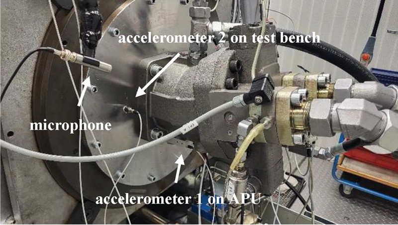
Figure 3 Experimental setup at the laboratory test bench.
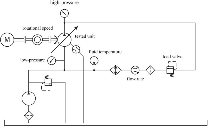
Figure 4 Simplified hydraulic scheme of the setup used at the laboratory test bench.
In the second phase of the experimental series, 14 rotary groups with faulty roller bearings are installed. The rotary group essentially consists of the drive shaft, the pistons, the cylinder, as well as a large and a small cylindrical roller bearing that support the drive shaft within the housing. In 12 cases, the fault concerns the large roller bearing, and in two cases, the small roller bearing. Faults in other components of the rotary group are neglected for the purposes of this investigation, meaning that these components remain in a healthy condition. The types of faults in the tapered roller bearings are intentionally chosen to be heterogeneous to generate a broad portfolio of potential anomalies in the data and to ensure comprehensive validity. The bearings are manipulated, with different sections of the raceways or end faces of the rolling elements abrasively processed, as exemplarily depicted in Figure 5. The defects vary in depth and width, as well as in number and location of the defects (see Table 9 in the appendix). Regarding further investigation, it is crucial to generate both easily detectable faults (e.g., signals with significantly higher signal energy) and subtle faults, identifiable only by the presence of small peaks in the frequency spectrum, to evaluate the robustness of the fault detection method. Due to modulation effects resulting from tolerances in the APU, various effects of impact excitations on the SBN emissions are observed. It should be noted that due to the cage, subsequent processing of the inner ring is not possible. Each faulty rotary group is mounted once in one of the housings, and the assembled unit is then tested on the test bench. The assignment of faulty rotary groups to housings is done randomly.
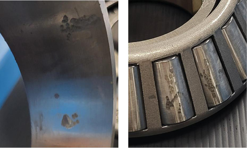
Figure 5 Examples for faulty roller bearings within the experimental test campaign. Left: Outer ring raceway. Right: Rolling elements.
3.2 Test Sequence
Each unit or rotary group-housing combination, regardless of the presence of a fault, undergoes the same automated test sequence on the test bench for high reproducibility. Initially, a run-in period with a duration of 15 min is conducted to achieve an fluid temperature level of 40∘C. Since the regulation is not perfect, fluctuations can occur during operation, especially when load points are varied. In the end, the overall fluid temperature range, across all following load points, was 42∘C to 56∘C. For individual load points, the experimentally determined temperature variation did not exceed 8∘C, as depicted in Figure 6. It is plausible that these fluctuations, particularly in relation to fluid viscosity, may influence the vibroacoustic emissions. However, varying fluid temperatures can also occur in real serial testing, and thus, it is treated as regular process variation. In general, the fluid temperature correlates with the high-pressure, as the mechanical energy of the electric motor is converted into heat due to the load valve in the hydraulic circuit (see Figure 4).
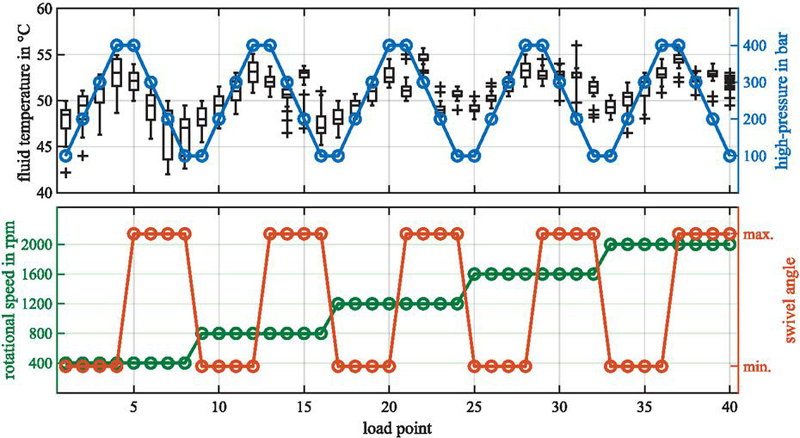
Figure 6 Variation in fluid temperature across different load points with boxplots summarizing the tests performed.
The test procedure involves the traversal of a three-dimensional operating range with the three factors influencing the current load point. A load point is defined by the shaft speed, the pressure in the high-pressure line, and the swivel angle or displacement, respectively. The load in the closed circuit is adjusted in four stages between 100 and 400 bar using the variable load valve. The speed is varied in five equally sized stages between 400 and 2000 rpm. The swivel angle is set to either its minimum or maximum position. The swivel angle as well as the high-pressure influence the bearing load (BL), which is why these parameters are referenced accordingly in Table 3 for clarity. For example, higher pressures increase the axial load on the bearings, while the swivel angle alters the internal force distribution within the drive mechanism. This affects rolling behavior and may influence both noise emission and hydraulic pulsations. Consequently, the resulting section of the test sequence includes 40 load points (see Figure 6). Between the load points, the operating conditions are adjusted in a ramp-like manner. Each load point is then held for 10 s.
Table 3 Indexing of the different bearing loads (BLs)
| BL | 1 | 2 | 3 | 4 | 5 | 6 | 7 | 8 |
| Pressure [bar] | 100 | 200 | 300 | 400 | 400 | 300 | 200 | 100 |
| Swivel angle | Min. | Min. | Min. | Min. | Max. | Max. | Max. | Max. |
3.3 Sensors and Data Acquisition
To capture the vibroacoustic behavior, three sensors were applied: Firstly, a free-field microphone is permanently installed to measure ABN, as shown in Figure 7, at approximately 30 cm above the APU. Secondly, a triaxial piezo-electric accelerometer is permanently attached to the test bench using an adhesive adapter to capture SBN emissions (accelerometer 2). Since the sensor application is performed just once before the test series, high reproducibility of the results is ensured. This permanent application is particularly advantageous for serial testing, as it eliminates the need for manual sensor placement by the operator or automatic positioning systems. Additionally, it is beneficial to measure as close as possible to the relevant source of SBN, i.e., the roller bearing, to achieve a high signal-to-noise ratio (SNR). For this purpose, another accelerometer of the same type is permanently mounted using an anodized screw adapter, as shown in Figure 7 (accelerometer 1). The adapter is attached to the bolting of the bearing cross-flushing and is therefore reattached with each new unit mounted on the test bench, i.e., for each test. Consequently, this has a negative impact on the dispersion between the conducted tests.
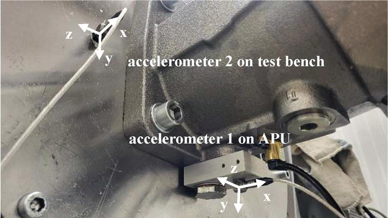
Figure 7 Detailed view of the attached accelerometers.
The sampling rate is consistently set to 50 kHz. To avoid aliasing effects, a Butterworth low-pass filter with a cutoff frequency of 25 kHz is employed. Data acquisition is performed in intervals and controlled by an automated test sequence. After a stabilization period of three seconds, interval measurements of 5 s duration are conducted at each of the 40 load points. For further investigations, the signals or time series from the different vibroacoustic sensors are referenced as shown in Table 4. Consequently, the relevant dataset consists of 40 x 7 x 44 time series with each time series comprising 250000 samples. Consequently, there are 40 x 7 data subsets including 44 time series per each.
Table 4 Notation of the different signals from each sensor used for capturing the vibroacoustic emissions of the tested units
| Sensor | Microphone | Accelerometer 1 | Accelerometer 1 |
| Signal names | Lp | a1x, a1y, a1z | a2x, a2y, a2z |
| Captured emission | ABN | SBN | SBN |
| Unit |
4 Data-Driven Methodology
The methodology employed in this paper to generate a data-driven fault detection model is based on a modular, semi-supervised framework comprising three stages: signal processing, feature generation, and anomaly detection. The first two stages are collectively referred to as feature extraction (see Figure 1), while the final stage encompasses the actual ML. The entire framework, shown in Figure 8 enables seamless substitution of methods at each step which allows the systematic evaluation of multiple signal processing techniques and anomaly detection models across the signals of different sensors and load points. First, signal processing methods including various approaches for envelope spectrum (ES) analysis can be used to pre-emphasize fault‑related characteristics in the signal without training. Next, features are generated depending on the domain and serve as the input for the semi-supervised anomaly detector. Finally, the latter learns the characteristics of normal operation from healthy data and flags anomalies as potential faults using ML.
Importantly, signals from different sensors or load conditions are not merged into a single feature set, as this would create an excessive feature‑to‑instance ratio. Thus, with fewer than 44 instances available for the training of one model after testset separation, DL approaches would risk overfitting and sacrifice interpretability. With reference to Figure 2, therefore, the focus is set on conventional ML approaches that remain robust on smaller datasets. Although real serial testing scenarios can yield large amounts of healthy data overall, the diversity of product variants and operating conditions in the scope of mobile machinery means healthy samples for each configuration are inherently limited. In addition, it is worth noting that conventional ML approaches can outperform DL models when appropriate signal processing techniques and domain knowledge are applied. This has been demonstrated, for example, by Bienefeld et al. [35] using the CWRU dataset [36]. Finally, to evaluate the influence of sensor configuration and loading conditions, as well as the suitability of various signal processing and ML techniques, meaningful performance metrics to enable a robust and comparable assessment are employed.
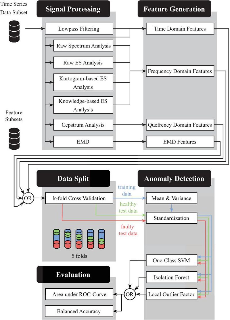
Figure 8 Framework-based integration of the data-driven methodology. The pipeline enables the variation of signal processing techniques and their corresponding features as well as the variation of the anomaly detection model (OR gates). Note that the pipeline is set up for each individual time series data subset regarding different load points and sensor signals. Furthermore, the resulting feature datasets are not mixed considering one model.
4.1 Signal Processing
In the scope of this work, multiple signal processing methods are investigated, each providing a different domain of signal representation. These include:
• Frequency domain (FD) methods, such as raw spectrum analysis and ES analysis, which reveal how signal energy is distributed across different frequency components. This domain is particularly useful for identifying dominant frequencies and harmonic structures related to mechanical behavior.
• Quefrency domain (QD) analysis, based on the cepstrum, which allows the detection of periodic patterns in the frequency spectrum, offering an additional perspective on modulated or repetitive signal content.
• Time domain (TD) approaches, including both direct analysis of the raw time signal and empirical mode decomposition (EMD), which enable the examination of temporal signal characteristics and local variations over time.
These complementary domains offer different insights into the vibroacoustic behavior of APUs, supporting a comprehensive analysis framework. Multiple variants of ES analysis are also explored to assess their suitability for different signal characteristics (see Figure 8). A more detailed overview of the applied methods can be found in Randall et al. [5].
To reduce the influence of high-frequency noise in combination with system-induced resonances, a low-pass filter with a cutoff frequency of 3 kHz was applied prior to signal processing. This choice was guided by visual inspection of the raw time series data and preliminary spectral analysis. Above 3 kHz, the spectra were dominated by broadband excitations strongly influenced by test bench and sensor coupling resonances – most notably in signals from accelerometer 1. These non-deterministic effects varied strongly across individual units and could obscure the APU-specific features of interest. In contrast, the frequency range below 3 kHz consistently captured the most relevant and deterministic information without causing too much dispersion across different units, as illustrated in Figure 9.
Although the measured data are univariate time series instances of the form , where denotes discrete time steps, is the sampling frequency, and is the sequence length, they inherently form sequences of discrete values that can also be represented as vectors . For simplicity, however, they are hereafter partially treated as continuous-time signals .
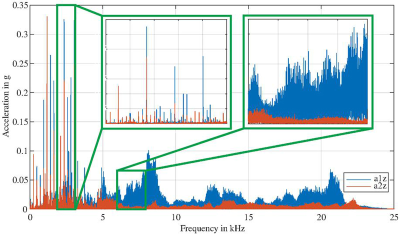
Figure 9 Frequency spectra of a healthy unit considering the z-direction of the accelerometers before low-pass filtering. The section between 2 and 3 kHz predominantly contains deterministic frequency components associated with pump operation, whereas the example section between 6 and 8 kHz exhibits strongly noise-like, non-deterministic characteristics that are heavily influenced by resonances.
4.1.1 Raw spectrum analysis
Bearing faults cause vibrations at characteristic frequencies depending on fault type, operating conditions, and bearing geometry. To interpret and identify these, the discrete signal is transformed into FD using FFT:
| (1) |
where refers one frequency bin. In analogy to the time series, represents a discrete representation of the spectrum in continous FD .
To reduce spectral leakage, which arises when the signal is not perfectly periodic within the analysis window, a hamming window function is applied to the TD signal, i.e., , before performing the actual FFT. This windowing ensures that discontinuities at the edges of the sampled segment are smoothed out, thereby improving the accuracy of the spectral representation, especially for closely spaced fault frequencies. As a consequence, the features become more robust and less sensitive to stochastic variations across different time series. In other words, the overall feature variance within the ensemble of healthy instances is reduced, which enables more reliable anomaly detection with respect to fault-related frequency components.
4.1.2 Envelope spectrum analysis
As the raw signal spectrum often provides limited diagnostic information about bearing faults, ES analysis has become an established method for bearing diagnostics [5]. The envelope-based method exploits the fact that a high-frequency carrier signal, which reflects the structural resonances and is influenced by other excitations, is amplitude modulated by the recurring impulses caused by bearing faults. The relevant information in the raw signal can thus be identified through demodulation, where the envelope can be generated using the Hilbert transform as follows:
| (2) |
and the FFT of this envelope reveals the ES , where again a Hamming window is applied to minimize spectral leakage. It should be noted, however, that the envelope can be significantly affected by piston frequencies, as demonstrated by Xiao et al. [4]. As mentioned by Randall et al. [5], it thus makes sense to identify frequency bands that are primarily dominated by bearing resonances before demodulation.
On one hand, the definition of the filter band can be conducted by using empirical or domain knowledge. In the context of this work, these were determined empirically, and a bandpass filter with a passband of 2 to 3 kHz was chosen for this knowledge-based ES analysis. The lower frequency range (0–2 kHz) was intentionally excluded because it is heavily dominated by the fundamental piston frequencies and their strong harmonics, as well as other process-related hydraulic noise. These powerful, but fault-irrelevant, signals can mask the subtler, high-frequency signatures of bearing faults. The 2–3 kHz band, in contrast, was empirically found to offer a better SNR, where bearing fault resonances are more pronounced relative to the attenuated hydraulic pulsations. This contrasts to the raw ES analysis, which examines the entire frequency band up to 3 kHz without using empirical knowledge.
On the other hand, the identification of a suitable filter is generally non-trivial. However, spectral kurtosis provides a tool that relates the impulsiveness of the signal to its frequency components. The underlying hypothesis is that frequency bands containing information relevant to bearing fault detection exhibit higher spectral kurtosis. For simplicity, a detailed explanation of the method is omitted here, and instead, explicit reference is made to [5]. However, it is important to understand that a window is slid over the time series and an FFT is performed for each window, resulting in the STFT and the spectrogram . This process transforms the signal into the time-frequency domain. The spectral kurtosis is calculated as
| (3) |
with characterizing the time-averaging operator. Frequency ranges with high spectral kurtosis are then suitable filter bands. Determining these ranges depends on the ratio of the window length to the unknown spacing between the periodically occurring impulses. Therefore, the kurtogram is constructed, which further represents as a function of the window length. Due to the time-frequency uncertainty principle, the frequency resolution increases with longer window lengths. The scheme of the kurtogram-based ES analysis is compared with the knowledge-based ES analysis, raw ES analysis and raw spectrum analysis in Figure 10.
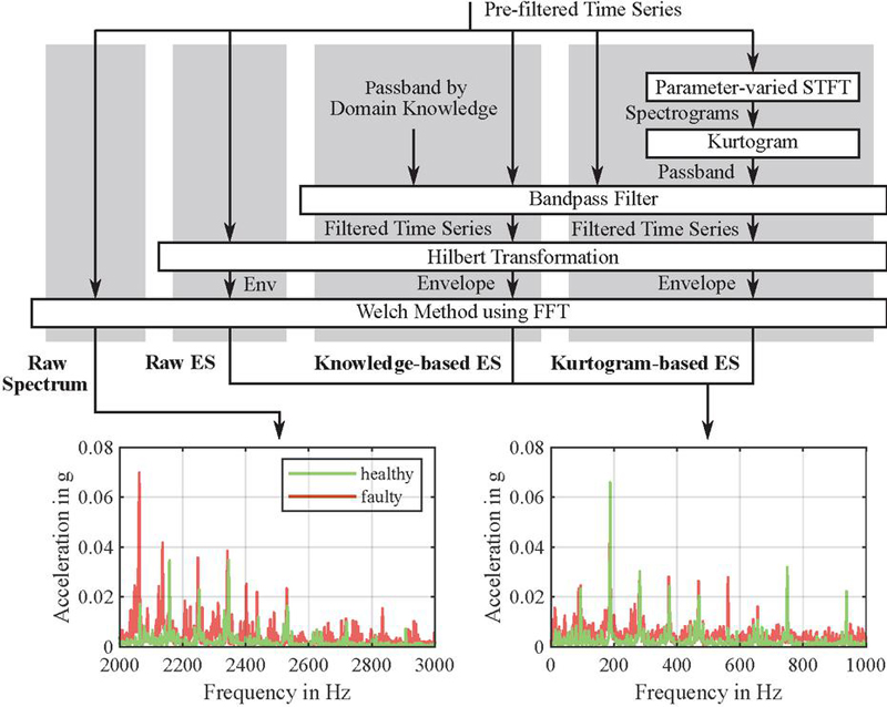
Figure 10 Comparison of the procedures used in the four different spectrum analysis techniques applied in this study. Note that the most relevant parts of the raw spectrum and the ES differ, since the latter highlight information related to the modulation frequency. The depicted ES is based on the knowledge-based ES analysis, whereas the other two ES may differ.
4.1.3 Cepstrum analysis
Another method to reduce the influence of disturbances in relation to fault-induced anomalies is cepstrum analysis. In the cepstrum, families of periodically spaced spectral components appear as prominent peaks, known as rahmonics, which include both harmonics and sidebands in the spectrum. These phenomena are caused by impulsive forces due to roller element bearing faults combined with amplitude modulations resulting from phase shifts between the load and the fault positions [37]. According to Du et al. [11], this approach has been successfully applied in the context of bearing fault detection in APUs.
The cepstrum is generated by first transforming the signal into FD using the FFT. After logarithmizing the spectral amplitudes, the signal is then transformed into QD with , which can be expressed as
| (4) |
In simple terms, the cepstrum represents the inverse transformation of the logarithmized power spectrum , thereby presenting the cepstrum in relation to the quefrency components in TD once again. Hence, the reciprocal quefrency provides insights into dominant families of frequency components.
4.1.4 Empirical mode decomposition
A purely heuristic approach to signal processing is EMD, which enables the decomposition of into so-called Intrinsic Mode Functions (IMFs) and a residual :
| (5) |
The IMFs characterize different frequency bands, which is particularly advantageous for diagnosing faulty roller bearings when there is no prior knowledge of relevant bands or the signal structure. To determine the individual IMFs, the algorithm iteratively decomposes in TD through a process called sifting, which proceeds as follows:
1. Determine the local minima and maxima of .
2. Generate the lower and upper envelope and using the local extrema.
3. Compute the mean of the envelopes: .
4. Subtract from to obtain the residual .
This process is repeated times with until a specific condition is met: In this study, the process is completed after repetitions, resulting in four IMFs and the final residual .
4.2 Feature Generation
Given the diverse nature of fault cases, it is challenging to generate fault-related features in advance, as these may not be suitable for extracting the underlying anomalies from the signal in every fault scenario. It is worth mentioning that, even for roller bearings alone, a multitude of fault cases is possible, which cannot all be considered within the scope of this study. Therefore, it is even more important to develop appropriate features that chararacterize the processed signals in feature spaces where references the feature sets used for the domain. Note that a feature set denotes the predefined set of mathematical operations applied to the (processed) signal, not the feature values themselves regarding one data instance. If the features are to be derived directly from the time series , resulting in a feature vector refering to the -th data instance, statistical metrics are used for this purpose. This includes the first four statistical moments: mean , variance , skewness, and kurtosis, with the latter two defined as
| (6) |
Depending on the amplitude, outliers receive a higher weight. Additionally, the Root-Mean-Square (RMS) and the median are used as features and . Analogous to [34], it makes sense to relate features in FD to specific frequency bands and span . This approach allows, for example, the isolation of bands where bearing faults excite the corresponding bearing resonances [38] from bands where piston frequencies are dominant. Therefore, the spectrum is divided into five frequency bands according to Table 5, and the mean and kurtosis are calculated for each band. The same approach for feature generation can also be applied to the cepstrum in QD by calculating reciprocal values for . In the case of the kurtogram-based ES analysis, it is also useful to use the boundaries of the selected frequency band as an additional feature. Since EMD is performed in TD, the RMS is calculated instead of the mean to characterize signal power and a seperate feature set is needed to span referring to the single IMFs. An overview of the features is given in Table 6. Consequently, the entire time series dataset is divided into 40 x 7 x 7 feature datasets meaning 7 feature datasets are related to one time series data subset depending on different signal channels and load points.
Table 5 Frequency bands for feature generation in FD. The corresponding quefrency bands have reciprocal start and end values
| Frequency band | 1 | 2 | 3 | 4 | 5 |
| Start frequency [Hz] | 0 | 120 | 360 | 840 | 1800 |
| End frequency [Hz] | 120 | 360 | 840 | 1800 | 3200 |
Table 6 Overview of domain-specific feature sets. Although EMD is also conducted in TD, a seperate feature set is used
| Domain | Set Size | Description of Features |
| Time | 6 | Mean, variance, skewness, kurtosis, RMS, median |
| Frequency | 10 (+ 2) | Mean and kurtosis per band (+ kurtogram-based |
| passband frequencies) | ||
| Quefrency | 10 | Mean and kurtosis per band |
| EMD | 10 | RMS and kurtosis per IMF or residuum |
4.3 ML-based Anomaly Detection
In this study, it is assumed that faulty units generate anomalous data. Given that anomalous data are typically rare, it is often practical for anomaly detection to use normal data to construct a model that can reflect the characteristics of normal data (semi-supervised anomaly detection or novelty detection). These models are then capable of identifying anomalous data based on their deviating characteristics and thus a higher anomaly score. In this study, three ML techniques are employed for anomaly detection (see Figure 8): the One-Class Support Vector Machine (OC-SVM), the Isolation Forest (IF), and the Local Outlier Factor (LOF). The reason for using multiple techniques lies in the fact that it is not trivial to determine which method will yield the best results for a given dataset. By applying these diverse approaches, the goal is to comprehensively evaluate their performance and robustness in detecting anomalies.
To ensure comparable influence of features during model training, all feature datasets are standardized to a similar scale. As test data must remain unseen, standardization is performed exclusively based on the training data, as illustrated in Figure 8. Specifically, the mean and variance are computed from the training set and subsequently applied to both training and test data (z-standardization).
4.3.1 One-class support vector machine
OC-SVM [38] is a variant of the SVM designed for anomaly detection. Unlike a binary SVM, which separates two classes with a hyperplane and is trained on normal and abnormal data, OC-SVM is trained only on normal data. Hence, the objective is to find a hypersphere that maximizes the margin from the origin, where normal data lies, ensuring that the anomalous data lies in the positive half-space.
An -th training data instance is represented by its feature vector . In order to train the OC-SVM the optimization objective is expressed as
| (7) |
subject to
| (8) |
Here, is a (potentially nonlinear) mapping to a high-dimensional feature space, denotes the slack variable corresponding to the -th instance, is the bias term, is a regularizing parameter ensuring most training instances lie within the hypersphere while minimizing the elements in the weight vector , and is the number of training instances.
The dot product in the feature space is not computed explicitly but replaced using the kernel trick, where a kernel function is used. This work employs the Radial Basis Function or Gaussian kernel, a common choice for non-linear anomaly detection problems:
| (9) |
The hyperparameter controls the kernel’s scale, thus influencing the flexibility of the decision boundary and is adjusted using a heuristic procedure based on subsampling [41].
Once the optimization is solved, e.g., the model is trained, an anomalous data instance with feature vector can be detected if the following condition is fulfilled:
| (10) |
In practice, this decision function is evaluated using the chosen kernel. For this work, the hyperparameter was pre-set to a value of 0.5.
4.3.2 Isolation forest
Instead of profiling normal data, the IF algorithm [40] isolates anomalies by recursively partitioning the data. Starting with instances, the algorithm randomly selects an attribute , e.g., a feature, and a split value to divide the data. An internal node is created with the condition , splitting the feature data into two subsets. This process is recursively applied until a termination condition is met: the tree reaches a height limit, a subset contains only one instance, or all data points in a subset have identical values.
The resulting so-called isolation tree (iTree) is a binary tree. Assuming that all instances are distinct, each instance is located as an external node when the iTree is fully grown. This tree structure ensures that anomalies, being fewer and more distinct, are located closer to the root, resulting in shorter path lengths. The path length of an instance with the feature vector is defined as the number of edges traversed from the root to an external node in an iTree. Anomalies tend to have shorter path lengths. The anomaly score is then calculated as
| (11) |
where is the average path length from several iTrees (in the present case 100), and is the average path length for unsuccessful searches in an iTree, as referenced in [40].
4.3.3 Local outlier factor
The LOF algorithm, first introduced in [42], is a density-based method that how strongly a data point can be considered an outlier. By introducing the concept of locality, LOF performs well in scenarios with a dataset of fluctuating density [43]. The LOF of an -th instance can be calculated as
| (12) |
where is the set of nearest neighbors of an -th instance, and is the local reachability density of it, defined as
| (13) |
The reachability distance is defined as
| (14) |
where is the Euclidean distance between the -th and -th instance in the feature space and is the distance from the -th instance to its -th nearest neighbor. In the present use case, is set to . In general, higher values for LOF indicate anomalous data instances, whereas values around or below 1 indicate normal data instances.
4.4 Data Split and Evaluation
To evaluate anomaly detection performance, a custom 5-fold cross-validation scheme is applied, as one feature dataset is relatively small and results based on randomly held-out test data would lack statistical reliability. As illustrated in Figure 8, five train-test splits are generated. Each split includes all 14 faulty (positive) instances in both the training and test sets, while the healthy (negative) data is partitioned into five disjoint subsets of five instances each. In every fold, one of these subsets serves as the test set, and the remaining 25 healthy instances are used for training. This approach ensures consistent exposure to all fault patterns during training while varying the healthy data across folds. This procedure is referred to as fixed-fault cross-validation.
Model performance is primarily assessed using the receiver operating characteristic curve (ROC). The ROC curve is generated by varying a threshold applied to the anomaly scores produced by the methods described in the previous section. For each threshold , the true positive rate (TPR) and the false positive rate (FPR) are computed as functions of by
| (15) | ||
| (16) |
The AUC is then defined as the area under the ROC curve:
| (17) |
A perfect separation of faulty and healthy instances results in an AUC of 1, whereas a value of 0.5 corresponds to random guessing. Since AUC is threshold-independent, it is complemented with Balanced Accuracy (BA), which provides a threshold-dependent evaluation by averaging the TPR and TNR (true negative rate), defined by
| (18) | ||
| (19) |
Since the optimal threshold that yields a BA of 1 in the ideal case is generally unknown, the maximum BA (hereafter, only BA for simplicity) achieved over all possible threshold values is reported:
| (20) |
For each fold , both and are computed, and the final evaluation metrics are obtained as arithmetic means across all folds:
| (21) | ||
| (22) |
To further characterize model behavior under strict operational constraints, the TPR at FPR 0 (ideal: 1) and the FPR at TPR 0 (ideal: 0) are also reported. This combination of metrics provides a comprehensive and robust evaluation of anomaly detection performance, both threshold-independent and threshold-optimized.
5 Results
Based on the methodology outlined above, this section presents the study conducted with the data from the described experimental campaign. Following the pipeline in Figure 1, an exploratory analysis of the feature space is performed. This initial step is particularly important to illuminate the underlying structure of this novel and not publicly available dataset. To maintain focus on the central evaluation, the results of this preliminary analysis are documented in the appendix. This placement ensures full transparency while acknowledging that this step is supplementary to, and not a fundamental part of, the core methodology. Subsequently, the anomaly detection results are examined, evaluating their relationship with the applied signal processing, load conditions, and sensor configurations. A final, separate section is then dedicated to a more detailed investigation of the individual ML approaches.
5.1 Evaluation of Signal Processing and Load Points
To keep the study on sensor applications, signal processing techniques and load points clear and comprehensible, the analysis of the results is initially conducted using the arithmetic mean AUC and maximum BA values across the three ML approaches. To characterize fault detection performance, the results are considered from numerous model training runs. As mentioned before, each training process is performed independently for each load point (as explained in Figure 8) and for each combination of measurement channel and signal processing method.
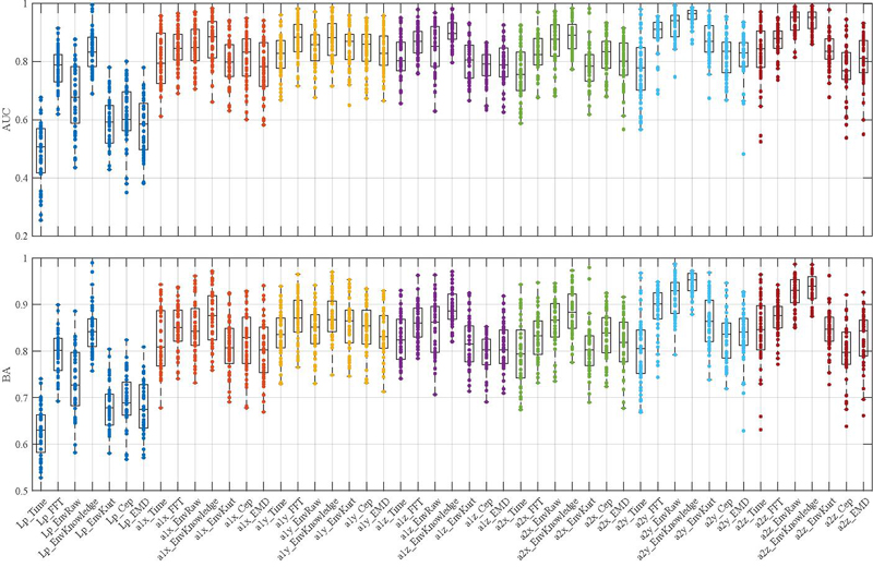
Distribution of AUC and BA values obtained by averaging the ML approaches across the load points. Each box represents the AUCs or BAs for a specific signal and signal processing technique (EnvRaw: Raw envelope, EnvKnowledge: Knowledge-based envelope, EnvKurt: Kurtogram-based envelope, Cep: Cepstrum).
At first, the results are treated as individual data points within a distribution. These distributions are visualized as box plots in Figure 5.1. According to the box plots, it can be observed that an accelerometer is preferable to a microphone based on fault detection quality, provided no signal processing methods are applied. However, when choosing the knowledge-based ES analysis, results can be achieved that are approximately equivalent to those obtained with the application of accelerometers. Here too, considering the median and the load point-specific dispersion in the representation, it is evident that the envelope-based method in combination with a knowledge-based filter yields better results. The highest median AUC and medium BA, around 0.965 or 0.952, respectively, and the smallest dispersion ranges are achievable using this method and the accelerometer fixed to the test stand in the planar directions or, in particular, the y-direction (a2y). However, methods based on Kurtogram, Cepstrum, and EMD generally tend to deliver poorer results, even when compared to the raw spectrum-based method. It is also worth mentioning that the raw envelope-based method generally yields significantly worse results than the raw spectrum-based method when processing the microphone signal Lp, while showing similar or slightly better median performance when applied to the accelerometers.
For a more detailed examination of the load points and a deeper understanding of the sensors, only the approaches including the knowledge-based ES analysis and the raw spectrum analysis will be considered henceforth, as the latter does not require domain knowledge in the form of a suitable filter band. Moreover, AUC and maximum BA values are strongly correlated across the entire dataset (see Figure 11). Thus, only the AUC values are reported for the sake of clarity and conciseness.
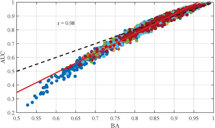
Figure 11 Correlation between AUC and BA values (Dashed line: Perfect correlation, Red line: Linear regression).
Figure 12 clearly confirms that knowledge-based ES analysis, when considering accelerometer 2, delivers higher AUC values across the entire operating range. It further shows that the rotational speed can have a significant impact on the quality of fault detection. While with this combination, the AUC only drops to a worst-case value of 0.862 at 400 rpm, values of 0.716 occur using the knowledge-based ES analysis applied to accelerometer 1 in the y-direction, and values of 0.620 occur using the microphone and the raw spectrum-based method. When using accelerometer 1 and the raw spectrum, there are partially opposing effects, as higher rotational speeds result in lower AUC values, especially at large swivel angles (BLs 5 to 8). However, the effect of BL on fault detection is not as apparent and necessitates a more detailed examination using the FPR assuming a TPR of 0, and the TPR assuming a FPR of 0. Figure 13 shows that the knowledge-based ES analysis tends to yield higher TPR values and lower FPR values at smaller swivel angles, although there are outliers. In this context, it is important to emphasize that the FPR can increase rapidly when the TPR is 0, especially if a single faulty unit does not exhibit truly anomalous behavior. If the goal is to avoid falsely detecting good units (see TPR), higher rotational speeds remain essential for robust fault detection. In particular, in these scenarios, the superiority of the knowledge-based ES analysis becomes evident.
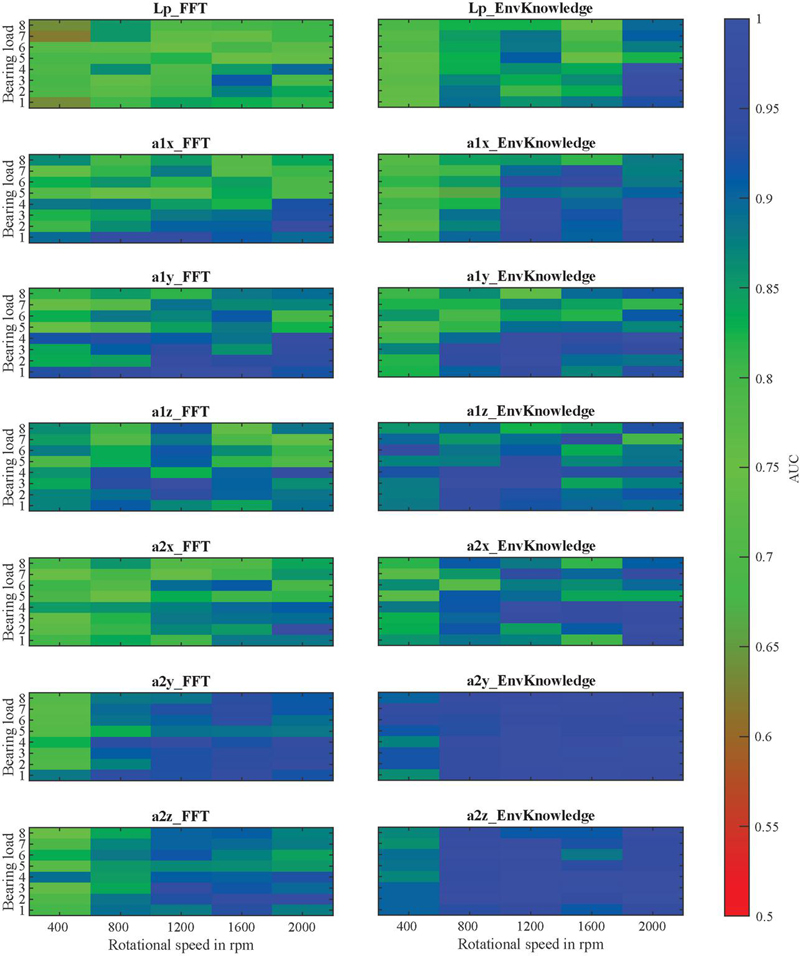
Figure 12 AUC values obtained by averaging the models depending on the load point.
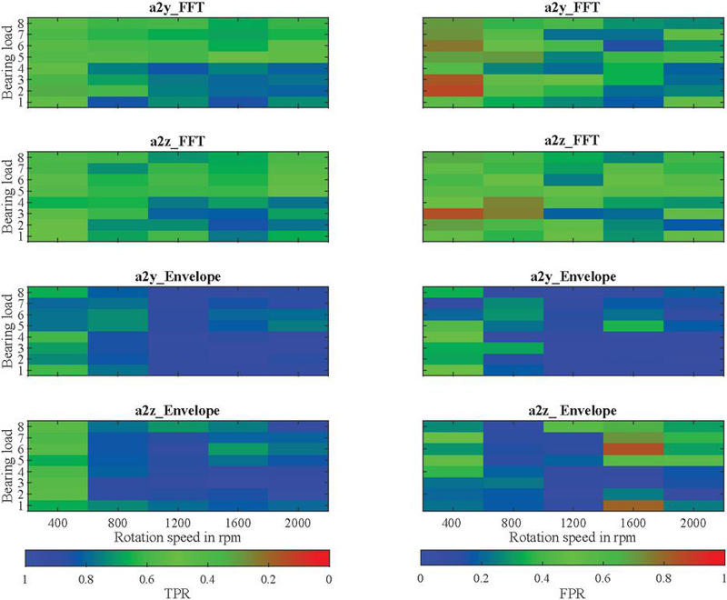
Figure 13 TPR (left) and FPR (right) values obtained by averaging the models depending on the operating condition.
A summary of the maximum AUC and BA values and TPR, as well as the minimum FPR values for the different sensors, is provided in Table 7 with corresponding signals, signal processing methods and load points. The knowledge-based ES analysis delivers the best values regarding the microphone and accelerometer 1. It is worth noting that, although the microphone metrics are superior to those of the accelerometers under optimal conditions, the results are not particularly robust across different load points. In this context, the reported load point LP36 (2000 rpm, BL4) should be considered a positive outlier. A similar observation holds for the raw ES analysis, which yields the best results for accelerometer 2 but does not provide stable performance across load points, as illustrated in Figure 5.1. This is particularly relevant since, in addition to systematic load point-related influences, stochastic variations in the feature space distributions also occur. In general, however, minimal swivel angle or displacement leads to the best anomaly detection performance, regardless of the sensor used.
Table 7 Best performance metrics achieved for each sensor type. The table displays the maximum Area Under the Curve (AUC), Balanced Accuracy (BA), and True Positive Rate (TPR), alongside the minimum False Positive Rate (FPR), identified across all tested load points and signal processing methods. The specific configuration (load point, signal, and signal processing method) that yielded this optimal result is indicated for each case
| Sensor | Metric | Value | Load Point | Signal | Signal Processing |
| Mic. | AUC | 0.995 | 2000 rpm, BL 4 | Lp | knowledge-based ES analysis |
| BA | 0.990 | 2000 rpm, BL 4 | Lp | knowledge-based ES analysis | |
| TPR | 0.976 | 2000 rpm, BL 4 | Lp | knowledge-based ES analysis | |
| FPR | 0.033 | 2000 rpm, BL 4 | Lp | knowledge-based ES analysis | |
| Acc. 1 | AUC | 0.987 | 2000 rpm, BL 4 | a1y | knowledge-based ES analysis |
| BA | 0.971 | 2000 rpm, BL 2 | a1x | knowledge-based ES analysis | |
| TPR | 0.938 | 1200 rpm, BL 3 | a1z | knowledge-based ES analysis | |
| FPR | 0.078 | 2000 rpm, BL 2 | a1x | knowledge-based ES analysis | |
| Acc. 2 | AUC | 0.994 | 2000 rpm, BL 3 | a2y | raw ES analysis |
| BA | 0.987 | 2000 rpm, BL 3 | a2y | raw ES analysis | |
| TPR | 0.971 | 2000 rpm, BL 3 | a2y | raw ES analysis | |
| FPR | 0.033 | 2000 rpm, BL 2 | a2y | raw ES analysis |
5.2 Evaluation of Machine Learning Approaches
To gain a deeper insight into the performance of individual models for anomaly detection, it is crucial to compare their metrics rather than relying on the mean values as previously considered. The distributions, which arise from different load points, reveal that no definitive general statement regarding performance can be made when varying scenarios for data collection and processing are taken into account, as illustrated in Figure 14. Using the IF (red), the median values for the metrics obtained from applying the raw spectrum-based method to the signals from accelerometer 2 are inferior compared to those obtained using the OC-SVM (blue) and the LOF (yellow). However, an analysis of the metrics derived from the knowledge-based ES analysis presents a different picture, with the OC-SVM yielding poorer median values and exhibiting significantly more variability depending on the load points. Particularly in the lower plot of Figure 14, it becomes evident that the variability for signal a2y and the knowledge-based ES analysis is considerably smaller, although the FPR can generally vary widely with respect to variable load points.
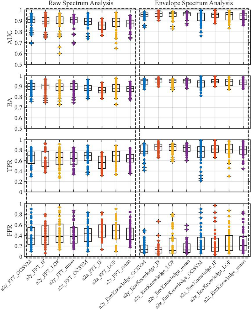
Figure 14 Metrics distributions for every single model across the load points.
Given that the different models incorporate distinct concepts for anomaly detection, it is prudent to examine the correlations between the individual models in greater detail. Figure 15 depicts the AUC values of the models for the previously analyzed signals and signal processing methods. Compared to a perfect correlation (dashed line), the discrepancies between the IF and the other two models are apparent. A depiction with a linear regression (red line) is inadequate here, resulting in a lower Pearson Correlation of 0.67 and 0.75, respectively. In contrast, a value of 0.92 when comparing the OC-SVM and the LOF indicates a significantly more similar categorization of instances and detection of anomalies.
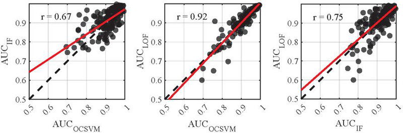
Figure 15 Correlation between the AUC values of the different models considering a2y and a2z (Dashed line: Perfect correlation, Red line: Linear regression).
6 Discussion, Limitations and Outlook
The experimental results indicate that detecting faulty roller bearings in a serial testing scenario is a non-trivial task, as the methods of data acquisition and processing, as well as the operating conditions, have a significant impact.
6.1 Current Findings
Sensor Choice and Transmission Path: The choice of sensors is critical, especially in the absence of domain knowledge and when only limited signal processing methods, such as raw spectrum analysis, are available. In TD, robust fault detection using a microphone is not feasible, as the generated features are subject to significant fluctuations. On one hand, the noise emissions from the test bench infrastructure interfere with the measurements. On the other hand, the transmission path through the air attenuates the noise emissions of the test object compared to direct SBN measurements. However, the superimposed noise emissions of the test bench predominantly affect lower frequency bands, as good results can still be achieved using a knowledge-based filter band within the ES analysis.
Measurement Repeatability: In contrast to systematic disturbances, the repeatability of the measurements with the available data is well verified. It is confirmed that the repeatability of accelerometer 2 on the test bench is higher, as no reapplication is necessary when testing a new unit. The sensor coupling and thus the transmission path of the SBN does not vary, unlike for accelerometer 1 on the unit, where the variation in sensor application is compounded by the general serial dispersion. Overall, it is evident that the advantage of the sensor being consistently applied outweighs the disadvantage of being further from the relevant noise source. This can be attributed to the rigid connection of the unit to the test bench.
Influence of Operating Conditions: The dependency of fault detection on operating conditions can also be attributed to hydraulic pulsations. Lower swivel angles result in reduced noise and hydraulic pulsations due to the lower inertia of the displaced fluid volume, leading to fewer noise disturbances that superimpose the SBN or ABN generated by the rolling bearing fault in the whole spectrum. The effects of rotational speed become particularly evident when high reproducibility, as seen with accelerometer 2, is achieved and noise disturbances are filtered out across a wide frequency range, as in the case of ES analysis. Lower rotational speeds result in reduced excitation of the rolling bearing and the transmission path to the sensor. Furthermore, the fixed measurement duration of 10 seconds affects the analysis differently at varying speeds. At lower speeds, this constant timeframe captures fewer pump revolutions, which weakens the statistical evidence of a repetitive fault pattern. Additionally, the resulting fixed frequency resolution can become too coarse to separate the fault’s harmonic components as they move closer together, leading to spectral smearing that obscures the characteristic signature. Consequently, there is a risk that minor faults may be masked by the background noise and the residual disturbances within this filter band. Conversely, high rotational speeds may have a more disruptive impact on accelerometer 1 if the adapter is induced to vibrate, which is application-dependent. Particularly in the z-direction, fault detection may be compromised at high rotational speeds.
Model Performance and Signal Processing: The superiority of the knowledge-based ES analysis, which is reflected in a high quality of fault detection with an AUC exceeding 0.9 across a wide range of load points when considering accelerometer 2, and even with suboptimal sensors such as the microphone, is based on the empirically determined filter band. This filter band characterizes a range where hydraulic pulsations are attenuated by the structure, and bearing resonances are pronounced. The raw spectrum-based method does not require such prior knowledge and can be generically applied to SBN or ABN signals. Anomalies or faults in a2y and the ES-based method in combination with a knowledge-based filter, for example, are more effectively detected by IF compared to the raw spectrum-based method. For the latter, the location of faulty data instances in the feature space favors better detection by the OC-SVM and the LOF, with a notable strong correlation between the latter two. Heuristic signal processing methods such as EMD offer no added value due to the dominance of hydraulic pulsations, and the cepstrum is also significantly influenced by the harmonics of the piston frequency and thus by hydraulic pulsations. The kurtogram is not a viable solution, as filter bands selected solely based on spectral kurtosis may be significantly influenced by the frequency peaks of hydraulic pulsations.
6.2 Future Work
Investigating Systematic Disturbances: It must be considered that additional acoustic disturbances, such as music, conversations, or other nearby machinery, could induce interference, which was not addressed in this study. It is plausible that the impact on SBN is lower due to the attenuation over the air transmission path, but this needs to be validated for the application, as disturbances can also be introduced through the structure, directly affecting SBN emissions. This also applies to other sources of interference, such as fluctuating fluid temperatures or system changes due to maintenance work. Thus, further research is crucial to determine the influence of these fluctuations, especially fluid temperature, on model performance. This research should investigate whether the impact of temperature variation is negligible compared to other variations (e.g., manufacturing tolerances), allowing models to leverage inherent fluctuations for robustness. If not, the need for conditional anomaly detection or transfer learning regarding varying temperatures or test bench modifications should be evaluated.
Enhancing Signal Processing: It is critical to question whether the empirically determined filter band remains consistent in a serial testing scenario where various variants and sizes of APUs are tested. To ensure robust fault detection, it would be prudent to determine the filter band automatically, for example, through machine learning. A data-driven approach could involve determining anomaly detection models in individual frequency bands and isolating anomalies on a band-specific basis. Furthermore, within the scope of signal processing, there is the potential to create enhanced envelopes (see Chapter 2) to calculate bands where hydraulic pulsations are minimized.
Advancing Machine Learning Approaches: It makes sense to identify the faults that are or are not detected by individual models and to refer to the configuration in the feature space, which, however, is not within the scope of this paper. Nevertheless, it should thus be verified whether robust frameworks for fault detection can be constructed using an ensemble of models, a common approach in machine learning. Whether majority voting (hard voting) or soft voting is more suitable needs to be verified. The use of relatively simple models is justified due to the limited data available, ensuring the development of generalizable models. If more data can be generated, this opens the possibility of employing more complex models based on deep learning, such as autoencoders or convolutional neural networks for anomaly detection. Particularly, the application of the latter in conjunction with the transformation of time series data into image representations could hold significant potential.
Addressing Shifts in Nominal Behavior: The underlying scenario of semi-supervised anomaly detection facilitates the learning of the nominal behavior of relevant units. In serial testing processes with low variant diversity and high production volumes, model training can be effectively conducted using historical data. However, if the nominal behavior changes over time, this poses a challenge in a semi-supervised scenario, as the robustness of the solution concerning other variants must be reassessed. In such cases, unsupervised methods for outlier detection without model training (see [7]), as well as transfer or cross-domain learning approaches such as siamese neural networks, could provide viable solutions.
7 Conclusion
This paper demonstrated a robust methodology for detecting roller bearing faults in APUs under realistic EoL testing conditions, successfully overcoming the key challenges of hydraulic noise and manufacturing-related serial dispersion. A core contribution was the novel experimental design, which simulated serial dispersion by systematically interchanging components. This provided a challenging and realistic dataset, validating that a data-driven pipeline can achieve reliable results in a high-variance industrial setting.
The findings reveal a clear and optimal solution: a single, fixed accelerometer on the test bench, combined with a knowledge-based envelope spectrum (ES) analysis, provides the most reliable fault detection. This optimized approach consistently achieved an AUC and BA above 0.9, with a best-case performance yielding a TPR of 97.1% at a zero FPR. The robustness of this setup stands in stark contrast to an APU-mounted accelerometer, which showed significantly higher performance variability across different load points. Furthermore, it is demonstrated that commonly used diagnostic methods like cepstrum analysis and kurtogram-based ES are counterproductive for this specific application.
In summary, this work provides a practical guideline for implementing a data-driven quality control system for the EoL testing of APUs. It shows that by combining smart sensor placement with targeted signal processing, it is possible to reliably identify units with faulty bearings even amidst significant background noise and manufacturing variations. This approach not only improves upon traditional methods but also paves the way for more automated and robust quality assurance in industrial manufacturing.
Acknowledgement
Acknowledgements are given to Bosch Rexroth AG for the financial support and the provision of the laboratory test bench. Further acknowledgements are extended to the test technicians and engineers for their support during the setup and commissioning of the experimental environment.
Overview of Reviewed Works
Table 8 provides a concise overview of the literature on vibroacoustic fault detection using ML or DL approaches.
Table 8 Overview of methods, models, operating conditions, and faulty components in reviewed works. (CWT: Continuous Wavelet Transformation, CNN: Convolutional Neural Network, kNN: k-nearest-neighbor, DT: Decision Tree, MED: Medium Entropy Deconvolution, FFT: Fast Fourier Transform, STFT: Short-Time Fourier Transform, WPT: Wavelet Packet Transform, EMD: Empirical Mode Decomposition, TSA: Time Synchronous Averaging)
| Work | Category | Signal processing | Learning paradigm | Model |
| [27] | 3 | CWT | Supervised | CNN |
| [33] | 4 | – | Supervised | CNN |
| [34] | 2 | FFT | Supervised | kNN, DT |
| [26] | 3 | STFT | Supervised | CNN |
| [28] | 3 | CWT | Supervised | CNN |
| [29] | 3 | CWT | Supervised | CNN |
| [30] | 3 | CWT | Supervised | CNN |
| [9] | 2 | WPT | Supervised | ANN |
| [31] | 3 | MED | Supervised | CNN |
| [19] | 2 | FFT | Supervised | Multiple |
| [32] | 3 | CWT | Supervised | CNN |
| [20] | 1, 2 | FFT, WPT, EMD | Supervised | SVM |
| [17] | 2 | FFT | Semi-supervised | PCA |
| [18] | 2 | WPT | Semi-supervised | PCA |
| [13] | 1, 2 | TSA, FFT | Supervised | Multiple |
| [12] | 1, 2 | FFT, CWT | Supervised | Multiple |
| [14] | 1 | – | Supervised | SVM, XGBoost |
| [27] | ABN | Single | Swash plate, slipper, center spring | |
| [33] | SBN, ABN | Few | Slipper, piston, valve plate | |
| [34] | SBN | Few | Valve plate | |
| [26] | SBN, pressure | Single | Slipper | |
| [28] | SBN, ABN, pressure | Single | Swash plate, slipper, center spring | |
| [29] | SBN | Single | Swash plate, slipper, center spring | |
| [30] | SBN | Single | Swash plate, slipper, center spring | |
| [9] | SBN | Single | Valve plate | |
| [31] | SBN | Single | Piston, cylinder, shaft | |
| [19] | SBN | Few | Port plate, slipper, cylinder | |
| [32] | ABN | Single | Swash plate, slipper, center spring | |
| [20] | SBN | Single | Piston | |
| [17] | SBN | Multiple | Slipper | |
| [18] | SBN | Single | General | |
| [13] | SBN | Few | Port plate, slipper, cylinder | |
| [12] | SBN | Few | Slipper, Roller bearing, cylinder | |
| [14] | SBN, pressure | Multiple | Slipper, valve plate |
Description of Manipulated Roller Bearings
Table 9 includes details about the location and size of the faults in the manipulated roller bearings.
Table 9 Detailed descriptions of the faults generated by abrasively manipulating roller bearings (RE: Rolling element, OR: Outer ring)
| Bearing | Location | Number | Largest Area [mm] | Maximum Depth [m] |
| 1 | RE | 5 RE | 21x4 | 40 |
| 2 | OR | 5 spots | 10x9 | 95 |
| 3 | OR | 1 spot | 33x5 | 400 |
| 4 | OR | 1 spot | 14x13 | 220 |
| 5 | OR | 1 spot | 33x4 | 95 |
| 6 | OR | 2 spots | 25x14 | 50 |
| 7 | OR | 1 spot | 33x40 | 300 |
| 8 | OR | 3 spots | 32x14 | 70 |
| 9 | RE | 6 RE | 14x7 | 78 |
| 10 | RE | 1 RE | 26x3 | 35 |
| 11 | RE | 3 RE | 8x2 | 45 |
| 12 | RE | 1 RE | 29x4 | 300 |
| 13 | RE | 7 RE | 24x6 | 380 |
| 14 | OR | 2 spots | 28x22 | 80 |
Dataset Analysis in Feature Space
The original dataset is partitioned according to Figure 8 into several data subsets (depending on load points and signals), and further divided into feature datasets based on the various signal processing techniques. Since many of these techniques inherently employ different feature sets, it is most effective to perform the analysis separately for each signal processing technique and sensor application. To visualize the resulting multivariate data, PCA is applied, reducing the dimensionality of the standardized data so that it can be represented in a two‐dimensional Cartesian coordinate system using the first two principal components (PCs). A detailed exposition of PCA is omitted here, as it does not form an integral part of the proposed methodology and reference is made to [44] instead. Note that the ML approaches operate in the PC space rather than the original feature space, and some information is lost due to the dimensionality reduction performed by PCA.
Due to the high number of feature datasets (40 x 7 x 7), a load-point-dependent analysis of the feature spaces is conducted first. Subsequently, an analysis is performed with regard to the different signal processing techniques and signals.
Load Point-dependent Analysis
To effectively analyze the influence of load points on the feature spaces, it is advisable to initially focus on a single signal and a specific signal processing technique. Therefore, the initial analysis is conducted based on the a2y signal and the raw spectrum-based method in feature space (). Despite this narrowing, 40 feature datasets still remain. To handle this complexity, it is useful to identify heterogeneous groups of feature datasets that are internally relatively homogeneous with respect to the different load points shown in Figure 6.
To derive representative feature datasets, the following procedure is used to form clusters of feature datasets by assessing the distributional similarity of them. As a first step, each matrix , representing the -th feature dataset (), is standardized column-wise across all available instances through z-standardization, which contrasts with the procedure used in the modeling pipeline, where standardization is performed based solely on the training data. This standardization, resulting in , reduces the influence of local fluctuations and enables a stable comparison across the feature datasets. Afterwards, the empirical covariance matrix for each feature matrix is computed as
| (23) |
which corresponds to the empirical correlation matrix and effectively captures linear relationships between features while being invariant to differences in scale. Afterwards, pairwise dissimilarity is quantified using the Frobenius norm between the covariance matrices:
| (24) |
where denotes the elements in the covariance matrices. Thus, the variance structure and inter-feature dependencies within each subset is captured, while absolute feature magnitudes do not have an impact. This is especially important regarding the presence of outliers and structural heterogeneity.
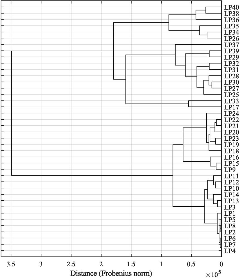
Figure 16 Dendrogram based on the distances between the covariance matrices of the individual load point-specific feature subsets. The hierarchical clustering is constructed in an agglomerative manner using the Ward method.
Based on the resulting dissimilarity matrix, K-means clustering (see [45]) is performed with a fixed number of 4 clusters. These clusters are also apparent when hierarchical clustering is performed based on the distances, which results in the dendrogram shown in Figure 16. While the clustering algorithm itself is not discussed in detail here, K-means is a well-established method for partitioning datasets into coherent and balanced groups based on pairwise distances. To extract representative feature subsets from each cluster, the medoid is selected, i.e., the sample within each cluster that minimizes the average dissimilarity to all other samples in the same cluster. This procedure yields the 4 representative feature subsets, which are linearly transformed using the PCA and illustrated in the PC space in Figure 17. However, one could also argue that there are two clusters of feature subsets (see Figure 16) which can primarily be attributed to rotational speeds up to and including 1200 rpm, and above that.
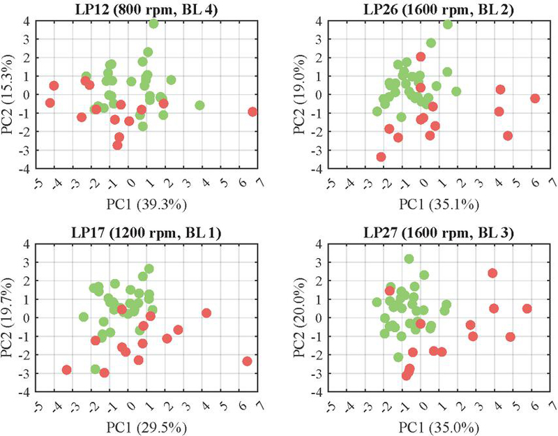
Figure 17 Representative feature subsets with healthy (green) and faulty instances (red) for different load points in the two-dimensional PC space using the raw-spectrum-based method on a2y.
As shown in Figure 17, it becomes apparent that the separation between healthy and faulty units is particularly less distinct within the first cluster of load point-specific feature subsets, i.e., generally at rotational speeds below 1200 rpm. Only a single faulty instance exhibits a clearly discernible distance from the cluster of healthy instances. In contrast, especially at LP26 and LP27, or within their corresponding clusters, several distinctly distant faulty instances can be observed, which are reflected in a larger first PC. However, there are always at least two faulty instances, that are not distinguashibly from healthy instances based on their location in the PC space It must be noted, however, that the first two PCs together explain only up to approximately 55% of the variance, and thus of the information contained in the respective feature subset datasets.
Signal Processing-related Analysis
As previously mentioned, the application of the signal processing techniques presented is associated with different feature spaces, since they are partially executed in different domains and also vary in terms of feature definitions. Nevertheless, PCA enables the transformation of these feature subets into an abstract, latent representation within a standardized PC space, thereby allowing for a comparable analysis across methods. To evaluate the signal processing techniques, the previously analyzed unit LP27 is revisited, and the signal a2y from the accelerometer 2.
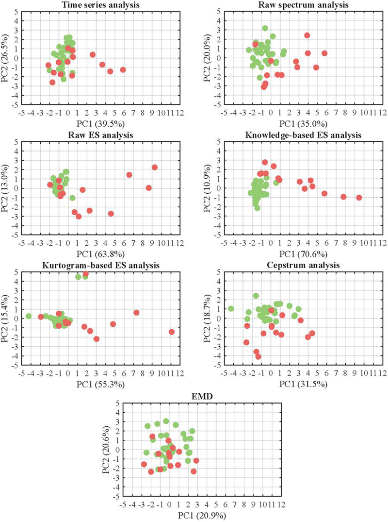
Figure 18 Feature subsets derived from different signal processing techniques with healthy (green) and faulty instances (red) in the two-dimensional PC space considering LP27 and a2y
As shown in Figure 18, the time-domain-based analysis results in only four faulty instances clearly emerging as outliers when considering the first two PCs, which, however, explain only about 55% of the variance in the corresponding feature subset. A more distinct separation between healthy and faulty instances is observable when using both the raw spectrum and raw ES-based approaches, with similar behavior noted in the cepstrum analysis. Particularly when applying the knowledge-based ES analysis, a large portion of faulty instances is distinctly separated from the bulk of healthy instances. This separation also accounts for the high proportion of variance explained by PC1. In contrast, for the Kurtogram-based method, some outliers are revealed to be healthy instances, although many faulty instances show significant distances from the remaining population. The EMD-based method exhibits very limited discriminative power between healthy and faulty instances, with the first two PCs explaining only slightly more than 40% of the total variance. This is generally indicative of a feature dataset heavily influenced by random noise, lacking systematic structures that could be attributed to faulty behavior.
References
[1] S. Haug. Ganzheitliche Optimierung einer Axialkolbenpumpe durch bedarfsangepasste Entlastung tribologischer Kontakte. KIT Scientific Publishing, Band 95, Karlsruhe, 2022.
[2] P. C. Palavicino, B. Sarlioglu, D. Bobba, W. Lee and T. Minav. Electrification of hydraulic systems using high-efficiency permanent magnet motors. 12th International Fluid Power Conference, Dresden, 2020.
[3] M. Tiboni, C. Remino, R. Bussola and C. Amici. A Review on Vibration-Based Condition Monitoring of Rotating Machinery. Applied Sciences, 12(2), 2022.
[4] C. Xiao, H. Tang, Y. Ren, J. Xiang and A. Kumar. A fault frequency bands location method based on improved fast spectral correlation to extract fault features in axial piston pump bearings. Measurement, 171, 2021.
[5] R. B. Randall and J. Antoni. Rolling element bearing diagnostics – A tutorial. Mechanical Systems and Signal Processing, 25:485–520, 2011.
[6] M. Bengtsson and G. Lundström. On the importance of combining “the new” with “the old” – One important prerequisite for maintenance in Industry 4.0. Procedia Manufacturing, 25:118–125, 2018.
[7] K. Hendrickx, W. Meert and Y. Mollet. A general anomaly detection framework for fleet-based condition monitoring of machines. Mechanical Systems and Signal Processing, 139, 2020.
[8] J. Bonart and W.-G. Drossel. Entwicklung einer End-of-Line Körperschallprüfmethodik für hochintegrierte elektrifizierte Antriebstopologien. Wissenschaftliche Scripten, 2024.
[9] J. G. M. Lázaro and C. B. Pinilla. A methodology for detection of wear in hydraulic axial piston pumps. International Journal on Interactive Design and Manufacturing, 14:1103–1119, 2020.
[10] S. Gaugel, B. Wu, A. Anand and B. Wu. Supervised Time Series Segmentation as Enabler of Multi-Phased Time Series Classification: A Study on Hydraulic End-of-Line Testing. IEEE 21st International Conference on Industrial Informatics (INDIN), 2023.
[11] J. Du, S. Wang and H. Zhang. Layered clustering multi-fault diagnosis for hydraulic piston pump. Mechanical Systems and Signal Processing, 36:487–504, 2013.
[12] T. Torrika. Bewertung von Analyseverfahren zur Zustandsüberwachung einer Axialkolbenpumpe. RWTH Aachen, 2011.
[13] P. Casoli, M. Pastori, F. Scolari and M. Rundo. A Vibration Signal-Based Method for Fault Identification and Classification in Hydraulic Axial Piston Pumps. Energies, 12(5), 2019.
[14] S. Horn, A. Shorbagy, M. Lenz, S. Knoll, M. Winter and J. Weber. Causal Condition Monitoring for Axial Piston Pumps: Prediction of Different Faults under Variable Operating Conditions. 2024 International Maha Fluid Power Conference, West Lafayette, 2024.
[15] S. Horn, A. Shorbagy, M. Lenz, S. Knoll, M. Winter and J. Weber. Economic Fault Detection for Axial Piston Pumps Under Variable Operating Conditions. International Journal of Fluid Power, 26(2), 2025.
[16] M. Christ, N. Braun, J. Neuffer, A. W. Kempa-Liehr. Time Series FeatuRe Extraction on basis of Scalable Hypothesis tests (tsfresh – A Python package). Neurocomputing, 307:72-77, 2018.
[17] O. Gnepper, H. Hitzer and O. Enge-Rosenblatt. Predictive Diagnosis in Axial Piston Pumps: A Study for High Frequency Condition Indicators Under Variable Operating Conditions. International Journal of Prognostics and Health Management, 14(1), 2023.
[18] L. Siyuan, D. Linlin and J. Wanlu. Study on Application of Principal Component Analysis to Fault Detection in Hydraulic Pump. Proceedings of 2011 International Conference on Fluid Power and Mechatronics, Beijing, 2011.
[19] P. Casoli, M. Pastori and F. Scolari. A multi-fault diagnostic method based on acceleration signal for a hydraulic axial piston pump. AIP Conference Proceedings, Modena, 2019.
[20] S. Xia, Y. Xia and J. Xiang. Piston Wear Detection and Feature Selection Based on Vibration Signals Using the Improved Spare Support Vector Machine for Axial Piston Pumps. Materials, 15(23), 2022.
[21] Y. Zhou, A. Kumar, C. Parkash, G. Vashishtha, H. Tang and J. Xiang. A novel entropy-based sparsity measure for prognosis of bearing defects and development of a sparsogram to select sensitive filtering band of an axial piston pump. Measurement, 203, 2022.
[22] A. Kumar, C. P. Gandhi, H. Tang, G. Vashishtha, R. Kumar, Y. Zhou and J. Xiang. Adaptive sensitive frequency band selection for VMD to identify defective components of an axial piston pump. Chinese Journal of Aeronautics, 35(1):250–265, 2022.
[23] Y. Zhou, A. Kumar, C. Parkash, G. Vashishtha, H. Tang, A. Glowacz, A. Dong and J. Xiang. Development of entropy measure for selecting highly sensitive WPT band to identify defective components of an axial piston pump. Applied Acoustics, 2023.
[24] A. Kumar, H. Tang, G. Vashishtha and J. Xiang. Noise subtraction and marginal enhanced square envelope spectrum (MESES) for the identification of bearing defects in centrifugal and axial pump. Mechanical Systems and Signal Processing, 165, 2022.
[25] P. Casoli, A. Bedotti, F. Campanini and M. Pastori. A Methodology Based on Cyclostationary Analysis for Fault Detection of Hydraulic Axial Piston Pumps. Energies, 11(7), 2018.
[26] Q. Chao, H. Gao, J. Tao, C. Liu, Y. Wang and J. Zhou. Fault diagnosis of axial piston pumps with multi-sensor data and convolutional neural network. Frontiers of Mechanical Engineering, 17(3), 2022.
[27] Y. Zhu, G. Li, S. Tang, R. Wang, H. Su and C. Wang. Acoustic signal-based fault detection of hydraulic piston pump using a particle swarm optimization enhancement CNN. Applied Acoustics, 192, 2022.
[28] S. Tang, Y. Zhu and S. Yuan. An improved convolutional neural network with an adaptable learning rate towards multi-signal fault diagnosis of hydraulic piston pump. Advanced Engineering Informatics, 50, 2021.
[29] S. Tang, Y. Zhu and S. Yuan. Intelligent fault diagnosis of hydraulic piston pump based on deep learning and Bayesian optimization. ISA Transactions, 129(Part A):555–563, 2022.
[30] Y. Zhu, L. Guangpeng, R. Wang, S. Tang, H. Su and K. Cao. Intelligent Fault Diagnosis of Hydraulic Piston Pump Based on Wavelet Analysis and Improved AlexNet. Sensors, 21(2), 2021.
[31] S. Wang and J. Xiang. A minimum entropy deconvolution-enhanced convolutional neural networks for fault diagnosis of axial piston pumps. Soft Computing, 24:2983–2997, 2020.
[32] S. Tang, Y. Zhu and S. Yuan. A novel adaptive convolutional neural network for fault diagnosis of hydraulic piston pump with acoustic images. Advanced Engineering Informatics, 52, 2022.
[33] Y. He, H. Tang, Y. Ren and A. Kumar. A deep multi-signal fusion adversarial model based transfer learning and residual network for axial piston pump fault diagnosis. Measurement, 192, 2022.
[34] N. Keller, A. Sciancalepore and A. Vacca. Demonstrating a Condition Monitoring Process for Axial Piston Pumps with Damaged Valve Plates. International Journal of Fluid Power, 23(2), 2022.
[35] C. Bienefeld, F. M. Becker-Dombrowsky, E. Shatri and E. Kirchner. Investigation of Feature Engineering Methods for Domain-Knowledge-Assisted Bearing Fault Diagnosis. Entropy, 25(9), 2023.
[36] Bearing Data Scenter. Accessed: Aug. 12, 2025. [Online]. Available: https://engineering.case.edu/bearingdatacenter.
[37] R. B. Randall. A history of cepstrum analysis and its application to mechanical problems. Mechanical Systems and Signal Processing, 3(19), 2017.
[38] B. Schoelkopf, J. C. Platt, J. Shawe-Taylor, A. J. Smola and R. C. Williamson, Estimating the Support of a High-Dimensional Distribution. Neural Computation, 13(7), 2001.
[39] P. Perera, P. Oza and V. M. Patel. One-Class Classification: A Survey. arXiv preprint, 2021.
[40] F. T. Liu, K. M. Ting and Z.-H. Zhou. Isolation Forest. 2008 Eighth IEEE International Conference on Data Mining, Pisa, Italy, 2009.
[41] fitcsvm. Accessed: Aug. 12, 2025. [Online]. Available: https://de.mathworks.com/help/stats/fitcsvm.html.
[42] M. M. Breunig, H.-P. Kriegel, T. N. Raymond and J. Sander. LOF: Identifying Density-Based Local Outliers. ACM SIGMOD Record, 29(2), 2000.
[43] O. Alghushairy, R. Alsini, T. Soule and X. Ma. A Review of Local Outlier Factor Algorithms for Outlier Detection in Big Data Streams. Big Data and Cognitive Computing, 5(1), 2021.
[44] S. Wold, K. Esbensen and P. Geladi. Principal component analysis. Chemometrics and Intelligent Laboratory Systems, 2(1), 1987.
[45] A. Ikotun, A. Ezugwu, L. Abualigah, B. Abuhaija and J. Heming. K-means clustering algorithms: A comprehensive review, variants analysis, and advances in the era of big data. Information Sciences, 622, 2023.
Biographies

Maximilian Romeser received his B.Eng. degree in Automotive Engineering from Ulm Technical University of Applied Sciences in 2021 and his M.Sc. in Automotive Engineering from the University of Stuttgart in 2023. Since 2023, he has been pursuing a Ph.D. at Ulm Technical University of Applied Sciences in cooperation with Bosch Rexroth AG. His research focuses on AI-based methods for fault detection in serial testing of axial piston units.

Reinhold von Schwerin received his Ph.D. in Computational Science from Heidelberg University and is now a professor for Data Science, Machine Learning and Artificial Intelligence at Ulm Technical University of Applied Sciences. Furthermore, he serves on the board of Directors of DASU – Transferzentrum für Digitalisierung, Analytics & Data Science Ulm which strives to strengthen the ties between academia and industry in the fields of Data Science, ML and AI.
International Journal of Fluid Power, Vol. 27_1, 175–224
doi: 10.13052/ijfp1439-9776.2716
© 2026 River Publishers