Experimental Generation of High-Frequency Oscillatory Flow in Hydraulic Systems
Faras Brumand-Poor*, Selim Karaoglu and Katharina Schmitz
RWTH Aachen University, Institute for Fluid Power Drives and Systems (ifas), Campus-Boulevard 30, D-52074 Aachen, Germany
E-mail: faras.brumand@ifas.rwth-aachen.de
*Corresponding Author
Received 05 October 2025; Accepted 01 April 2026
Abstract
Volumetric flow rate sensors are used in various technical applications. Therefore, it is interesting to use volumetric flow sensors that neither obstruct nor manipulate the flow to be measured nor are restricted to certain flow types and profiles. For this reason, the virtual volumetric flow sensor was developed. A test rig was constructed to validate this soft sensor, which can generate laminar, turbulent, steady, and unsteady flow rates. The dynamic part of the flow is generated by coupling three cylinders and operating a servo valve. In this work, an experimental hydraulic test platform capable of generating reproducible high-frequency oscillatory flow rates is investigated as an enabling system for validating a pressure-based virtual volumetric flow sensor. Two gain-scheduled PID control strategies are implemented to realize the required excitation profiles. Both controllers were intensively investigated on the test rig for various high-frequency scenarios, including pulsations up to 80 Hz. At 80 Hz, the direct controller achieves a normalized mean absolute error of 36.3% (including phase delay). After phase alignment, waveform fidelity corresponds to an nMAE of 10.1%, demonstrating suitability for high-frequency soft-sensor validation. The comparative results show that direct velocity control remains effective up to excitation frequencies of 80 Hz, while indirect position-based control becomes ineffective above approximately 40 Hz due to inherent phase delay. Eventually, the generated dynamic flow rate is utilized to demonstrate the high accuracy of the soft sensor for an oscillation of 20 Hz.
Keywords: High-frequency oscillatory flow, hydraulic test rig, gain-scheduled PID control, virtual flow sensor, experimental validation.
1 Introduction
Volumetric flow rate sensors are widely used in fluid power systems [1]. The knowledge of the existing volumetric flow in stationary and mobile hydraulic machines can be used to detect leakages and monitor component deterioration. In predictive maintenance, the determined volumetric flow and pressure can also be used to calculate performance, power loss, and thus the degree of utilization [1]. Currently, the volumetric flow rate in hydraulic lines is determined using invasive and non-invasive measurement methods. Invasive sensors are installed in the pipe from which the volumetric flow is to be determined. However, the invasive installation of such sensors changes the flow properties of the fluid flowing through, which is why this type of volumetric flow measurement can only be used for specific applications. Noninvasive sensor technology does not necessarily alter the fluid’s flow properties. Still, many of these measurement methods have specific requirements for the hydraulic line, such as transparency, or for the fluid itself, such as sufficient inductivity. In addition, specific measurement methods are limited to certain types of flow, such as turbulent, laminar, stationary, or transient.
To address this problem [1] developed a soft sensor that calculates the existing volumetric flow rate based on pressure data. Determining the volumetric flow rate based on pressure data in a pipe was made possible in the 19th century by establishing the Hagen-Poiseuille law. This equation calculates the volumetric flow based on the frictional pressure loss in a pipe. However, this equation is limited to laminar and static flows. Therefore, sudden changes in velocity due to oscillating flow movements and the resulting frequency-related changes in the velocity profile of the flow (see Richardson effect) are not considered. To be able to calculate the volumetric flow of laminar and stationary, but also compressible, unsteady, and transient flows based on pressure data for a straight-line pipe, an analytical model was derived as part of the virtual volumetric flow rate project [2, 1]. A test rig was built in the ifas test hall at RWTH Aachen University to validate this model [3, 4]. The test rig consists of three essential areas: The stationary flow source, the measuring line, and the oscillating flow source. The latter area of the test rig consists of the actuator components, cylinder coupling, and control valve. An oscillating flow rate can be set by controlling the cylinder coupling with a periodical velocity signal, i.e. sine wave. To validate the analytical flow rate sensor, it is essential to ensure a reproducible and precise oscillating flow rate is set. This work presents two gain-scheduled PID controllers for controlling a coupled cylinder system. In Section 2, current flow rate measurement methods and volumetric flow rate models are presented. Afterward, the virtual volumetric flow rate sensor is described, and a review of prior research dealing with controlling hydraulic cylinders is provided. The main contributions of this work are:
(i) the experimental demonstration of a coupled hydraulic cylinder system capable of generating reproducible oscillatory flow rates up to 80 Hz,
(ii) a comparative assessment of direct and indirect gain-scheduled PID control strategies with respect to their suitability for high-frequency excitation,
(iii) the validation of a previously developed pressure-based virtual volumetric flow sensor under controlled high-frequency flow conditions.
2 Transient Volumetric Flow Rate Determination
To contextualize the goal of this research, an overview of the existing flow rate measurement methods will be provided. After highlighting the shortcomings of current flow rate measurement methods, the theoretical groundwork for developing the analytical flow rate sensor will be laid. Finally, the analytical flow rate sensor itself will be discussed. Section 4 introduces the hydraulic test rig, the different control designs, and the investigated control test cases. Subsequently, the results are shown, and a discussion and outlook are provided. Section 4 presents the developed control strategies by introducing the hydraulic test rig and presenting the control design and the investigated test cases afterward. The results are presented in the subsequent Section, and a discussion and conclusion are provided.
2.1 Flow Rate Measurement
Several sensors are utilized to measure the volumetric flow rate in fluid power. One possibility to distinguish these sensors is their installation type: Non-invasive or invasive. Firstly, the non-invasive sensors exhibit one advantage of not disturbing the investigated flow. One measurement method is the electromagnetic approach utilizing Faraday’s law of induction. However, the investigated fluid must exhibit a specific conductivity of around 0.5 S/cm [5]. Standard hydraulic oils, such as HLP 46, have a conductivity of roughly pS/cm [6]. Ultrasonic flowmeters are another variant of non-invasive sensors. Their measurement principles rely on a pair of transducers mounted on the pipe, measuring the signal propagation time between both transducers, as outlined in reference [7]. One main drawback of this sensor is the assumptions of symmetry in the volumetric flow, which is inaccurate for turbulent pipe flows.
Regarding minimally invasive measurement methods, particle image velocimetry (PIV) is an advanced approach utilizing seeding particles in the investigated flow, which are illuminated by a laser to create a two-dimensional flow velocity profile. The particles are optically measured and used to determine the flow rate through the flow velocity [8]. A drawback of this approach is the usage of particles in the flow, which might alter the fluid’s properties due to contamination. A Coriolis flowmeter is also a minimally invasive method to compute the volumetric flow rate. The measurement relies on the Coriolis force, which is connected to the mass flow. The force is created by a fluid flowing through a bent tube, which is vibrating [5]. This approach is limited by the maximum measuring frequency, which is determined by the resonant frequency of the tube, which is around Hz [9].
The second main category of sensors is invasively installed, and many of them, such as turbine flow meters and positive displacement meters, compute the investigated flow rate by measuring the velocity of a moving volume. These sensors exhibit inaccuracy in dynamic flows because of the component’s inertia, resulting in a faulty tracking of fast flow changes [10]. Another approach is the creation of defined pressure drops by invasively installed components with a known hydraulic flow resistance. In the work of Kashima, the pressure drop is created by an orifice, and the volumetric flow rate is determined by the orifice equation [5]. However, these invasive installations change the investigated flow and result in a pressure drop, resulting in a less efficient system. Furthermore, the flow resistance for these components is often only valid for stationary flow, therefore being inaccurate for dynamic flow changes. Wiklung et al. investigated transient volumetric flows through differential pressure meters and concluded that these measurement methods become unreliable for volumetric flow rates above Hz [11]. Vortex flow meters are an invasive method that results in low-pressure drops and relies on tracking the Kármán vortex street. Due to its dependency on the Reynolds number (Re), its operation is constrained for laminar and low turbulent volumetric flow rates [12]. Hot wire anemometry (HWA) computes the volumetric flow rate by measuring the cooling rate of a heated wire inside the pipe. This method is accurate for high-frequency flow rates; however, it is bound to measure one point of the flow rate. The generation of a flow field is possible by installing several wires into the pipe, which eventually leads to an increased disturbance of the investigated flow.
In conclusion, flow rate sensors exhibit numerous drawbacks, ranging from inaccuracy for dynamic flow chances to high degrees of flow disturbance and requirements, which prohibit an application in standard fluid power systems.
2.2 Transient Volumetric Flow Rate Models
The prior sections underlined the limits of current sensors. In addition to flow measurements, numerous studies have been conducted on developing transient volumetric flow rate models. Brereton et al. developed a model for transient laminar pipe flows, which computes the volumetric flow rate based on the current and prior pressure gradients [13]. Following this research, Brereton presented an advancement that determines the volumetric flow rate to the centerline velocity [14]. Sundstrom et al. contributed significantly by refining the friction modeling for pressure-tie approaches, which substantially increased the volumetric flow rate computation accuracy of hydraulic systems [15]. Regarding transient volumetric flow rate determination based on differential pressure signals, Foucault et al. presented an approach using the potential of kinetic energy to compute laminar flow rates in real-time based on two coefficients [16]. New models have also been proposed for transient, turbulent pipe flows by García et al., who modeled the transient response of a turbulent flow and validated their model with experimental data [17]. The transition from turbulent to laminar flow rates was also investigated by García et al. by developing a mathematical model for the laminarization of the flow [18].
Urbanowicz et al. recently developed an analytical laminar water hammer model and validated their findings numerically and experimentally [19]. Further research by Urbanowicz et al. was conducted on deriving analytical models for wall shear stresses for the test case of water hammer events. These models contained quasi-steady and transient hydraulic resistance equations and exhibited a simplified representation and analytical representation [20]. Bayle et al. focused on wave propagation in water hammer events by modeling a rheological viscoelastic pipe and validating the findings experimentally [21]. Further research was done by them by utilizing the Laplace domain to derive a wave propagation model applicable to different boundary conditions in volumetric pipe flows [22].
2.3 The Virtual Volumetric Flow Rate Soft Sensor
The volumetric flow rate soft sensor aims to combat the disadvantages of existing flow rate measurement methods and ensure accurate flow rate determination for different kinds of flows. The soft sensor is developed by deriving an analytical model based on a variant of the Navier-Stokes equation and the general assumption of the conservation of mass. The derivation has been presented in previously published research [2, 1] and is out of scope for this work. Firstly, the soft sensor has been validated by results obtained by a parameter-distributed simulation model for unsteady pipe flow. Afterward, a test rig was constructed, and a successful validation with experimental measurement was conducted [3, 4]. The development of the test rig, especially the creation of hydraulic pulsation, was one of the primary investigations during the validation process. The main idea is to create an oscillating flow by the controlled movement of a three-component cylinder coupling, which is applied to both sides of the measurement pipe. Besides the cylinder coupling, a hydraulic pump provided a steady volumetric flow rate, and the cylinders’ movement created an unsteady volumetric flow rate. The test rig and the actual control of the cylinder coupling are presented in Section 4.
It is emphasized that the virtual volumetric flow sensor itself has been developed and theoretically derived in prior work [3, 4]. The present contribution does not extend the sensor model but focuses on its experimental validation under high-frequency oscillatory flow conditions. Although referred to as a soft sensor, the approach is physics-based rather than data-driven.
3 Control of Hydraulic Cylinders in Literature
This section reviews the existing literature on hydraulic cylinder control across various fields of application. Three selected studies are presented to provide a comprehensive overview of the research field of hydraulic cylinder control and contextualize this work’s results.
The first research by [23] examines the dynamics and stability of articulated steer vehicles (ASVs) with hydraulic steering systems. ASVs’ unique frame design resolves the conflict between high traction and maneuverability for off-road vehicles. However, the relative yaw motion of the two sections of the ASV frame, controlled exclusively by hydraulic cylinders, is heavily influenced by the hydraulic fluid properties, which reduce the effective stiffness of the cylinders. This can result in oscillatory yaw motion or “snaking behavior” when operating at higher speeds on paved roads. A control system was developed to address this issue, combining direct yaw moment control and force distribution to enhance ASV stability. The strategy incorporates feedforward and feedback compensatory controls, minimizing yaw oscillations while optimizing tire force distribution to maintain stability. The control system consists of two layers: the upper-level controller, which includes a feedforward gain and a feedback controller based on a linear quadratic regulator (LQR), and the lower-level controller, which converts torque values into longitudinal tire forces for each tire. Numerical simulations using sinusoidal steering at Hz demonstrated the efficacy of the proposed control system, which successfully eliminated snaking behavior and remained robust under varying tire cornering stiffness.
The following research by [24] addresses the challenges of position control in valve-controlled cylinder systems used in hydraulic excavators. The investigation considers nonlinearities such as dead zones, saturation effects, discharge coefficients, and friction, which are essential to ensure operational efficiency, safety, and adaptability in hydraulic applications. To tackle these challenges, a mathematical model was developed to capture the mentioned nonlinearities, including pilot and main valves, internal leakages, and flow characteristics. Two approaches for position control were compared: a traditional PID controller and the proposed system, in which PID parameters are auto-tuned using a Particle Swarm Optimization (PSO) algorithm. Depending on the pilot valve input voltage , the cylinder position is controlled. Simulation results were generated using step, ramp, and sinusoidal position references. For the sinusoidal input, the signal had an amplitude of approximately 500 mm and a frequency of Hz, demonstrating the effectiveness of the proposed control approach in managing nonlinearities.
The third and final research by [25] study explores high-performance position control of hydraulic servo systems (HSS), focusing on a two-link robotic manipulator actuated by hydraulic cylinder/servo-valve systems. Various control schemes were evaluated, including PID, Adaptive Inverse Dynamics Controller (AIDC), Adaptive Feedback Linearizing Control (AFLC), and Sliding Mode Control (SMC). To ensure comparability and consistency with the results of the subject of this research, only the results of the PID Control from [25] will be highlighted. Like [24], the PID control system adjusts the cylinder position based on the valve input signal . The evaluation involved actuating the two pistons of the hydraulic cylinder system with a cosine wave of amplitude 125 mm and frequency 0.33 Hz. The results demonstrated effective position control under these conditions.
Table 1 Overview of hydraulic control papers
| Control Settings | Quality Criteria | ||||
| Author | Control | Control Variable | Target Variable | ||
| [23] | LQR | 3.24 % | 257.47 | ||
| [24] | PSO-PID | 3.09 % | 24295.81 | ||
| [25] | PID | 0.26 % | 448.24 | ||
A quantitative approach is shown in Table 1 to guarantee a suitable basis for comparing all papers. The normalized mean absolute error () and the integrated time absolute error () are used as quality criteria.
The quality criteria is calculated by normalizing the mean absolute error of the reference signal and the measured signal (see Equations (1) & (2)).
| (1) | |
| (2) |
The quality criteria comprises the absolute error integrated over time (see Equation (3)).
| (3) |
4 Development of the Gain-Scheduling Control System Framework
This research aims to develop a control system that precisely sets the predefined velocity profiles for oscillating volumetric flow rate generation to validate the analytical flow rate sensor with the results from the test rig. For conclusive validation results of the analytical flow rate sensor, the control system must generate a variety of periodical velocity signals with different magnitudes of amplitude and frequency and be robust against different kinds of system and boundary conditions. These conditions include pressure differences within the test rig and mechanical properties of hydraulic components, especially of the actuator system.
4.1 The Hydraulic Test Rig
To validate the developed soft sensor, a hydraulic test rig was constructed and utilized to obtain experimental data. A comprehensive description of the test rig is provided in further research [3, 4]. The
The test rig can generate different volumetric flow rates, including laminar, turbulent, steady, and unsteady. The generation of the dynamic flow rate is done by moving two hydraulic cylinders and computing the dynamic flow rate by the displaced volume according to , with the velocity of the cylinder and the cross-sectional area . Pressure wave propagation and compressibility have to be considered to guarantee the accuracy of the determined reference volumetric flow rate. Firstly, to decrease the effect of compressibility, the operational pressure is set to be high, thus increasing the bulk modulus . Secondly, the reflection of the pressure waves is decreased by avoiding impedance change in the pipe. Installations along the pipe, which exhibit different cross-sectional areas, result in a change of impedance [26]. To address this, decreasing cross-sectional area changes and terminating the measurement pipe with a low-reflection line terminator (LRLT) are essential. An LRLT contains a cross-section adjustment mechanic like an orifice and a volume. By matching the orifice’s cross-section to the pipe’s characteristic impedance, the LRLT simulates an infinitely long pipe, effectively dissipating pressure waves in the termination volume and preventing reflections.
Figure 1 illustrates the hydraulic circuit used in the test rig.
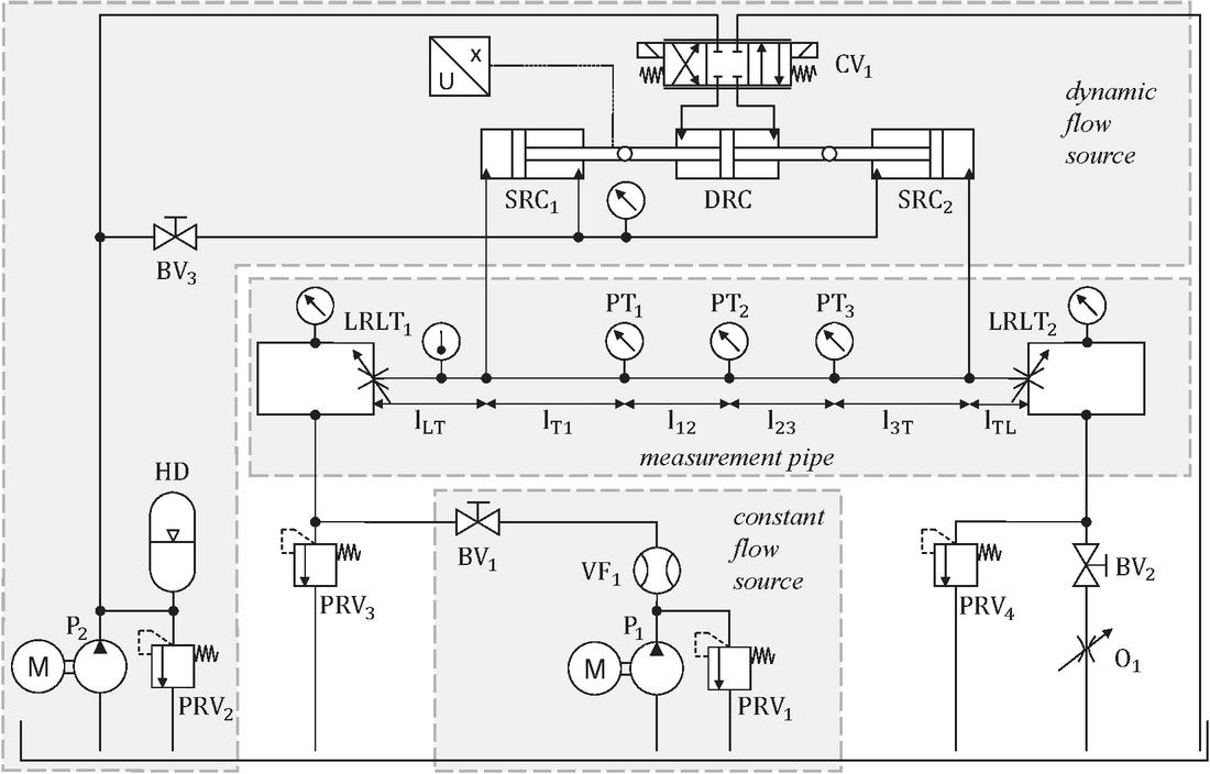
Figure 1 The hydraulic circuit of the test rig [4].
The primary component of the test rig is a measuring pipe, m in length, equipped with three designated points for pressure monitoring. The distances between the pressure transducers PT1 and PT2, and PT2 and PT3 are l12 m and l23 m, respectively. To minimize pressure wave reflections, LRLT1,2 are installed at both ends of the pipe, with each LRLT placed lLT = lTL m from the nearest T-junction. Additionally, an adjustable orifice, O1, is incorporated to regulate the pressure within the pipe, effectively reducing compressibility effects.
On the steady flow side connected to LRLT1, the system comprises a hydraulic pump (P1), a pressure relief valve (PRV1), and a volumetric flow sensor (VF1). The dynamic flow source, located on the opposite side, integrates a double-rod cylinder (DRC) driving two single-rod cylinders (SRC1,2) to generate fluctuating volumetric flows. The T-joints linking the measurement pipe to the dynamic flow source are situated at lT1 m from PT1 and l3T m from PT3, ensuring adequate inlet and outlet zones.
A servo valve (CV1) controls the double-rod cylinder, modulating the flow’s amplitude and waveform to enable various operating scenarios. Piston velocity is monitored using a position sensor mounted on one of the rods. The dynamic flow system also features a second hydraulic pump (P2), a pressure relief valve (PRV4), and switching valves (SV3) configured to pre-pressurize the single-rod cylinders. This pre-pressurization helps balance forces generated by the pressure in the sensing pipe and reduces mechanical stress on the connections. A coupling mechanism between the single-rod cylinders ensures fluid volume constancy in the pipe, as the suction from one cylinder compensates for the displacement of the other.
The LRLT orifices are adjusted based on the mean volumetric flow rate, , supplied by pump P1, as described by Equation (4). Any deviation in the flow rate through the orifice from alters the characteristic impedance and introduces errors in flow rate estimation, particularly at higher frequencies [3]. Switching valves (SV1,2) enable the system to operate in oscillating or pulsating modes. In the pulsating mode, the mean flow rate, , is combined with a dynamic component, . The volumetric flow rate derived from pressure measurements is validated by comparing it to the experimental flow rate calculated as (see Equation 4).
| (4) |
The design of the test rig is depicted in Figure 2, with its main components identified. The LRLT1,2, encircled in red, are situated at either end of the measuring pipe, highlighted in orange. The coupled cylinders outlined in blue drive the oscillatory fluid motion required to produce the dynamic flow rate.
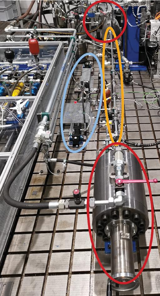
Figure 2 Picture of the constructed test rig [4].
A closer look at the dynamic flow rate source can be obtained from Figure 3.
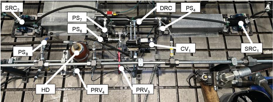
Figure 3 The actuator subsystem consisting of single-rod cylinders SRC1,2, double-rod cylinder DRC, pressure relieve valves PRV3,4, hydraulic damper HD & pressure sensors PS4,6,7,8.
4.2 The Control Design
The performance of control systems is confined and influenced by factors such as the properties of the selected controller type, the properties and quality of the measured signals, environmental and operational parameters, and the mechanical properties of real-world hardware. The control law defines the selection of the appropriate controller type.
The goal of the control system is to control the velocity profile of the cylinder coupling to validate the volumetric flow rate soft sensor. For a profound validation, the control system should handle different operating conditions. Operating conditions that are primarily influenced by the user of the test rig are the pressure in the hydraulic lines and the velocity and frequency of the velocity profile of the cylinder coupling. PID control was selected not as a novel control approach but due to its transparency, industrial relevance, and suitability for generating reproducible excitation profiles. The objective of the control system is not optimal tracking performance but reliable high-frequency excitation for experimental validation purposes. To still be able to combine the linear nature of the PID with the varying operating conditions of the hydraulic test rig, gain-scheduling will be deployed - the PID parameters will be changed at different frequencies and amplitudes of the desired velocity profile of the cylinder coupling.
The cylinder coupling is connected to a sensor that measures its position and velocity. Compared to the position, the quality of the velocity signal is relatively lower because of its higher noise (see Figure 4). To address this problem, two distinct approaches for PID control were developed:
Direct velocity control system: The closed loop controls depend on the filtered velocity reference and the measured velocity directly on the velocity of the cylinder.
Indirect velocity control system: The reference velocity signal is converted into a position signal. The closed loop controls depend on the converted position reference and the measured position, the position, and, by proxy, the velocity of the cylinder.
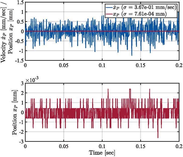
Figure 4 Position and Velocity signal noise with their standard deviations . The scaling was left untouched for the subplot above to show the qualitative magnitude of the noise of the velocity signal compared to the position signal . The lower subplot includes the scaled position signal.
The noisy velocity signal complicates the development of direct velocity control. To counter this, a first-order low-pass filter was chosen. The optimal filter coefficient is selected iteratively. With this proposed control structure, the desired velocity profile can be controlled without converting it to a position signal and without losing on dynamics. The control system can be seen in Figure 5.
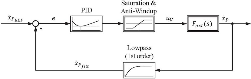
Figure 5 Block diagram of direct velocity control system. Unlike the indirect velocity control system, the reference cylinder velocity fed into the closed loop. The difference of the filtered cylinder piston velocity and reference results in the control error . From here, the controller determines the control variable , and the cylinder coupling is actuated by the control valve displacement, similar to indirect control. To close the control loop, a first-order transfer function with an iteratively selected filter coefficient will filter the measured cylinder velocity .
To design a control system that indirectly controls the velocity of the cylinder by its position, the velocity reference signal must be converted into a position signal. This process is straightforward because the velocity profile is a sine or cosine wave. If the velocity is inputted as a cosine wave, the integrated signal would result in a position sine wave. After that, a one-time closed control loop can be established (see Figure 6).
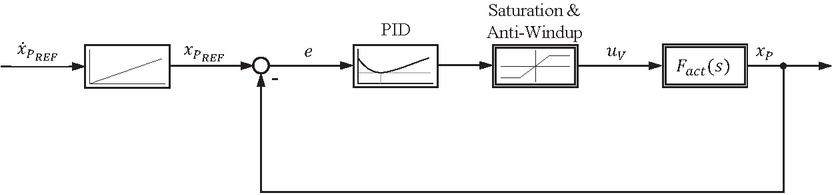
Figure 6 Block diagram of indirect velocity control system. The reference cylinder velocity is converted to the reference cylinder position . Subtracting the measured cylinder position results in the control error . The controller error is used to calculate the valve input . The control valve actuates the cylinder coupling, which results in the movement of the cylinder pistons . The control valve and the cylinder coupling are forming the actuator subsystem .
Reverting back to the start of this subsection, another confining factor is the mechanical properties of the test rig. when operating the test rig, a phenomenon of the so-called reverse backlash was registered after every change in the direction of the sinusoidal movement of the cylinder (see in Figure 7).
The problem with reverse backlash is very well known in applications for milling due to kinematic, mechanical, or thermal displacement [27]. The hydraulic test rig of the analytical soft sensor is not primarily strained by thermal or mechanical loads. Thus, the kinematics of the cylinder coupling would be the reason behind the reversed backlash phenomena. Possible causes are the movement play at the mounting points between the cylinder coupling and machine bed and the plays at the bearing connecting double- and single-rod cylinders (see in Figure 3).
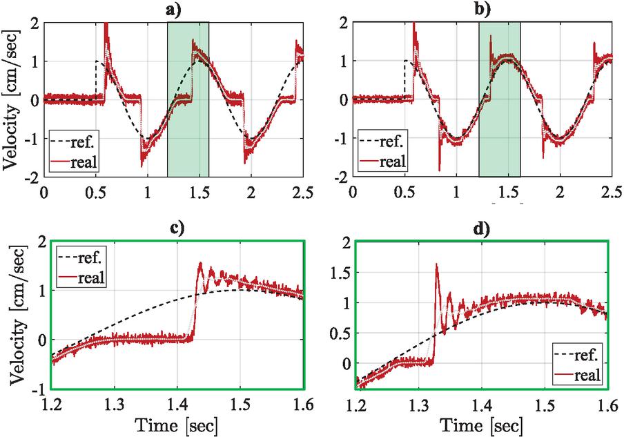
Figure 7 Controlled cylinder velocity with and without reverse backlash compensation at cm/sec and Hz: (a) without compensation, (b) with compensation, (c) zoom of (a), & (d) zoom of (b).
However, reverse backlash can be compensated reasonably uncomplicated by inputting an offset at every change of direction. The applied offset is constant and was determined empirically. It is triggered exclusively by direction reversal and does not adapt online. The purpose of the compensation is to suppress kinematic play rather than to improve tracking accuracy. The successful implementation of the compensation of reverse backlash can be seen in Figure 7.
As described at the beginning of this subsection, the two proposed control systems contain linear PIDs. The challenging part is combining linear control systems with a nonlinear plant. Hydraulics consists of different physical properties, namely viscosity, friction, flow profile, etc., which depend on the fluid’s velocity, temperature, pressure, and the mechanical properties of the parts transporting the fluid, such as pipes [26]. A gain-scheduled control system is proposed to use the advantages of linear control for a nonlinear plant. The PID controller’s gains are automatically adjusted depending on the plant’s requirements. Experiments were conducted to iteratively determine the PID gains at different frequency, amplitude, and pressure levels. Gain scheduling was implemented based on the excitation frequency of the reference velocity signal. PID parameters were identified experimentally at discrete frequency levels and interpolated linearly between operating points to ensure smooth parameter transitions without switching transients.
To quantify the effects of these values on the control performance, the quality criteria (normalized mean absolute error) and Phase Delay are used. The first grants knowledge of the overall accuracy of the control system, whereas the latter reveals the system’s behavior depending on time. The experiments show that the frequency negatively influences the overall control accuracy the most (see Table 2). While amplitude and pressure variations influence control performance, frequency was found to be the dominant factor. Therefore, subsequent investigations focus on frequency as the primary excitation parameter to characterize system bandwidth limitations relevant for soft-sensor validation.
Table 2 Control performance depending on different physical properties
| Variables | Phase Delay | |
| Amplitude | % | ° |
| Pressure | % | ° |
| Frequency | % | ° |
4.3 Test Cases
To quantify the stability and performance of the gain-scheduled control systems, experiments were conducted at different frequency levels of the reference cylinder velocity ranging from , , , , , , and 80 Hz with an amplitude of cm/sec (see in Table 3).
Table 3 The investigated Test Case from to 80 Hz at 20 cm/sec velocity amplitude. The results are calculated from data obtained within the first sine periods to maintain comparability. For Test Case 5, each control type includes two values because of different data frames (for explanation, see Section 5.5)
| Test Case | Frequency | Type | Phase Delay | |
| Test Case 1 | Hz | direct | % | |
| indirect | % | |||
| Test Case 2 | Hz | direct | % | |
| indirect | % | |||
| Test Case 3 | Hz | direct | % | |
| indirect | % | |||
| Test Case 4 | 20 Hz | direct | % | |
| indirect | % | |||
| Test Case 5 | 40 Hz | direct | % (%) | |
| indirect | % (%) | |||
| Test Case 6 | Hz | direct | % | |
| Test Case 7 | 80 Hz | direct | % |
The overall results of the Test Cases show that the direct control system outperforms the indirect control system significantly in all accounts. With increasing frequency, the direct control system still has more accuracy than its counterpart. At 40 Hz, the indirect control shows a sudden and substantial increase in . The reason is the delayed response of the indirect control after the defined sine periods. The indirect control system becomes unresponsive at frequencies higher than 40 Hz. In contrast, the direct control reaches frequencies as high as 80 Hz and maintains higher accuracy than the indirect control at 40 Hz (see Table 3).
5 Results
After the general overview of the performance of the control systems is shown, a detailed analysis of the control systems’ behavior at each frequency will follow. The same data frame of sine periods will be used for higher comprehensibility for all analyses. Besides the graphical analysis for quantification of the results, quality criteria like normalized Mean Absolute Error (), Integral Time Absolute Error (), and Phase Delay will be displayed.
5.1 Test Case 1
The results for Test Case 1 show good performance for direct as well as indirect control. Both control systems follow the reference accurately with almost no phase delay (see Figure 8).
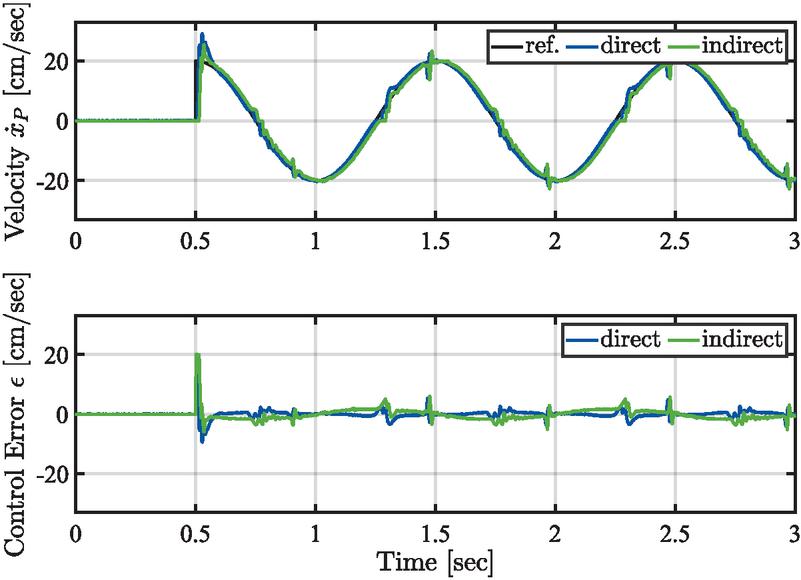
Figure 8 Velocity responses of direct and indirect control system for Test Case 1 at Hz.
The quality criteria reinforce the observations from Figure 8. Direct control is nearly twice as accurate and half as delayed as indirect control, reflected by all quality criteria (see Table 4).
Table 4 Results of Test Case 1
| Control Type | Phase Delay | ||
| Direct | % | ||
| Indirect | % |
5.2 Test Case 2
At Hz, the discrepancies between the controls are more observable. Because of the constant time delay, the phase delay of both controllers increases, enhancing the control errors. Still, both velocity profiles resemble the shape of the reference signal and are highly accurate (see in Figure 9).
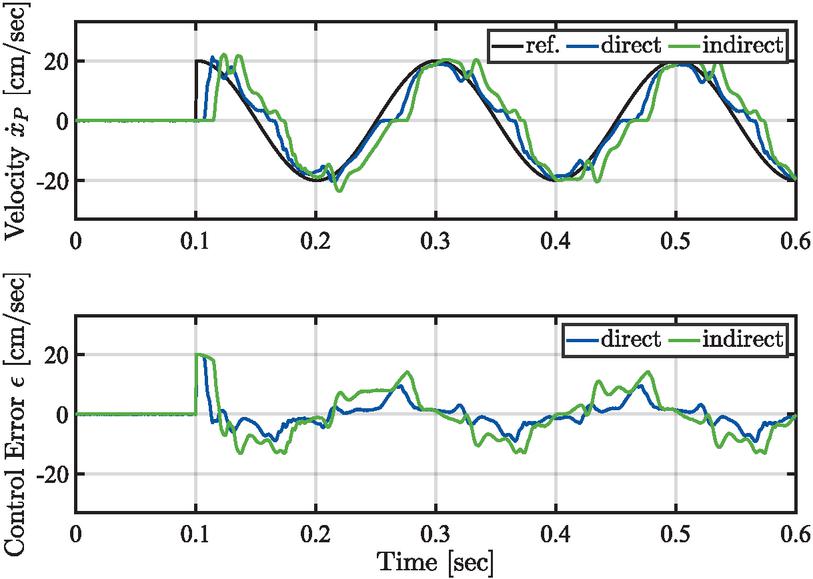
Figure 9 Velocity responses of direct and indirect control system for Test Case 2 at Hz.
Because of the higher phase delay, the accuracy of both controllers is influenced negatively. The increased for direct control by about % and for indirect control by about % (see in Table 5). Compared to one another, the of indirect control is twice as much higher as the of direct control. The difference in phase delay is 20 ° in favor of direct control.
Table 5 Results of Test Case 2
| Control Type | Phase Delay | ||
| Direct | % | ||
| Indirect | % |
5.3 Test Case 3
The observations from Test Case 2 are amplified for Test Case 3 – the constant time delay at Hz results in a higher control error, still higher for indirect control. But still, Figure 10 shows that the direct and indirect control velocity profiles resemble the reference signal. The phenomena of reverse backlash, which was addressed in Section 4.2, resurfaces at these higher frequencies (see in Figure 10).
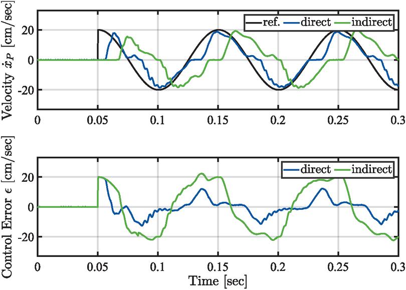
Figure 10 Velocity responses of direct and indirect control system for Test Case 3 at 10 Hz.
Table 6 reinforces the trend in the performance difference between direct and indirect velocity control. From to Hz, an increase of % for direct control is registered (about the same as from to Hz), whereas an increase of ca. % is present. At 10 Hz for indirect control is three times as much higher as for direct control. Phase delay is times higher, and is times as much for indirect control than for direct control (see in Table 6).
Table 6 Results of Test Case 3
| Control Type | Phase Delay | ||
| Direct | % | ||
| Indirect | % |
5.4 Test Case 4
At 20 Hz, the previous observations are significantly enhanced but still follow the same trend as the previous Test Cases. One characteristic behavior of all velocity signals, which was not expanded upon in the previous Test Cases, is the jittering effect. From to Hz, all velocity signals exhibit a jitter, whereas now, for 20 Hz, the velocity signal is smoothed out (see in Figure 11). The jittering at the lower frequencies may result from different factors: sensor signal processing, mechanical vibrations of the test rig, especially the cylinder coupling, and pressure waves. Presumably, the frequencies of these phenomena are lower than 20 Hz, hence the smoother velocity signals seen in Figure 11.
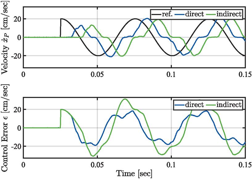
Figure 11 Velocity responses of direct and indirect control system for Test Case 4 at 20 Hz.
The quality criteria are amplified by the previous observations from Test Case 3 (see in Table 7. But presumably, because of the more prominent occurrence of phase delay, the distance between the quality criteria and from direct and indirect control decreases. At Hz, the difference for is approximately % and (see in Table 6. At 20 Hz, the differences increased for to % and for to (see Table 7). The difference in phase delay remains for Test Cases 3 and 4 at about .
Table 7 Results of Test Case 4
| Control Type | Phase Delay | ||
| Direct | % | ||
| Indirect | % |
5.5 Test Case 5
At 40 Hz, the first significant discrepancy between direct and indirect control is prevalent. The indirect control is not responsive within the first two and a half sine periods, whereas direct control is fully settled after one sine period (see Figure 12). When observing the control error signals of both control systems in Figure 12, it is apparent that contrary to the previous test cases, the control error of indirect control is significantly lower than that of direct control.
However, this is a direct result of the previously mentioned non-responsiveness of indirect control within the first milliseconds and also the delayed response of the direct control. The control error signal is the difference between the reference and measured signal. Because of the nature of a sine wave, which continuously has alternating signs, delayed responses are penalized heavier than no responses. The result can be seen in Figure 12. This is why a quantitative assessment of the control performance is also conducted. By normalizing the , the non-responsiveness of the indirect control should be penalized significantly, resulting in a higher for indirect control than for direct control.
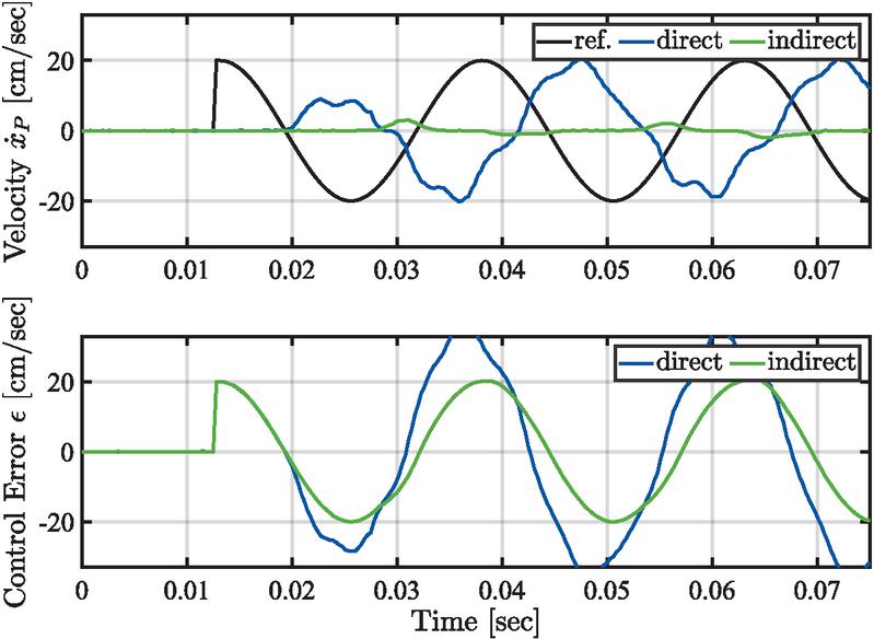
Figure 12 Velocity responses of direct and indirect control system for Test Case 5 at 40 Hz.
The extended data frame in Figure 13 shows that the indirectly controlled velocity signals fully settle after sec or about sine periods. This is a drastic decrease in dynamics compared to the response time of one sine period by direct control.
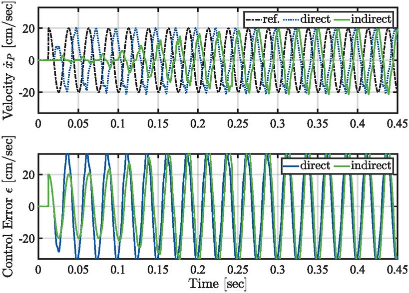
Figure 13 Extended view on direct and indirect control system velocity responses for Test Case 5 at 40 Hz.
Figure 13 showed that by including an extended data frame of the measurement data of Test Case 5 a more differentiated assessment on the performance of both control systems can be conducted. The quality criteria from Table 8 reflect this observation. The of direct control is shifted from % to %. In contrast, the of indirect control dropped from % to %. The high during settling time was averaged by including more data. The values of show this effect is reversed. The of direct control within the first sec of data is significantly higher than that of indirect control. Within the first seconds of the response time of both control systems, direct control’s integrated control error area is considerably larger than that of indirect control (see in Figure 12). When the indirect control is eventually settled, penalizes this late response substantially (see in Table 8).
Table 8 Results of Test Case 5
| Control Type | Data Frame | Phase Delay | ||
| Direct | Standard | % | ||
| Extended | % | |||
| Indirect | Standard | % | ||
| Extended | % |
5.6 Test Case 6 & Test Case 7
As described in Section 4.3, indirect control becomes unresponsive at frequencies higher than 40 Hz. Because of this, for Test Cases 6 & 7, only direct control results at Hz and 80 Hz will be presented. At Hz, direct control’s time delay and settling time are more prevalent. The control system responds after one-half of a sine period, and after one sine period, the system response is fully settled (see in Figure 14). Still, the velocity profile strongly resembles the reference velocity.
Similar observations can be made for the 80 Hz measurement. The only significant difference is the system delays at zero-crossing of the velocity signal (see in Figure 15).
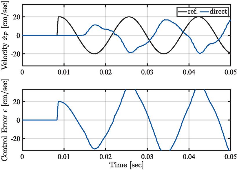
Figure 14 Velocity responses of direct and indirect control system for Test Case 6 at Hz.
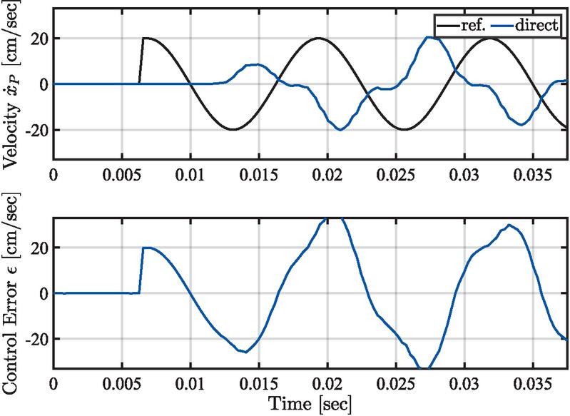
Figure 15 Velocity responses of direct and indirect control system for Test Case 7 at 80 Hz.
The quality criteria of both Test Cases can be obtained from Table 9. Following the observations from Figure 14 and Figure 15, the phase delay increased by about from Hz to 80 Hz. In contrast, the same trend is not present for . At 80 Hz, the is % lower than at Hz. The main contributing factor to the decrease in is that the velocity response shifts towards the next velocity reference amplitude with increasing phase delay. Thus, the maximum is reached at phase delay when the velocity response amplitude is at a half-sine wave period.
Table 9 Results of Test Case 6 & 7
| Test Case | Phase Delay | |
| Test Case 6 ( Hz) | % | |
| Test Case 7 (80 Hz) | % |
6 Discussion
The apparent degradation in control accuracy with increasing frequency is primarily driven by phase delay rather than waveform distortion. The Test Cases for 40 Hz and above also reinforced that velocity signals are more dynamic than position signals. On average, the time delay of direct control is msec, and indirect control is msec. The time delay strongly influenced the quality criteria. That is the main reason why, with increasing frequency, the control error and, consequently, increased.
As mentioned, the control systems were developed to control the cylinder coupling at a defined velocity profile. This velocity profile is essential for validating the analytical flow rate sensor. The correlation between the high accuracy of the sensor and the quality of the velocity profile only narrows down to not when but if the cylinder coupling fulfills the velocity magnitude and frequency. This means that if the velocity profile adequately resembles a sine wave, the control system fulfills its duty regardless of how much delay it comprises.
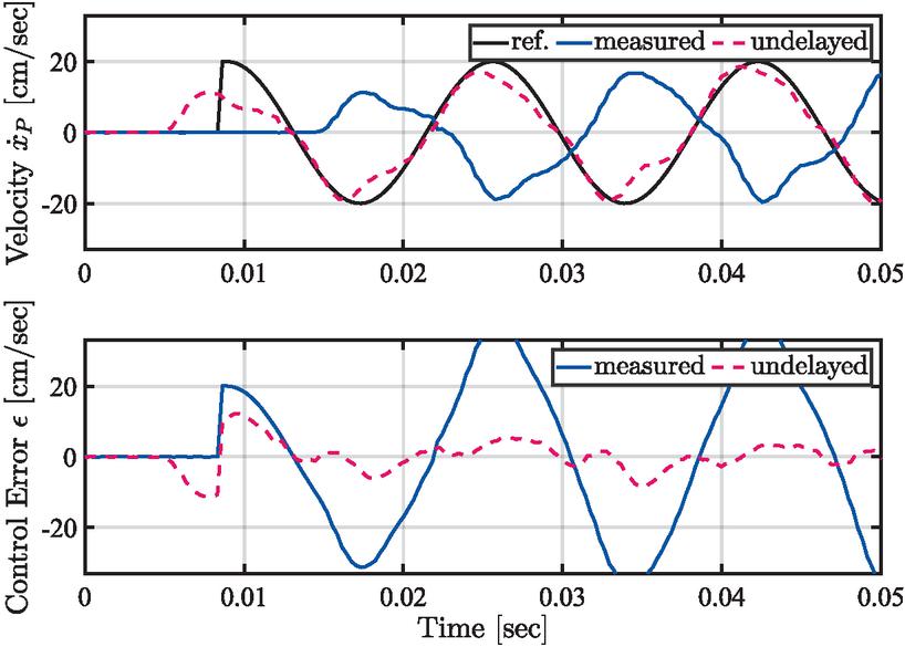
Figure 16 Delayed and undelayed Velocity responses of direct control for Test Case 6 at Hz.
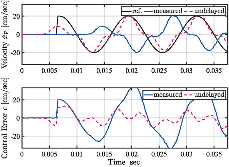
Figure 17 Delayed and undelayed Velocity responses of direct control for Test Case 7 at 80 Hz.
To investigate this premise, the cylinder velocity signals were post-processed. They were shifted to the same phase as the reference signals, eliminating the phase delay. Figures 16 and 17 show the post-processed velocity signals. The phase-aligned signals are shown for diagnostic purposes only and do not represent real-time control performance.
Table 10 reinforces that the control system delivers velocity profiles that adequately resemble a sine wave even at high frequencies.
Table 10 Results of Test Case 6 & 7 (with and without time delay)
| Test Case | Time Delay | ||
| Test Case 6 ( Hz) | With | % | |
| Without | % | ||
| Test Case 7 (80 Hz) | With | % | |
| Without | % |
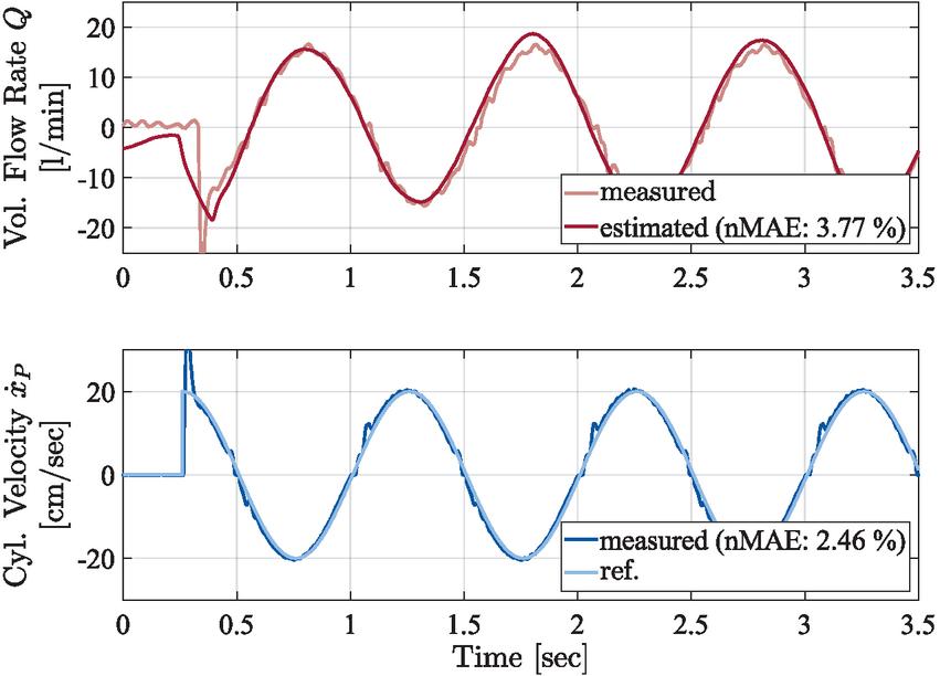
Figure 18 Demonstration of the previously developed pressure-based virtual volumetric flow sensor under controlled low-frequency excitation (1 Hz). The figure illustrates the suitability of the generated velocity profile for sensor validation rather than introducing a new sensor methodology.
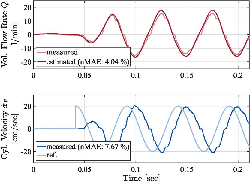
Figure 19 Demonstration of soft-sensor applicability under high-frequency excitation (20 Hz) enabled by the proposed experimental setup. The results serve to illustrate the usability of the generated oscillatory flow for validation purposes.
The main goal of developing velocity control systems was to enhance the validation of the volumetric flow rate soft sensor. Figures 18 and 19 show that up to 20 Hz with the developed control system, relatively high accuracy for the soft sensor can be achieved. Also, the previously investigated premise in this section is confirmed: For a proper validation of the soft sensor, only the quality of the controlled velocity signal is decisive, not the time and phase delay.
7 Conclusion
This research demonstrates the development and validation of two gain-scheduling control strategies. The use case generates an oscillating volumetric flow rate to conclusively validate the analytical flow rate sensor.
The experimental results demonstrate that direct and indirect control systems effectively manage oscillating volumetric flow rates. Each approach exhibits unique strengths in response to varying operational conditions. The results indicate that both control strategies achieve commendable performance up to 20 Hz. At frequencies higher than 40 Hz, the direct control excels reach up to 80 Hz with a remarkably low of % (see Table 9), whereas indirect control is not able to respond at such high frequencies. By adequately filtering the noisy velocity signal, the direct control system could assert itself against the indirect control system due to the higher dynamics of the velocity signal. Still, the indirect control proved to be a suitable alternative for use cases when the primary control variable is unavailable at low frequencies.
The results also showed that the accuracy of both control systems decreases with increasing frequency. The penalizes every deviation from measurement to reference. The results from Section 6 indicate that the primary source of error was the phase delay and not the response signal quality. Paired with the use case of the analytical flow rate sensor, the performance of the direct control system is suitable for the intended high-frequency excitation and soft-sensor validation task, achieving as low as % at Hz and % at 80 Hz (see in Table 10). In comparison, in current literature, compatible actuated hydraulic cylinder systems reached a between % to % at to Hz (see in Table 1).
The volumetric flow rate soft sensor itself addresses the limitations of conventional flow rate measurement techniques. A brief insight into the capabilities and performance of the soft sensor was given with the accuracy of flow rate prediction at and 20 Hz (see in Figures 18 and 19).
The purpose of Figures 18 and 19 is not to revalidate the sensor model itself but to demonstrate the practical applicability of the generated excitation profiles for experimental soft-sensor validation. The primary contribution of this work lies in the experimental demonstration of a hydraulic system capable of generating controlled high-frequency oscillatory flow suitable for validating a previously developed pressure-based virtual flow sensor. This advancement enhances the precision of oscillating flow generation and contributes to improved predictive maintenance strategies in hydraulic systems. As industries increasingly demand higher efficiency and reliability in fluid power applications, these findings offer valuable insights that can inform future research and practical implementations in this critical field.
Acknowledgement
The IGF research project 21475 N / 1 of the research association Forschungskuratorium Maschinenbau e. V. (FKM), Lyoner Straße 18, 60528 Frankfurt am Main was supported by the budget of the Federal Ministry of Economic Affairs and Climate Action through the AiF within the scope of a program to support industrial community research and development (IGF) based on a decision of the German Bundestag.
References
[1] F. Brumand-Poor, T. Kotte, E. Pasquini, and K. Schmitz. Signal processing for high-frequency flow rate determination: An analytical soft sensor using two pressure signals. Signals, 2024.
[2] F. Brumand-Poor, T. Kotte, E. Pasquini, F. Kratschun, J. Enking, and K. Schmitz. Unsteady flow rate in transient, incompressible pipe flow. Z Angew Math Mech. e, 2024.
[3] F. Brumand-Poor, M. Schüpfer, A. Merkel, and K. Schmitz. Development of a hydraulic test rig for a virtual flow sensor. In Proceedings of the Eighteenth Scandinavian International Conference on Fluid Power (SICFP’23), 2023.
[4] F. Brumand-Poor, T. Kotte, M. Schüpfer, F. Figge, and K. Schmitz. High-frequency flow rate determination - a pressure-based measurement approach. Preprints, 2024.
[5] Ayaka Kashima, Pedro Lee, and Mohamed Ghidaoui. A selective literature review of methods for measuring the flow rate in pipe transient flows. BHR Group - 11th International Conferences on Pressure Surges, pages 733–742, 01 2012.
[6] Y. Duensing, O. Richert, and K. Schmitz. Investigating the condition monitoring potential of oil conductivity for wear identification in electro hydrostatic actuators. Proceedings of the ASME/Bath 2021 Symposium on Fluid Power and Motion Control, 2021.
[7] B. Brunone and A. Berni. Wall shear stress in transient turbulent pipe flow by local velocity measurement. Journal of Hydraulic Engineering, 136, 2010.
[8] I. Grant. Particle image velocimetry: A review. Proceedings of the Institution of Mechanical Engineers, Part C: Journal of Mechanical Engineering Science, pages 55–76, 1997.
[9] M. Henry and M. Zamora. The dynamic response of coriolis mass flow meters: Theory and applications. Technical Papers of ISA, 454, 2004.
[10] Bernhard Manhartsgruber. Instantaneous liquid flow rate measurement utilizing the dynamics of laminar pipe flow. Journal of Fluids Engineering, 130(12), 2008.
[11] D. Wiklund and M. Peluso. Quantifying and specifying the dynamic response of flowmeters. Conference: ISA, 422:463–476, 2002.
[12] R. Mottram. Introduction: An overview of pulsating flow measurement. Flow Measurement and Instrumentation, 3:114–117, 1992.
[13] G. J. Brereton, H. J. Schock, and M. A. A. Rahi. An indirect pressure-gradient technique for measuring instantaneous flow rates in unsteady duct flows. Experiments in Fluids, 40(2):238–244, 2006.
[14] G. J. Brereton, H. J. Schock, and J. C. Bedford. An indirect technique for determining instantaneous flow rate from centerline velocity in unsteady duct flows. Flow Measurement and Instrumentation, 19(1):9–15, 2008.
[15] L. R. Joel Sundstrom, Simindokht Saemi, Mehrdad Raisee, and Michel J. Cervantes. Improved frictional modeling for the pressure-time method. Flow Measurement and Instrumentation, 69:101604, 2019.
[16] Eric Foucault and Philippe Szeger. Unsteady flowmeter. Flow Measurement and Instrumentation, 69:101607, 2019.
[17] F. Javier García García and Pablo Fariñas Alvariño. On an analytic solution for general unsteady/transient turbulent pipe flow and starting turbulent flow. European Journal of Mechanics - B/Fluids, 74:200–210, 2019.
[18] F. Javier García García and Pablo Fariñas Alvariño. On the analytic explanation of experiments where turbulence vanishes in pipe flow. Journal of Fluid Mechanics, 951:A4, 2022.
[19] Kamil Urbanowicz, Anton Bergant, Michał Stosiak, Adam Deptuła, and Mykola Karpenko. Navier-stokes solutions for accelerating pipe flow—a review of analytical models. Energies, 16(3):1407, 2023.
[20] Kamil Urbanowicz, Anton Bergant, Michał Stosiak, Mykola Karpenko, and Marijonas Bogdevičius. Developments in analytical wall shear stress modelling for water hammer phenomena. Journal of Sound and Vibration, 562:117848, 2023.
[21] A. Bayle, F. Rein, and F. Plouraboué. Frequency varying rheology-based fluid–structure-interactions waves in liquid-filled visco-elastic pipes. Journal of Sound and Vibration, 562, 2023.
[22] Alexandre Bayle and Franck Plouraboue. Laplace-domain fluid–structure interaction solutions for water hammer waves in a pipe. Journal of Hydraulic Engineering, 150(2), 2024.
[23] Y. Gao, Y. Shen, T. Xu, W. Zhang, and L. Güvenc. Oscillatory yaw motion control for hydraulic power steering articulated vehicles considering the influence of varying bulk modulus. IEEE Transactions on Control Systems Technology, 2019.
[24] Y. Ye, C.-B. Yin, Y. Gong, and J. Zhou. Position control of nonlinear hydraulic system using an improved pso based pid controller. Mechanical Systems and Signal Processing, 2016.
[25] T. O. Andersen, M. R. Hansen, H. C. Pedersen, and F. Conrad. On the control of hydraulic servo systems - evaluation of liinear and non-linear control schemes. In The Ninth Scandinavian International Conference on Fluid Power, SICFP’05, 2005.
[26] Katharina Schmitz and Hubertus Murrenhoff. Hydraulik, volume 002 of Reihe Fluidtechnik. U. Shaker Verlag, Aachen, vollständig neu bearbeitete auflage edition, 2018.
[27] L. Gan, L. Wang, and F. Huang. Adaptive backlash compensation for cnc machining applications. Machines, 2023.
Biographies

Faras Brumand-Poor received a bachelor’s degree in electrical engineering from RWTH Aachen University in 2017, a master’s degree in electrical engineering from RWTH Aachen University in 2019, and a master’s degree in automation engineering from RWTH Aachen University in 2020, respectively. He is a Group Leader of the research groups Fluids and Smart Systems and the Deputy Chief Engineer at the Institute for Fluid Power Drives and Systems at RWTH Aachen University. His research areas include machine learning, particularly deep learning, physics-based learning, fluid transmission lines, and virtual sensory systems.

Selim Karaoglu received a bachelor’s degree in mechanical engineering from TH Köln in 2021 and a master’s degree in mechanical engineering from TH Köln in 2023. Since 2024, he has been a Research Associate at the Institute for Fluid Power Drives and Systems (ifas) at RWTH Aachen University and a member of the Smart Systems research group. His research areas include the use of Asset Administration Shells for control system development, control engineering (both model-based and experimental), and the modeling of nonlinear system dynamics in electromechanical, thermodynamic, and hydraulic systems.

Katharina Schmitz studied mechanical and chemical engineering at RWTH Aachen University and Carnegie Mellon University, Pittsburgh (USA), and graduated in 2015 as Dr.-Ing. at RWTH Aachen University. Since 2018, she has been a full professor at RWTH Aachen University and director of the Institute for Fluid Power Drives and Systems (ifas). Additionally, she serves as Vice Dean of the Faculty of Mechanical Engineering at RWTH Aachen, a position she has held since 2020. Prof. Schmitz’s awards and honors include several best paper awards and 2023 IMechE Joseph Bramah Medal award.
International Journal of Fluid Power, Vol. 27_2, 1–34
doi: 10.13052/ijfp1439-9776.2726
© 2026 River Publishers