Using a Neural Network to Minimize Pressure Spikes for Binary-coded Digital Flow Control Units

Essam Elsaed*, Mohamed Abdelaziz and Nabil A. Mahmoud

Mechanical Department, Faculty of Engineering – Ain Shams University, Cairo, Egypt

E-mail: essam.elsaed@eng.asu.edu.eg; mohamed_abdelaziz@eng.asu.edu.eg; nabil_mahmoud@eng.asu.edu.eg

* Corresponding Author

Received 26 January 2019; Accepted 04 March 2020; Publication 14 March 2020

Abstract

A unique method of improving energy efficiency in fluid power systems is called digital flow control. In this paper, binary coding control is utilized. Although this scheme is characterized by a small package size and low energy consumption, it is influenced by higher pressure peaks and larger transient uncertainty than are other coding schemes, e.g., Fibonacci coding and pulse number modulation, consequently resulting in poor tracking accuracy.

This issue can be solved by introducing a delay in the signal opening/closing of the previous or subsequent valve, thus providing sufficient time for state alteration and valve processes. In a metering-in velocity control circuit, a feedforward neural network controller was used to create artificial delays according to the pressure difference over the digital flow control unit (DFCU) valves. The delayed signal samples fed to the controller were acquired through the genetic algorithm method, and the analysis was performed with MATLAB software.

The results display better overall tracking accuracy than do those of other methods. Although the system exhibits low accuracy at high acceleration demands, the proposed controller still slightly increased the accuracy compared under these conditions to traditional methods.

Keywords: digital hydraulics, speed control, pulse code modulation, pressure peaks, neural network.

1 Introduction

1.1 Addressing the Problem

In flow control using pulse code modulation (PCM), i.e., binary coding, particularly when shifting from a discrete flow value to another, pressure/flow peaks appear and affect the tracking accuracy due to transient uncertainty. This phenomenon occurs when the valves switch their states from ON to OFF, or vice versa. In other words, if a transition flow is demanded from 1Q to 2Q, the initial valve (V1) is closed, and V2 is opened by the digital flow control unit (DFCU; n = 2).

These tasks should occur immediately, but in reality, they take time due to valve dynamics, so two opposite possibilities can occur. First, if valves overlap for a short duration, the transient net flow (pressure peak) in this transition state is the summation of Q1 and Q2. This type of flow occurs because the V2 opening time is shorter than the V1 closing response time. Second, if valves underlap, in this temporary state, the transient net flow is zero. This type of flow occurs when the V2 opening time is longer than the V1 closing time. These transition states end when the valves successfully change their state to a stable steady state.

1.2 Summary of Previous Methods of Minimizing Pressure Peaks

Starting with (Linjama et al., 2002a), they retarded the closing of all valves with a fixed value to compensate for the slow opening process. Additionally, (Linjama et al., 2003) outlined the causes of pressure peaks are the load mass, system dynamics, and acceleration demands. Moreover, (Linjama et al., 2002b) defined the bounds of the opening and closing delays of the valves; however, the maximum system velocity was limited to decrease pressure peaks in certain conditions. Besides, the magnitude of the pressure peak was found to highly depend on velocity changes, the inertial load, and the closing behaviour of the valve. While (Laamanen et al., 2003) experimentally verified that uncertainty caused by viscosity changes is proportional to the flow rate. Furthermore, (Linjama and Vilenius, 2004) noted that delays also depend on pressure and temperature conditions. Moreover, they retarded the opening and closing of several valves with a specific constant value for each, and these values varied from 10 ms to 35 ms.

In a more specific study (Laamanen et al., 2004), the results based on two different pressure differences (2 and 8 MPa) were used to adjust the optimal delay compensation of every valve. The target of the controller was to have all the controlled valves switch their states simultaneously, consequently delaying the closing process. Regarding the methodology of acquiring these delayed values; in (Morel and Boström, 2007) research, closed-loop pressure and flow/velocity controllers were used. However, the valve delays were estimated from the open-loop responses of the tested system.

Another way of reducing, but not fully eliminating, pressure peaks is through employing electricity. Notably, (Laehteenmaeki et al., 2010) decreased the inherent valve delay from 35 ms to approximately 10 ms by boosting the valve with 36 V of DC. In addition, the results revealed that the valve size has an impact on delay variations. However, the difficulties associated with boosting the valve voltage above the recommended manufacturer value increase the possibility of valve malfunction and decrease the valve lifetime. Moreover, additional electric components and more advanced controllers are needed for boosting.

The first mathematical model of the pressure peak phenomenon related to PCM control was introduced and theoretically discussed by (Laamanen et al., 2005), but no proposed controller was presented to resolve this issue. The authors highlighted the negative effect of peaks on a hydraulic circuit due to inexact switching times and suggested that the most promising pressure peak minimization methods are switch time tuning methods and cost function-based controllers. Later, the same authors (Laamanen et al., 2007) suggested that the risk of pressure peaks formation is the highest in PCM coding, followed by Fibonacci coding, then pulse number modulation (PNM).

Another cause of pressure peaks is the poor repeatability of valve processes; consequently, (Ketonen et al., 2012) recommended that the switching time must always be slightly longer than the valve response time, because the random uncertainties associated with valve opening can cause large pressure peaks.

A key study (Linjama and Vilenius, 2007) classified uncertainties in a binary-coded DFCU into two types: steady state uncertainty and transient uncertainty, the former of which can be divided into two forms. First, steady state output (flow rate) uncertainty is due to the fuzzy effective opening of the valve. Second, step size (timing) uncertainty, which is equal to the sum of the uncertainties of all operating valves during state changing; for example, if a step input of 5Q is called, it cannot instantaneously occur, so a lag time passes before reaching this value. During a transition event – which includes the simultaneous opening and closing of valves – and due to variations in the response time, valves tend to overlap or underlap. Notably, pressure peaks appear in case of valves overlapping.

In conclusion, two main factors affect pressure peaks in transient states.

The first factor is related to the circumstances, such as a change in the operating pressure, temperature, fluid viscosity, or valve size. Variations in the operating pressure for different valve sizes will be investigated and compensated for, and these changes are modelled through hydraulic characterizations.
The second factor is randomness or inaccuracy (uncertainty) associated with the valve itself, which is beyond the scope of this study.

2 System Description and Dynamic Modelling

2.1 Preface: A Case Study

This study is based on the work performed by (Elsaed et al., 2017), who compared the energy efficiency of a DFCU using five on/off poppet valves (Hydraulics, 2018a) and a low-cost proportional valve (Hydraulics, 2018b) when implementing a metering-in hydraulic circuit. The comparison indicated the DFCU managed to achieve a 93% energy reduction over the proportional valve because the latter operates at a much higher pressure, although poor tracking performance was observed. The source of the highest portion of these fluctuations was DFCU dynamics and not the DFCU resolution (Elsaed et al., 2017). Moreover, decreasing the DFCU step size did not considerably reduce these deviations.

The hydraulic system shown in Figure 1 is comprised of a (ϕ32/16–1000) mm cylinder, a 4/3-way spool valve (Wadowice-WE6s12x), a relief valve (Oleoweb-VMDR40) with a maximum pressure set to approximately 20 bar, a pump (HYDURA PVQ-06), a motor unit (1.5 kW rated power) with a maximum delivery of 13.9 cm³/rev, a single DFCU (n = 5). The DFCU included five on/off solenoid direct-operated poppet valves (Hydraulics, 2018a), and the variable-load ranged from 0 to 1000 N.

The oil 30-W bulk modulus used was 1.7 GPa at atmospheric pressure, and this value was modelled as a variable according to the system pressure. One application of a dynamic model of fluid compression is to determine the fluid hammer effect in the system. In this case, the effect accounted for just 0.3 bar increase in the pressure.

The natural frequency of the system (ω_n) is 40 Hz, which is ten times the digital valve operating frequency.

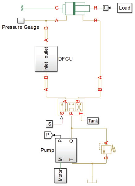
Figure 1 Developed near-real DFCU (n = 5).

2.2 Mathematical Equations

Velocity tracking is challenging in digital hydraulic valve systems when the velocity approaches the smallest possible value (Linjama et al., 2016); to address this issue, a hydraulic circuit with a low-speed range and a rated load speed (v_r) equal to 30 cm/s at a rated load (F_r) of 1000 N was developed.

The approach used was PCM with a DFCU (n = 5) due to the compact size and adequate flow steps in the approach. At n = 5, the velocity output has 31 steps ranging from 0.5 to 15.5 L/min. An orifice is attached to each valve of the DFCU to adjust the valve flow rates based on the PCM sequence of 1, 2, 4, 8, and 0.5 L/min; this is an ideal sequence that is difficult to achieve in reality. Orifice diameters of 0.85, 1.3, 1.8, 2.5, and 0.6 mm were selected for the on/off valves at a maximum load of 1000 N. The objective was to achieve the desired flow sequence with the minimal orifice differential pressure (ΔP_o). These orifices were modelled according to formula (1) (MathWorks, 2006).

Q = C_{d} \times A_{o} {(2 / ρ_{o})}^{1 / 2} \times {[Δ P_{o} / (Δ P_{o}^{2} + P_{c r}^{2})]}^{1 / 4}

(1)

The effective valve area was calculated using the valve performance curve from (Hydraulics, 2018a) and Equation (2) – a simplified form of Equation (1) – by assuming d = 0.8, ρ = 850 kg/m³, and ΔP_v = 2.4 × 10⁵ Pa at Q = 8 L/min, or 1.33 × 10⁻⁴ m³/s. Subsequently, the effective valve diameter is 3 mm.

Q = C_{d} \times A_{v} {[(2 Δ P_{v}) / ρ]}^{1 / 2}

(2)

Remarkably, the area ratios of the valves to orifices vary from 25 (smallest orifice) to 1.4 (largest orifice). These differences will significantly impact the formation of pressure peaks.

3 Controller Design

In the proposed system, the control objective is to regulate the speed of the payload. The utilized controllers are introduced below.

Feedforward controller design based on a steady state model: This controller controls the actuator speed by regulating the metered inflow through the DFCU and the cylinder load through a feedforward process.
Predictive control scheme based on a neural network: This approach reduces the transient system peaks by introducing a discrete variable-based artificial delay to the DFCU valves.

3.1 Feedforward Controller Design Based on a SteadyState Model

3.1.1 Controller configuration

The DFCU adjusts the inlet flow so that it balances the actuator velocity demand based on the load disturbance by adjusting the effective openings of the valves. The open-loop feedforward controller was used in a recent study by (Huova et al., 2013) in a 4-DFCU system; they experimentally obtained a high tracking accuracy with a reduction in energy consumption of (20–60)% at different loads compared to that of a proportional valve.

3.1.2 Controller governing equation

Based on the research of (Linjama et al., 2003), the governing formula for the proposed circuit is as follows (3).

u_{p} = (A_{A} \times v_{desired}) / [Q_{N, P 1} {[P_{s} - (F + A_{B} \times P_{B}) / A_{A}]}^{1 / 2}]

(3)

In this case, the calculated signal u_p is used to open a group of on/off valves. The signal u_p is rounded up and binarized to u_pi, i.e., 1, 2, 4, 8, or 0.5. Here, the system has only 32 states (including zero), as n = 5. Accordingly, the subsequent flowchart (Figure 2) demonstrates the controller procedures. Note that Equation (3) can be simplified by assuming that P_s is the gauge pressure prior to DFCU implementation and that P_B is the tank pressure, i.e., zero gauge.

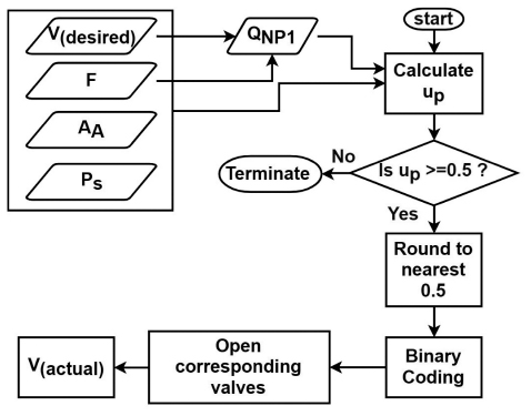
Figure 2 Feedforward control diagram of the DFCU (n = 5).

3.2 Predictive Control Scheme Based on a Neural Network

3.2.1 DFCU valve dynamics Inherent delay

A 2-position valve actuator was used to drive the on/off valves, and both the ON (50 ms) and OFF (50 ms) responses were modelled. Furthermore, the dynamics of the valves were modelled as a delay phase, a subsequent constant acceleration phase, and finally a constant velocity phase.

In this case, the valve opening and closing response times are similar; however, this is compensated by the difference in the hydraulic flow time, which is influenced by the corresponding hydraulic characteristics. Notably, the flow response is faster when opening a valve than when closing a valve. In other words, because the area ratios of valves to orifices vary from 25 to 1.4, as previously calculated, it is evident that a significant portion of the hydraulic resistance results from the orifices, not the valves. Consequently, any short extending stroke (opening valve) will pass a large part of the flow, while to stop the large fluid portion, a lengthy retracting stroke is needed (closing valve). It is therefore imperative to delay the opening of valves, such that the valve opening and closings processes occur as simultaneously as possible.

Table 1 shows the state transitions for the ramped input of a DFCU (n = 4) (where n = 4 provides a more straightforward example than n = 5).

Table 1 Valve delay conditions in ascending order based on the flow demand of a DFCU (n = 4)

Valves	DFCU (n = 4) Combinations
V1	1	0	1	0	1	0	1	0	1	0	1	0	1	0	1
V2	0	1	1	0	0	1	1	0	0	1	1	0	0	1	1
V3	0	0	0	1	1	1	1	0	0	0	0	1	1	1	1
V4	0	0	0	0	0	0	0	1	1	1	1	1	1	1	1

Net Flow	1	2	3	4	5	6	7	8	9	10	11	12	13	14	15

An analysis of Table 1 yields the following findings.

An induced delay is required only for valves opening under certain conditions, as represented by the grey blocks.
An artificial delay is needed whenever a state is changed from (2ⁿ⁻¹−1) to (2ⁿ⁻¹) (i.e., from 7 to 8), and vice versa. Because all valves contribute to this transition overlap for a short period.
In ascending order, V1 (step size of the DFCU n = 4) needs no delay because when shifting from a state where V1 is closed to a higher state flow, e.g., Q2 to Q3, the latter desired state is always the summation of the former state plus V1 (step size). Thus, when overlapping occurs, it is for the benefit of the system because this combination will result in the new demanded state. However, in ascending, unordered specific transition states (9 transition states in DFCU n = 4), i.e., (Q2 to Q5), (Q2 to Q9), (Q2 to Q13), (Q4 to Q9), (Q4 to Q11), (Q6 to Q9), (Q6 to Q11), (Q6 to Q13), (Q10 to Q13), the artificial delay values are necessary for the smallest valve (V1). These states occur when V1 is closed in the first state, while it is opened in the second one, and at least another valve is opened in the first state and is closed in the last.
Also, in ascending, unordered transition states, e.g., from Q1 to Q6 (corresponding to V1 to (V2 + V3)), the subsequent V2 and V3 opening signals must be delayed.
However, in descending transition states, whether it’s in order or not, as long as the valves shift from OFF to ON, they should be delayed at the opening. For instance, a transition from Q2 to Q1, V1 must be delayed, similarly, from Q9 to Q6, both V2 and V3 should be delayed. This is because, at least one of the valves that were opened in the first state will close in the second state. Therefore, the delay is required at the opening to prevent unwanted super positional flow.
For a ramped input, the first valve opening requires no delay because no transition has yet occurred.

For a DFCU with n = 5, the actual coding scheme used in this paper, the only difference is the step size is 0.5 L/min, and the maximum flow is 15.5 L/min. To apply these concepts, first, a Stateflow controller is constructed, as shown in Figure 3. V1 delay scheme is presented in the following flowchart, and slight changes in the configurations of other valves delay schemes were considered. To the best of the authors’ knowledge, no previous study has introduced a delay state-oriented technique, such as that described here. In other words, generally delaying the opening of valves at all state transitions, as previously shown in the literature, will not achieve an optimal solution.

Valve switching time

According to the information given by the manufacturer (Hydraulics, 2018a), the valve switching frequency (f) is 4 Hz. However, at steep trajectories, the controller orders the valves to switch rapidly to keep track of the reference. Therefore, a sort of switching regulator function is created to limit the operating frequencies of the valves. The working principle of this function (Figure 4) is to ensure a minimum of half period elapsed before changing the valve state, where T is the periodic time, i.e., 25 ms. In practical applications, it is recommended to limit the switching frequency of the valves to only 20% to avoid repeatability issues. In this research, a 5 ms sample time is used for delay compensation and the MATLAB solver.

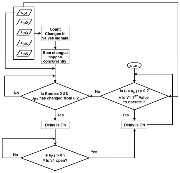
Figure 3 Delay implementation flowchart (with valve 1 as an example).

3.2.2 Controller strategy

In this study, the introduced delay is varied online according to the differential pressure across the DFCU. Therefore, the pressure at two points must be calculated.

The posterior DFCU pressure in the upstream line, i.e., the piston chamber, is represented by the load force (F).
The anterior DFCU pressure in the upstream line, i.e., a point after V4/3, is represented by the input speed derivative, dv. The relation between pressure and acceleration is described in the next paragraph.

(Jelali and Kroll, 2012) mathematically verified the deterministic connection between flow acceleration and differential pressure. Based on the same principle, the pressure before the DFCU can be estimated according to the acceleration value.

Figure 4 Valve switching regulator function flowchart.

The benefit of using dv instead of pressure is that it improves the prediction of the desired velocity one step ahead of time, and the result is sufficient for selecting the appropriate delay value for the next opening valve, consequently alleviating the pressure spikes. Therefore, a control technique is needed to regulate and predict these artificial delays. The controller is designed as follows.

(I) Neural Network Topology

Neural network (NN) using Levenberg–Marquardt learning algorithm has performed well in prediction of nonlinear chaotic data one step ahead (Mirzaee, 2009; Dong et al., 2013).

The DFCU controller delay has two independent variables (F and dv) and four dependent variables (D1, D2, D3, D4); these are the delays values for each valve. An NN is an ideal choice in this case study due to the high nonlinearity of the model. Nonlinear regression using NN, a technique commonly used in predictive modelling, is used to estimate the relationships among variables based on the model data and to predict the response variables (Ottenbacher et al., 2004).

An NN-based controller architecture typically consists of two steps: system identification and control design. In the system identification stage, the developed DFCU (n = 5) was identified from a set of input-output data pairs collected from a genetic algorithm (GA) model. In the controller design stage, a multi-layered feedforward neural network (MLFNN) trained with a backpropagation (BP) learning algorithm, a widely used NN approach, is used (Nelles, 2013).

With multilayer perceptron networks, the weights appear in a nonlinear way; accordingly, BP algorithm in combination with gradient descent algorithms is slow in determining the optimum weights. Therefore, second-order training function such as Levenberg–Marquardt optimization (trainlm) is recommended.

The Levenberg–Marquardt algorithm solves the problems existing by the combination of both the gradient descent method and the Gauss–Newton method. This optimization, however, has its flaws for huge networks. One problem is that the speed gained by second-order approximation may be lost. Another problem is that the memory needed may be too large to be practical. Fortunately, the Levenberg–Marquardt algorithm is strongly recommended and remarkably efficient for small and medium-sized NN (Yu and Wilamowski, 2011).

The training data is distributed among three sets, training (70%), validation (15%), and testing (15%). Training data set is used to adjust the weights during training, while in validation, a new data is given and tested periodically during training to determine if the model is trying to overfit. Notably, validation data is, in some way, has been dealing with NN during training; so, testing data is needed to evaluate the NN predictive capability.

A simple method in scheming the NN structure is to use one hidden layer, and then, if using a large number of hidden neurons does not solve the problem, it may be worth trying a second hidden layer (Svozil et al., 1997). After several trials in constructing the NN structure, it was decided that NN architecture, constructed by MATLAB/Simulink NN Toolbox, described in Figure 5 and Table 2, yielded to the best results with the most straightforward approach.

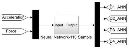
Figure 5 NN Simulink implementation (delay regulation).

Table 2 NN topology parameters

Parameter	Data
Inputs	F and dv
1st hidden layer neurons	10
Outputs	D1, D2, D3 and D4
Number of epochs	27
Regression	0.8, the closer R is to one, the stronger the model.
Number of training data	110 samples.
Training method	Levenberg–Marquardt BP.
Activation function type	Tangent sigmoid (tansig), while linear activation functions (purelin) are employed at the output layers.
Validation checks	6 (early stopping), the maximum number of consecutive iterations that the validation performance fails to decrease. If it reaches, the training will end to stop overfitting.
Mean squared error (mse)	3.7e.⁻⁵ at epoch 21, the closer mse to zero, the more accurate model.

(II) Training Data Generation

The GA calculates the optimum delay time by minimizing the CRMS error based on Equation (4) in different scenarios.

C R M S = {(\frac{1}{T} \int_{t =0}^{T} {‖ u (t) ‖}^{2} d t)}^{1/2}

(4)

where the CRMS error is the cumulative root mean square error and u(t) is the variation between the output speed and the reference signal.

In this study, GA is chosen because it can be employed for a wide variety of problems, has a higher chance of reaching a global optimum solution than traditional optimization methods, and the search space is not well understood (Sivanandam and Deepa, 2008).

Table 3 Specifications of the GA model

Parameter	Data
Reference variable	Speed at specific accelerations and specific loads.
Correcting variables	D1, D2, D3 and D4 together at every iteration.
Optimization stopping criteria	The optimization iteration is restarted when the maximum speed is reached.
Objective	Minimize the CRMS error.

No specific rule was found for the optimal number of samples required for the NN, but in general, large quantities of input/output data and few hidden neurons yield the best results. A simple method of determining the quantity of required training data is to apply the following minimum and maximum thresholds for training samples (Lawrence and Petterson, 1993),

M i n n u m b e r =2 \times (i n p u t s + h i d d e n n e u r o n s + o u t p u t s)

(5)

M a x n u m b e r =10 \times (i n p u t s + h i d d e n n e u r o n s + o u t p u t s)

(6)

Based on the above limits, between 32 and 160 values should be used. The samples were associated with desired accelerations of 5, 10, 15, 20, 25, 30, 35, 40, 45, and 50 cm/s² and discrete loads of 0, 100, 200, 300, 400, 500, 600, 700, 800, 900, 1000 N; thus, 110 samples were used in total. These samples cover the complete system operating range to develop an accurate model for the NN.

The GA optimized delays are presented in Figure 6. Notably, the four graphs were generated by GA concurrently at every iteration, because the relationship between each dependent variable (output) is not limited to the independent variables (inputs) separately, but also the interactions among the dependent variables themselves, based on the working principle of PCM-coding.

Overall, the developed DFCU (n = 5) (Figure 1) controller (Figure 7) features are as follows.

Pressure-compensated flow is achieved.
The induced delays are predicted.
The valves are distributed based on a binary method with a 0.5 L/min step.
System dynamics and nonlinearities, such as fluid inertia, bulk modulus, supply pressure, and electric motor properties, are considered.
Finally, the inherent response and switching time of each valve are included in the system model. However, the 4/3 valve dynamics and hydraulic resistance were neglected to focus on DFCU performance.

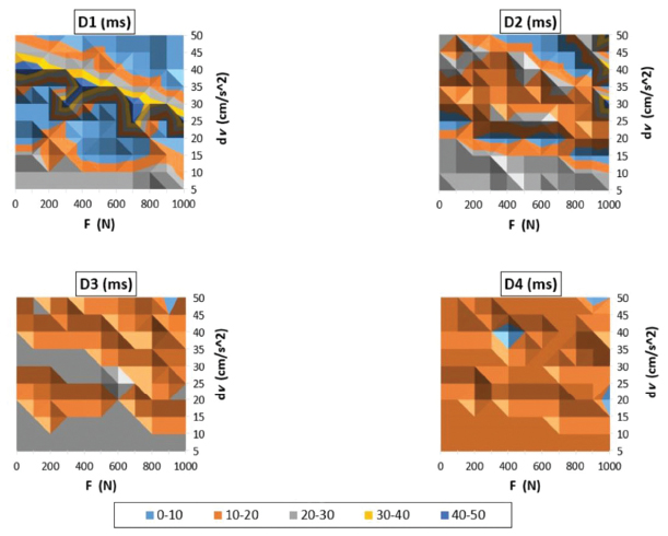
Figure 6 Four contours of the 110 delay samples optimized by the GA for V1, V2, V3 and V4 at different loads and accelerations.

4 Simulation Results

4.1 Controller Delay Testing

4.1.1 Sinusoidal test at maximum load

The results of a sinusoidal input of 1 rad/s at the maximum load, i.e., 1000 N, without the artificial delay NN are presented in Figure 8 (CRMS = 1.8), and the results with a functional NN (CRMS = 1.3) are shown in Figure 9. It is evident that the CRMS is reduced by 28% by applying the NN.

The corresponding separate flow rates are presented in Figure 10. It is clear that the valve overlap is decreased.

A detailed explanation for the poor performance shown in Figure 8 is given in Figure 11. Mainly, a recurrent delay caused by the valve switching regulator. To a lesser extent, the system inertia and the inherent delay of the valve. Notably, V5 should have been operated at 15 Hz to track this trajectory smoothly, while larger valves at relatively lower frequencies.

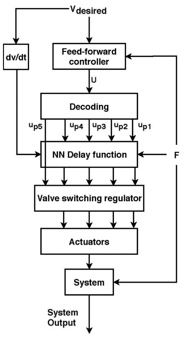
Figure 7 Developed DFCU (n = 5) controller block diagram.

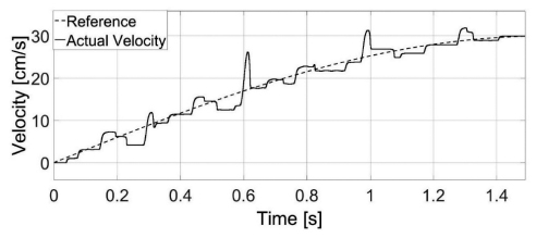
Figure 8 Developed DFCU (n = 5). Sine input reference and the response output at 1000 N (NN is OFF).

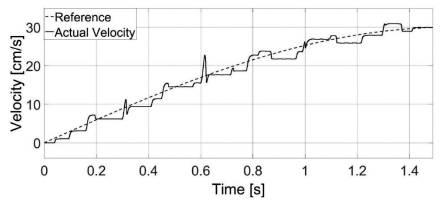
Figure 9 Developed DFCU (n = 5). Sine input reference and the response output at 1000 N (NN is ON).

Figure 10 Valve overlap minimization with the NN for a sinusoidal signal at the maximum load.

The improvement in the tracking accuracy shown in Figure 9 is based on two synchronized stages (Figure 12). (I) NN generates the corresponding delay values at 1000 N load and [30, 2.5] cm/s² acceleration. (II) These values become accessible to the controller at the exact times defined by the delay scheme, previously depicted in Figure 3.

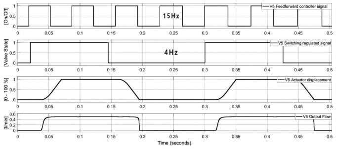
Figure 11 Valve 5 controller signal and the corresponding dynamics, a closer analysis for Figure 8 [0, 0.5] sec.

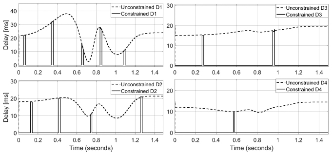
Figure 12 Unconstrained and constrained delay values by the NN architecture (F: 1000 N, dv: 30–2.5 cm/s²) for Figure 9.

The following Table 4 compares the actual delays applied, to the recommended induced delays for an ideal ascending order reference. Because of the relatively steep sine wave and the slow valves, some states were not possible to achieve; consequently, these states were overpassed by the controller. Also, there is no need to delay V5 in this scenario.

Table 4 Performance analysis for the delay scheme applied to DFCU (n = 5)

Parameter	DFCU (n = 5)
Theoretically delayed valves	V1	V2	V1	V3	V1	V2	V1	V4	V1	V2	V1	V3	V1	V2	V1
Actual delayed valves	V1	V2	0	V3	V1	V2	0	V4	V1	V2	V1	V3	V1	V2	0

Flow rate	1	2	3	4	5	6	7	8	9	10	11	12	13	14	15

4.1.2 Sinusoidal test at no load

The results for a sinusoidal input of 1 rad/s at no load and without the NN are presented in Figure 13 (CRMS = 2.4). When the NN is applied (CRMS = 1.5), as shown in Figure 14, the controller performance increases by 38%.

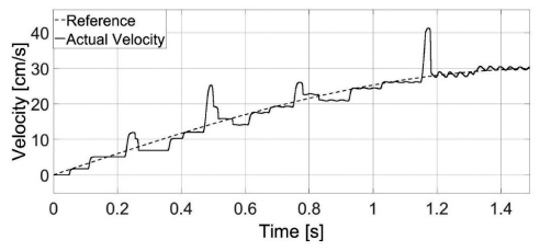
Figure 13 Developed DFCU (n = 5). Sine input reference and the response output at no load (NN is OFF).

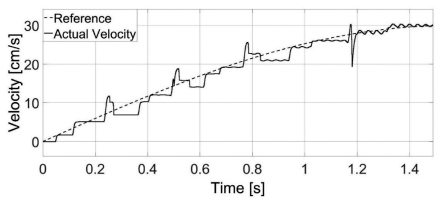
Figure 14 Developed DFCU (n = 5). Sine input reference and the response output at no load (NN is ON).

4.1.3 Variable-load test

In these tests, the fluid inertia was neglected to simplify the simulation, and the corresponding impact on the results was marginal for the defined purpose of this study. The system was tested based on a trapezoidal load (1000 N), as presented in Figure 15. The undershoots and overshoots were caused by rapid, unexpected loads.

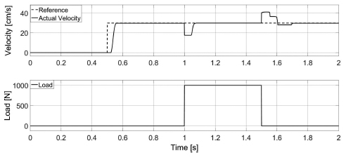
Figure 15 Developed DFCU (n = 5). Trapezoidal load (F) of 1000 N [1, 1.5] sec and the response output.

A ramped input with a high-slope load (dF/dt = 100) is shown in Figure 16. The speed stabilizes after the load settles at 1000 N.

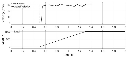
Figure 16 Developed DFCU (n = 5). Ramped load of 1000 N and the response output.

4.1.4 Descending & ascending unordered trajectory tests

The main purpose of this test is to evaluate the delay scheme and further inspect the controller stability.

(A) Descending Unordered

A step input (33 to 21 to 12) cm/s, is presented in Figure 17 (NN is off), and Figure 18 (NN is on). The velocity ripples are due to the system inertia and the absence of a damping factor such as the load.

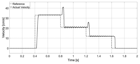
Figure 17 Developed DFCU (n = 5). Descending unordered reference and the response output at No load (NN is OFF).

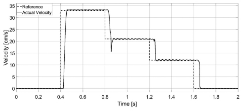
Figure 18 Developed DFCU (n = 5). Descending unordered reference and the response output at No load (NN is ON).

The corresponding valves for this trajectory are (I: V1, V5, V4 to II: V3, V2 to III: V2, V1, V5), and as previously explained, the valves that should be delayed are I: None. II: Both V2 and V3. III: V1 and V5 only, as shown in Figure 19.

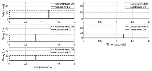
Figure 19 Unconstrained and constrained delay values by the NN architecture for descending unordered trajectory (F: no load, dv: constant).

(B) Ascending Unordered

A step input (12 to 21 to 33) cm/s, is presented in Figure 20 (NN is off), and Figure 21 (NN is on).

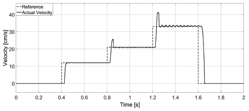
Figure 20 Developed DFCU (n = 5). Ascending unordered reference and the response output at No load (NN is OFF).

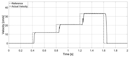
Figure 21 Developed DFCU (n = 5). Ascending unordered reference and the response output at No load (NN is ON).

The corresponding valves for this trajectory are the same as in the previous test, but in reverse order, i.e., (I: V2, V1, V5 to II: V3, V2 to III: V1, V5, V4). However, the valves that should be delayed are I: None. II: V3. III: V1, V5 and V4, as shown in Figure 22.

Discussion

Interestingly, V5 required to be delayed in both tests. The delay state-oriented technique shown in Figure 3 can easily determine the exact time suitable for implementing the delay values for V5. However, determining the value of this delay, i.e., D5, wasn’t either optimized using the GA nor predicted using the NN, while a constant predetermined value of 15 ms was given to the controller, for the following reasons:

(I) V5, which is the smallest valve, has a minimal effect on the pressure peaks in the system.

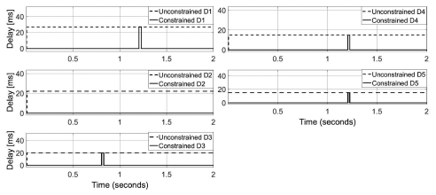
Figure 22 Unconstrained and constrained delay values by the NN architecture for ascending unordered trajectory (F: no load, dv: constant).

(II) The conditions at which V5 should be delayed are relatively limited, particularly in ascending transition states. In a DFCU (n = 5), the number of every possible “paired” states is 2ⁿ P “2” = 992. While the number of ascending, unordered transition states in which V5 needs to be delayed is 55, as shown in Table 5. In descending transition states, V5 should be delayed whenever it opened, i.e., 1/2 × 2ⁿ⁻¹ P 2 = 120, this is because the number of states in which the smallest valve is ON in the “descending” order is “1/2” × 2ⁿ⁻¹.

Table 5 Delay times required for the V5 in DFCU (n = 5), during ascending, unordered transition states at the ideal operating conditions (V1: 1Q, V2: 2Q, V3: 4Q, V4: 8Q, V5: 0.5Q)

From Total Flow Rate (Q)	To Total Flow Rates (Q)
1	2.5, 4.5, 6.5, 8.5, 10.5, 12.5, and 14.5.
2	4.5, 5.5, 8.5, 9.5, 12.5, and 13.5.
3	4.5, 5.5, 6.5, 8.5, 9.5, 10.5, 12.5, 13.5, and 14.5.
4	8.5, 9.5, 10.5, and 11.5.
5	6.5, 8.5, 9.5, 10.5, 11.5, 12.5, and 14.5.
6	8.5, 9.5, 10.5, 11.5, 12.5, and 13.5.
7	8.5, 9.5, 10.5, 11.5, 12.5, 13.5, and 14.5.
9	10.5, 12.5, and 14.5.
10	12.5, and 13.5.
11	12.5, 13.5, and 14.5.
13	14.5.

(III) To optimize the delay values of the smallest valve, D5, an additional laborious optimization process could be done by either one of these two proposals. (A) Rerunning the GA model at negative speed slopes (descending order), i.e., dv = negative. (B) Creating scenarios simulating the 55 ascending, unordered transition states, to be subsequently run by the GA. Finally, feed these optimized samples to the NN. These suggested solutions are left for future studies to explore.

5 Conclusion

A controller is proposed for a digital hydraulic system coded with PCM. The use of an NN yielded a considerable reduction in the tracking error of up to 38%. The feedforward controller is better suited than the traditional feedback controller for regulating artificial delays. Notably, because of the rapid occurrence of pressure peaks, i.e., rapid surges and declines, once the valve receives the ON command, the feedback controller cannot respond and reduce the resulting error.

These findings could be extended and applied in separate meter-in and meter-out circuits. Referring to the earlier studies of DVS control and due to the previously discussed problems with PCM; many researchers have implemented PNM control methods. Therefore, with the aid of the proposed delay controller, PCM has extensive application potential in the flow control field.

However, the system still has some issues, such as those associated with fast demand acceleration or sudden loads, which are related to the slow valve response. Another important point to consider is that typical DFCUs operate at higher frequencies than 4 Hz, still, with the aid of the proposed controller and the same employed principle, pressure peaks could be studied for minimization. It should be noted that fast valves are also characterized by inherent problems, such as noise, severe hammering effects, and high costs. Another point to consider, the delay value of the smallest valve in the system, i.e., valve 5, wasn’t optimized using the GA, while this value was tuned aiming to mitigate the pressure peaks in specific scenario, which is not necessarily the optimum value in different conditions.

Finally, the paper managed to minimize the pressure peaks in a PCM metering hydraulic circuit using NN and hence increases the tracking accuracy.

Nomenclature

Quantity	Description	Unity
A_A	Piston area (piston side)	m²
A_B	Piston ring area (rod side)	m²
A_o	Orifice area	m²
A_v	Valve effective cross-sectional area	m²
CRMS	Cumulative root mean square error	–
C_d	Coefficient of discharge	–
Di	Delay inputs for valves, i = 1...5	ms
F	Force/Load	N
F_r	Rated load	N
n	Numbers of valves	valve
P_B	Pressure in chamber B	Pa
P_cr	Minimum pressure for turbulent flow	Pa
P_s	Supply pressure	Pa
Q	Flow rate	m³/s
Q_N,Pi	Nominal flow of the i-th pump side valve, i = 1...5	(m³/s) Pa^1/2
T	Periodic time	s
u_p	State of the pump side digital flow control unit	–
u_pi	Control signal of the i-th pump side valve	–
V	Valve	–
v_desired	Piston desired velocity	cm/s
v_r	Rated load velocity	cm/s
ΔP_o	Orifice differential pressure	Pa
ΔP_v	Valve rated pressure	Pa
ρ	Fluid density	kg/m³
ω_n	System natural frequency	Hz

Acronyms

Acronym	Description
BP	Backpropagation
DFCU	Digital flow control unit
GA	Genetic algorithm
MLFNN	Multi-layered feedforward neural network
NN	Neural network
PCM	Pulse code modulation
PNM	Pulse number modulation

References

Dong, G., Fataliyev, K. and Wang, L. One-step and multi-step ahead stock prediction using backpropagation neural networks. 2013 9th International Conference on Information, Communications & Signal Processing, 2013. IEEE, 1–5.

Elsaed, E., Abdelaziz, M. and Mahmoud, N. A. 2017. Investigation of a digital valve system efficiency for metering-in speed control using MATLAB/Simulink. International conference on hydraulics and pneumatics-23rd edition (HERVEX) 2017 Băile Govora, Romania. HERVEX, 120–129.

Huova, M., Linjama, M. and Huhtala, K. 2013. Energy efficiency of digital hydraulic valve control systems. Commercial vehicle engineering congress 2013 Illinois, USA. SAE International.

Hydraulics, S. 2018a. DTDBXCN212N [Online]. Available: http://www.sunhydraulics.com/model/DTDB/XCN212N [Accessed 2018].

Hydraulics, S. 2018b. FPCCXAN214N Electro-proportional flow control valve – normally closed [Online]. Available: http://www.sunhydra ulics.com/model/FPCC/XAN214N [Accessed 2018].

Jelali, M. and Kroll, A. 2012. Hydraulic servo-systems: modelling, identification and control, Springer Science and Business Media, 220–221.

Ketonen, M., Huova, M., Heikkilä, M., Linjama, M., Boström, P. and Walden, M. 2012. Digital hydraulic pressure relief function. Fluid power and motion control (FPMC), 2012 University of Bath, UK. Center of power and motion control, University of Bath, ASME, 137–150.

Laamanen, A., Linjama, M. and Vilenius, M. 2003. Characteristics of a digital flow control unit with PCM control. 7th Triennial international symposium on fluid control, measurement and visualization, 2003 Sorrento, Italy. Optimage Ltd., Edinburgh, UK, EH10 5PJ, 1–16.

Laamanen, A., Linjama, M. and Vilenius, M. 2005. Pressure peak phenomenon in digital hydraulic systems – a theoretical study. Power transmission and motion control (PTMC), 2005 University of Bath. John wiley and sons, 91–104.

Laamanen, A., Linjama, M. and Vilenius, M. 2007. On the pressure peak minimization in digital hydraulics. The tenth scandinavian international conference on fluid power (SICFP’07), 2007 Tampere, Finland. Tampere University Technology.

Laamanen, A., Siivonen, L., Linjama, M. and Vilenius, M. 2004. Digital flow control unit – an alternative for a proportional valve? Bath workshop on power transmission and motion control, 2004 University of Bath, UK. Professional engineering publishing, 297–308.

Laehteenmaeki, T., Ijas, M. and Mäkinen, E. 2010. Characteristics of digital hydraulic pressure reducing valve. Fluid power and motion control (FPMC), 2010 University of Bath, UK. Center of power and motion control, University of Bath, ASME, 69–82.

Lawrence, M. and Petterson, A. 1993. Brainmaker Professional: neural network simulation software user’s guide and reference manual, California scientific software.

Linjama, M., Huova, M., Karhu, O. and Huhtala, K. 2016. High performance digital hydraulic tracking control of a mobile boom mockup. 10th international fluid power conference, 2016 Dresden, Germany. Technical University Dresden.

Linjama, M., Koskinen, K. T. and Vilenius, M. 2002a. Pseudo-proportional position control of water hydraulic cylinder using on/off valves. International symposium on fluid power (JFPS), Japan. The japan fluid power system society, 155–160.

Linjama, M., Koskinen, K. T. and Vilenius, M. 2003. Accurate trajectory tracking control of water hydraulic cylinder with non-ideal on/off valves. International Journal of Fluid Power, 4, 7–16.

Linjama, M., Sairiala, H., Koskinen, K. T. and Vilenius, M. 2002b. Highspeed on/off position control of a low-pressure water hydraulic cylinder drive. 49th National conference on fluid power, Las Vegas, USA. SAE International, 217–225.

Linjama, M. and Vilenius, M. 2004. Digital hydraulic control of a mobile machine joint actuator mockup. Bath workshop on power transmission and motion control, 2004. Professional Engineering Publishing, 145–158.

Linjama, M. and Vilenius, M. 2007. Digital hydraulics – Towards perfect valve technology. The tenth scandinavian international conference on fluid power (SICFP’07), 2007 Tampere, Finland. Tampere University Technology.

Mathworks. 2006. Hydraulic orifice with constant cross-sectional area [Online]. [Accessed 2018].

Mirzaee, H. 2009. Long-term prediction of chaotic time series with multi-step prediction horizons by a neural network with Levenberg–Marquardt learning algorithm. Chaos, Solitons and Fractals, 41, 1975–1979.

Morel, L. and Boström, P. 2007. Design and Implementation of energy saving digital hydraulic control system. The tenth scandinavian international conference on fluid power (SICFP), 2007 Tampere, Finland. Tampere University Technology, 341–359.

Nelles, O. 2013. Nonlinear system identification: from classical approaches to neural networks and fuzzy models, Springer Science and Business Media, 252.

Ottenbacher, K. J., Linn, R. T., Smith, P. M., Illig, S. B., Mancuso, M. and Granger, C. V. 2004. Comparison of logistic regression and neural network analysis applied to predicting living setting after hip fracture. Annals of Epidemiology, 14, 551–559.

Sivanandam, S. and Deepa, S. 2008. Genetic algorithms. Introduction to genetic algorithms. Springer.

Svozil, D., Kvasnicka, V. and Pospichal, J. 1997. Introduction to multilayer feed-forward neural networks. Chemometrics and intelligent laboratory systems, 39, 43–62.

Yu, H. and Wilamowski, B. M. 2011. Levenberg-marquardt training. Industrial electronics handbook, 5, 15.