Fast Modelling and Identification of Hydraulic Brake Plants for Automotive Applications
Luca Pugi1,*, Federico Alfatti1, Lorenzo Berzi1, Tommaso Favilli1, Marco Pierini1, Bart Forrier2, Thomas D’hondt2 and Mathieu Sarrazin2
1Università degli Studi di Firenze, Dipartimento di Ingegneria Industriale, Italy
2Siemens Industry Software NV, Belgium
E-mail: luca.pugi@unifi.it
*Corresponding Author
Received 16 June 2020; Accepted 21 September 2020; Publication 27 November 2020
Abstract
Diffusion of electric and hybrid vehicles is accelerating the development of innovative braking technologies. Calibration of accurate models of a hydraulic brake plant involves availability of large amount of data whose acquisition is expensive and time consuming. Also, for some applications, such as vehicle simulators and hardware in the loop test rig, a real-time implementation is required. To avoid excessive computational loads, usage of simplified parametric models is almost mandatory. In this work, authors propose a simplified functional approach to identify and simulate the response of a generic hydraulic plant with a limited number of experimental tests. To reproduce complex nonlinear behaviours that are difficult to be reproduced with simplified models, piecewise transfer functions with scheduled poles are proposed. This innovative solution has been successfully applied for the identification of the brake plant of an existing vehicle, a Siemens prototype of instrumented vehicle called SimRod, demonstrating the feasibility of proposed method.
Keywords: Identification, modelling, brake plants, piecewise transfer function, linear systems with scheduled poles.
1 Introduction
There is a wide literature [1–5] concerning simulation of conventional automotive brake plants, which is usually performed using customized commercial tools.
These models are used to reproduce the behaviour of complex pneumatic-logic [6–8] or hydro-mechanics systems, according to chosen application.
Different innovation trends of automotive sector are boosting the proliferation of different brake plant configurations.
Development of electric powertrains [9, 10] and pervading diffusion of autonomous or assisted driving systems [11–13] are encouraging the application of brake-by-wire technologies [14].
More generally, there is an increasing interest for studies concerning innovative brake plant configurations [15–18] to improve both performances and implemented functionalities.
As example, Zhao et al. [17] proposed to perform an easy and robust management of both conventional and regenerative braking.
Same topics are also discussed by Ma et al. [19], whose work is more focused on the development of an electric braking unit.
Finally, in his work, Zhang [20] investigates how to optimize actions of conventional and regenerative braking systems.
These works emphasize different aspects of a common topic: the need of an increasing integration between a conventional brake system, electric powertrain and various vehicle systems through VCU (Vehicle Control Unit).
As a part of OBELICS project (Optimization of scalable rEaltime modeLs and functIonal testing for e-drive ConceptS), authors have to develop general purpose models that should be used to reproduce and fit the functionalities of different braking plants that are installed on a wide variety of vehicles:
• Light Vehicle (with various kind of powertrain);
• Car of A,B,C segment (ranging from Citycar to a Compact one);
• Truck;
• Sport Vehicle (mainly designed for recreational activities).
In this sense, the work is not only a relevant result of the overcited research project but also an original research contribution respect to exigences of major automotive industrial players that have sustained not only this specific project but also the whole European research call H2020 in which these topics are widely addressed.
Looking at the list of different kind of vehicles, it is difficult to obtain a pure physical model that fit the behaviour of different brake plants by accurately modelling each sub-component. Also a certain level of abstraction of the model should be very important in order to assure the portability of proposed models between different simulation environments like Siemens-Simcenter or Matlab-Simulink.
As example, in literature there are specific works dedicated to the modelling of ABS controllers and hydraulic brake plants [21].
Also, in literature, it is easy to find brake models which are optimized for a specific vehicle or plant layout.
However, there is a gap for what concern simplified general models that can be used to fit plant functionality abstracting from specific physical features of components and subsystems.
Also, very accurate models involve the availability of a large amount of data and the calibration of many parameters, which are often not available.
For these reasons, a general-purpose procedure is proposed and investigated in this work.
Proposed approach should be usable for different tasks and activities:
• Preliminary Design, Simulations and Numerical Optimizations.
• Real-Time Implementation for Hardware-in-the-Loop (HiL), Software-In-the-Loop (SiL) and Model-in-the-Loop (MiL) systems.
• Re-use of proposed models as part of model-based filters, controllers and estimators.
In this work it is proposed a hybrid functional model: simple physical elements are introduced to perform an easy calibration; more complex functionalities are implemented with interpolated piece-wise linear transfer functions, able to fit a wide variability of different behaviours acting on a reduced set of parameters.
Usage of interpolated piece-wise linear transfer functions is an innovative contribution that authors have developed and applied from previous railway applications: in previous activities authors have modelled complex response of pneumatic elements of the Direct Electropneumatic Brake (UIC) [22] and their interactions with more advanced control functionalities such as brake blending [23] or Wheel Slide Protection (WSP) system.
Piece-wise linear transfer functions are a powerful instrument that is commonly used to approximate systems with a strong nonlinear behaviour, minimizing the number of integrated states and maintaining a high level of continuity on calculated states and corresponding derivatives.
Piece-wise linear transfer functions are widely proposed and adopted in literature [24] to perform robust model reduction of systems with non-linear or badly scaled dynamics [25, 26].
Authors have considered an existing electric sport vehicle the Kyburz E-rod as benchmark test vehicle.
Kyburz E-rod has been modified by Siemens laboratories, in Leuven, to produce a prototype of a special Electric Vehicle (EV), called SimRod.
This vehicle has been provided by Siemens, one of the partners of OBELICS project.
Siemens has also managed a large part of experimental activities, including sensors and logistic support.
Original contributions of this research respect to current literature are mainly two:
• Functional Decomposition of the Plant: proposed model it is not a simplified physical representation of the plant, but of its functionalities. Simplified physical sub-models are introduced only to make possible an easy tuning of proposed model respect to experimental data.
• Piece-wise Transfer Functions: poles of linear transfer functions are scheduled respect to state values and their derivatives. In this way it is possible to reproduce complex nonlinear phenomena affecting both amplitude and frequency response of the plant. Resulting model maintains a low number of integrated states and assures a numerically smooth behaviour.
In this way, authors were able to verify flexibility and fitting capabilities of the proposed modelling approach.
Paper is organized as follow:
• in Section 1 authors introduce a brief general description of proposed brake model including sketches, equations and corresponding functionalities.
• In Section 2 it is described the application of the proposed model to the chosen benchmark vehicle, Siemens Simrod.
• Vehicle and sensor layout used for experimental activities are described in Section 3.
• Results of performed identification procedures are discussed in Section 4 showing the simplicity and the general applicability of proposed method.
• In Section 5 further experimental data are compared with simulation results to validate the model respect to various braking pattern recorded on the vehicle when tested on the the circuit of Aldenhoven (Germany).
2 Brake System Model
Authors started their work from a general scheme of a brake plant taken from literature [27], which is visible in Figure 1.
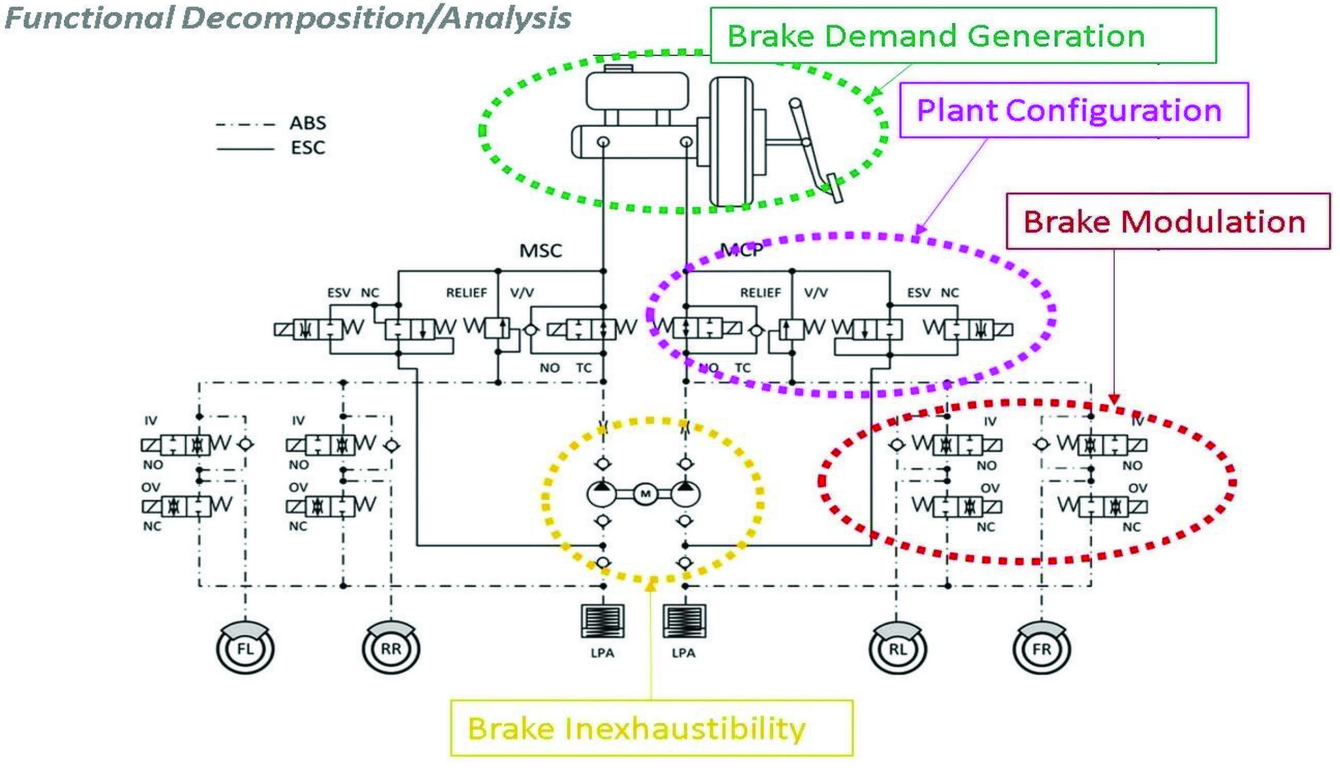
Figure 1 Simplified functional scheme of generic brake plant [27].
Brake Plant is analysed in terms of implemented features and functionalities to better understand how to generalize and simplify proposed simulation model:
• Brake Demand Generation: desired brake demand is generated by a human driver or by automatic/autonomous systems that assist or substitute his action. In this work it is considered as a signal that have to be servo-amplified and eventually filtered, to obtain desired plant response.In electric vehicles, application of braking forces is often redundant, due to the contemporaneous presence of electric and conventional brakes. So, systems devoted to generation of brake demand has also to properly decide an optimal allocation-blending strategy.
• Brake Modulation: each wheel is actuated by an independent hydraulic unit. Hydraulic control unit is supposed to be controlled by regulating its inlet and outlet flow.
• Plant Configuration: several systems have to control and modulated braking forces exerted on each wheel, modifying the brake demand reference. Typical examples are represented by Anti-lock Braking System (ABS), Electronic Stability Program (ESP) system or more generally by any subsystem which must modulate longitudinal forces on wheels to assure higher level of stability and safety performances. In a real plant this modulation is performed by many valves, which are also needed to produce a specific variation of the plant topology.
• Inexhaustible Braking: action of brake plant and its interactions with on-board systems such as ABS or ESP should produce an increased demand of hydraulic power. Brake plant must be able to supply enough hydraulic power to assure a proper braking also in these situations.
To fit the functional behaviour of a generic brake plant, authors propose a simplified pseudo-physical model, whose main features are briefly described in Figure 2.
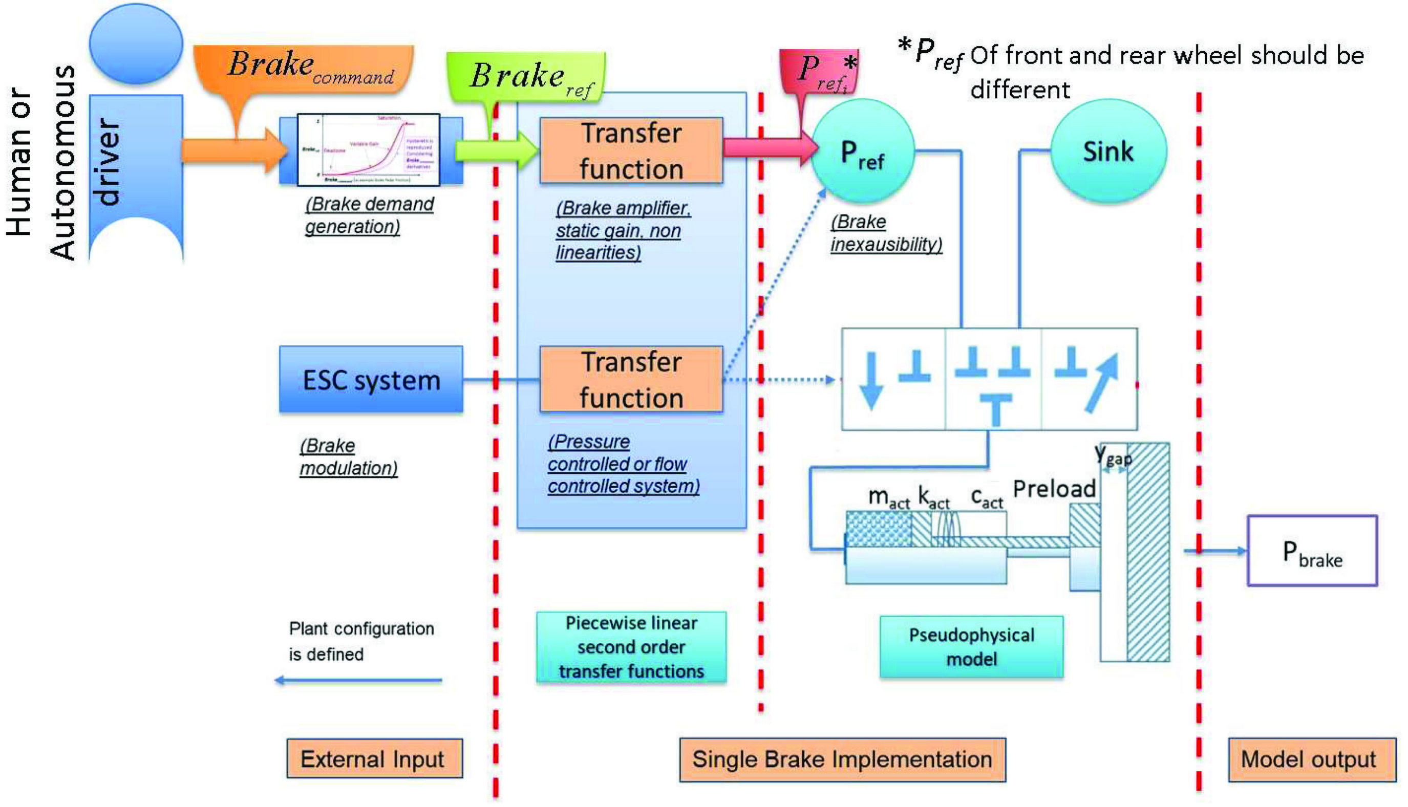
Figure 2 Simplified pseudo-physical model proposed by university of Florence.
Brake Demand is pre-processed using a piece-wise second order transfer functions.
Static gain of the transfer function is scheduled to fit plant response in terms of amplitude.
Poles of the transfer function are scheduled respect to system states, to reproduce dynamic response of brake plant including non-linear features.
Output of this transfer function is an equivalent pressure reference, corresponding to the desired torque that must be transmitted to braking units.
This reference pressure is modulated considering an independent actuation unit for each wheel. In this way it is possible to control the brake force applied on each wheel by controlling the clamping force applied by each calliper.
To model the simplified hydraulic plant of callipers, a multi-physics approach [28] is followed. Fluid compressibility is modelled as a single R-C (resistive-capacitive elements) that simulate equivalent capacity and losses of the plant.
This hydraulic model is coupled with a lumped mechanical model with a Single Degree Of Freedom (DOF) able to simulate mechanical response of the calliper.
Many on board subsystems have to modulate brake forces on wheels, such as example, ABS and ESP.
In order to control the brake force of each wheel, actuation of each calliper is controlled by another valve which is also modelled using piecewise second order transfer function.
Inexhaustible Braking behaviour is current implemented supposing a proper design of the system, so pressure reference P is modelled as an ideal pressure source.
However, limitations of a real pumping unit can be easily simulated by considering a real pressure source, whose response is limited by a fixed or a scheduled hydraulic loss coefficient.
Proposed UNIFI brake model has been developed in order to be implemented on most commonly tools and simulation platforms devoted to the simulation of automotive systems, like Matlab Simulink and Siemens Simcenter.
2.1 Brake Demand Generation
Brake demand is assumed to be generated by a human or an autonomous driver as a dimensionless reference Brake (ranging from 0 to 1).
Brake represents the required braking performance generated by an input signal called Brake. An example of Brake is the run of brake pedal which is used by the human driver to activate vehicle brake.
Brake is a tabulated function of the input Brake and its derivative, as visible in Figure 3. In this way it is possible to reproduce some non-linear behaviour of system response, such as dead-zones, variable gains, saturation effects, etc.

Figure 3 Example of feed-forward tabulation for Brake respect to Brake.
Longitudinal braking torques have to be distributed among rear (T) and front wheels (T ) according to optimal allocation criteria, commonly adopted in literature [29]. Efforts are allocated according to (1) and (2) by and Electronic Braking Distribution (EBD) controller.
| (1) | ||
| (2) |
Where
i= f, r respectively for front and rear wheels,
K adopted in (1) are scaling factors which differ between front (K) and rear(K) wheels whose values assure the proper scaling of braking forces described in (2)
a is the longitudinal distance between front axle and the vehicle center of gravity and
b the longitudinal distance between the latter and the rear axle.
h is the height of the center of mass of the vehicle respect to ground
g is defined as gravity acceleration (about 9.81 ms)
Once desired longitudinal forces T and T are known, corresponding values of steady state pressure P, called P, can be calculated according to (3).
| (3) |
The following symbology is adopted:
• A is the equivalent area of the calliper (including friction surfaces and actuators);
• F, k and y are respectively the pre-load, stiffness and run of the calliper;
• r and are the mean disc radius and the mean rolling radius of the wheel.
• f is the friction factor between brake pads and discs.
• P is the steady state value of brake pressure P that should be applied to the brake calliper in order to obtain the desired value of longitudinal brake force T, in steady state conditions.
Pressure reference P is generated by a servo-amplified power source that has a dynamical behaviour with a finite bandwidth.
Assuming to model the system as an equivalent pressure-controlled loop, transfer function described in (4) is used to represent evolution of P respect to the desired steady state value P:
| (4) |
Where in (4), following symbology is adopted:
is the equivalent eigenfrequency/pole of the pressure loop (ranging from 10 to 10 Hertz according system performances )
is the damping factor (typically ranging from 0.7 to 1)
Second Order transfer functions are often used to approximate the dynamical behaviour of both flow-controlled and pressure-controlled valves: this approach was initially proposed by historic manufacturer of valves like Moog [30] and it’s also recognizable in classic handbook like Merrit [31] and it is currently adopted by simulation software such as AMESIM Simcenter Finally also in recent research works [32], transfer functions (second order or superior) are still commonly used to represent the behaviour of hydraulic valves.
Transfer Function (4) is often a rough approximation of plant response, so authors adopted a piece-wise linear transfer function in which parameters and are scheduled as functions of system states.
Variable coefficient transfer functions are not usually available in common simulation environments, so authors implemented the transfer function described in (4) according the scheme of Figure 4. Integration scheme of Figure 4 it is implemented using only simple blocks such as integrators, gains and summing elements that are available almost in every simulation environment.
In this way, it’s possible to change the coefficients of transfer function with continuous smooth behaviour: even a step variation of transfer function coefficients produces an output signal which is at least C1(continuity of function and of its first derivative).
In this way it is possible to properly shape a smooth and continuous behaviour of simulated pressure reference P.
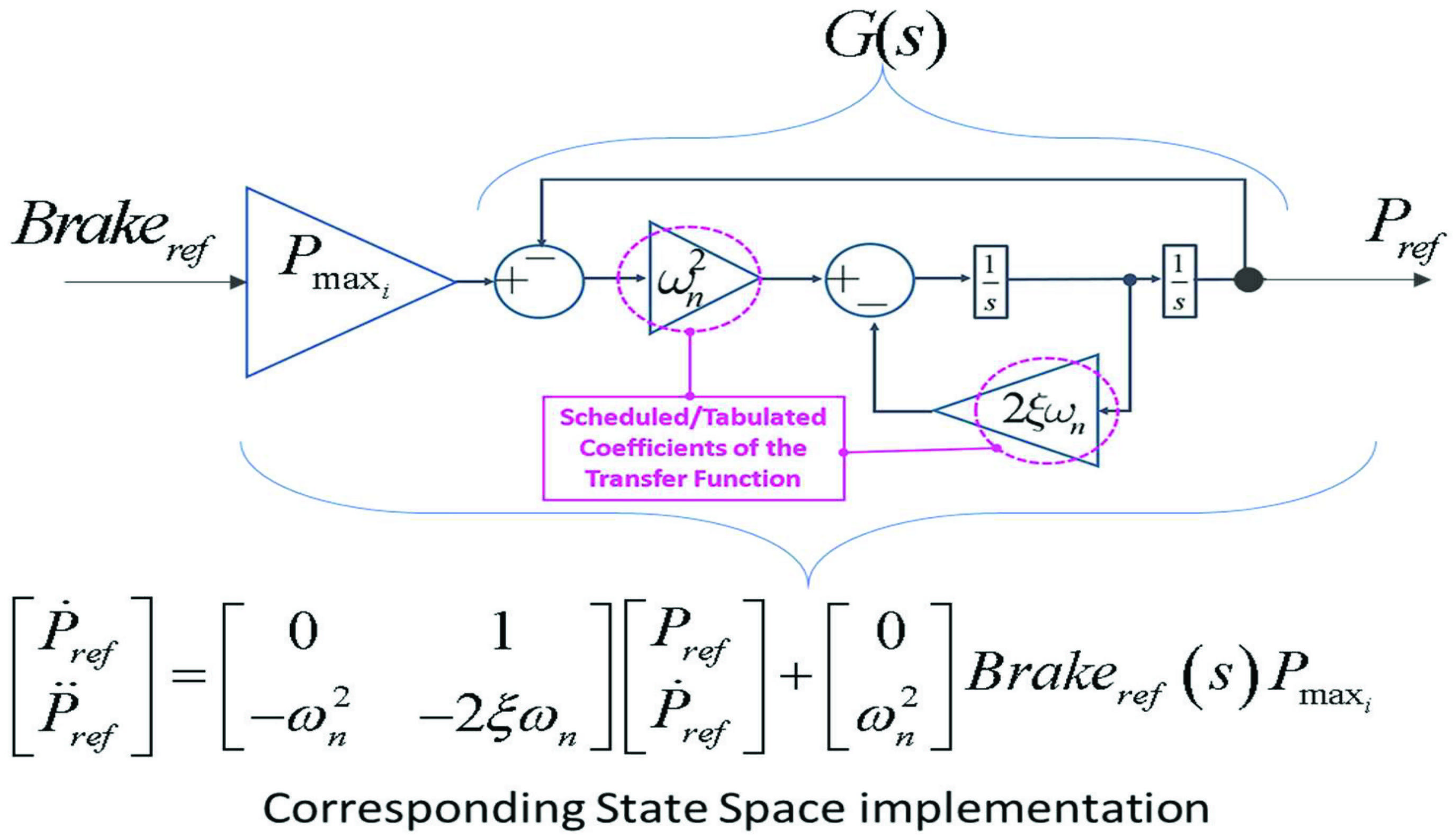
Figure 4 Implementation of equation (4).
2.2 Brake Actuator Model
Pressure reference P, calculated according (4), represents from a physical point of view the output pressure provided by the brake amplifier of the plant which is used to feed brake actuators as described by the scheme of Figure 5: P is modelled as an ideal pressure source which is used to feed the actuator, a single chamber cylinder with preload springs through a three way valve. This three-way valve that is normally open when ABS is not working, introduces pressure drops and consequently flow limitations that are useful to properly fit the response of a real plant.
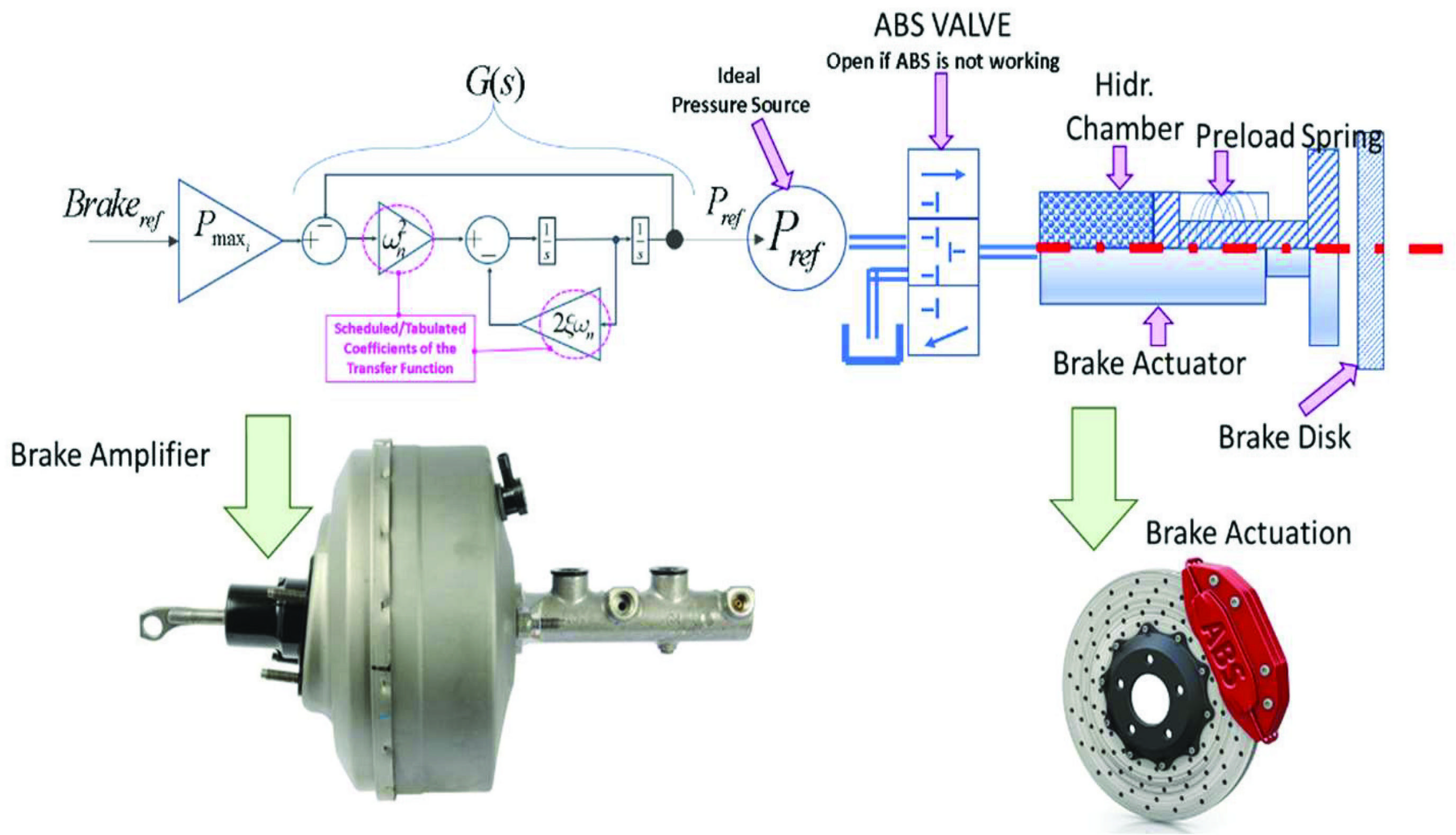
Figure 5 Implementation of a control loop to used impose the pressure of the actuator.
Flow Q that feed brake actuator is computed according (5) which calculates flow through the valve of Figure 5 from known values of P and p (pressure inside the i-th brake cylinder), knowing valve state x and nominal flow Q:
| (5) |
Mass flow rate is calculated according (6) once fluid density is known:
| (6) |
Following symbology is adopted in (5) and (6):
• Q and P are the rated flow and the pressure of the modelled orifice.
• p and are respectively the pressure of the connected chamber of the hydraulic actuator and the inlet fluid density.
• x is a valve state signal, for which a value of 1 indicates a braking action and a value of indicates a fully released brake. Admitting a continuous range of values for x would yield a proportional valve model. A change of the valve command x is used to represent the behaviour of the ABS plant aiming to modulate the clamping pressure of the actuator. If ABS is not working the valve is open () acting as a fixed area orifice which is quite useful to roughly fit hydraulic losses of the plant.
To solve equation (6) cylinder pressure p must be known: so resistive model of the valve orifice must be coupled with a second relationship (7) that calculate p considering fluid compressibility effects in actuator chamber.
| (7) |
In (7) following symbology is adopted: is the temperature expansion coefficient and is the bulk modulus of the fluid.
Assuming an isothermal behaviour and substituting the inverse of the density with the specific volume v, equation (7) can be rewritten as (8)
| (8) |
In (8), following symbology is adopted:
• v and V are respectively specific volume of fluid and volume of actuator chamber.
• m is the mass of brake fluid in the capacitive element of the actuator.
Volume V, according (9), can be expressed as function of the following parameters: displacement y, minimum actuator volume V and piston surface A.
| (9) |
Displacement y is calculated from (10) where is considered dynamical equilibrium due to different forces applied to brake actuator: internal pressure force pA is balanced by inertial forces due to actuator mass m, and by visco-elastic forces due to actuator preload , Stiffness k and viscosity c.
Preload maintains a gap, i.e. a positive clearance y, between pads and disc when the brake is released. If a null clearance is achieved (yy), a contact constraint is considered (run y is saturated to y); then contact force able to maintain equilibrium is calculated: if F is negative, contact is disengaged and the pad is free to leave the disc.
| (10) |
All the over described equations (1–10) have been implemented in a Matlab-Simulink Model with a robust/stiff fixed step solver (Ode 14x). This implementation was preferred to more recent Simulink Toolbox (like Hydraulic blocks of Simulink-Simscape) mainly for two reasons:
• Real Time Implementation: using standard Simulink blocks and a fixed step solver is possible to assure a real-time implementation with modest computational resources (sampling frequency lower than 1kHz, reduced number of integrated states).
• Portability on different environment/software: using a limited number of blocks with very simple functionalities (summing and integrating block) is relatively simple to export or reproduce the same approach also in other simulation environments such as Siemens Simcenter.
A Simplified Scheme with a Snapshot of the model is shown in Figure 6a.
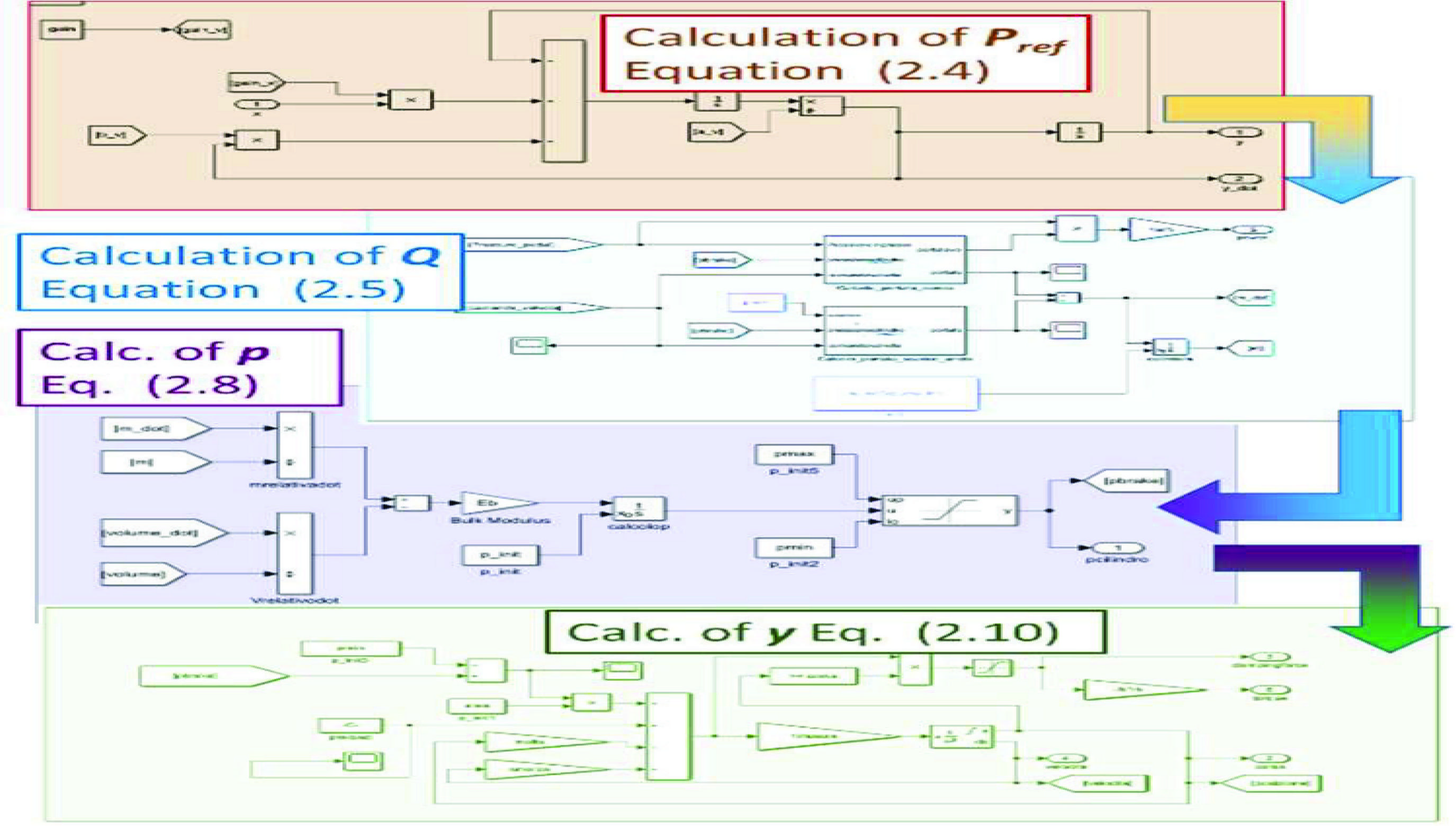
Figure 6a Simulink Model Brake Plant with some snapshots on most significant subsystems.
In Figure 6b is shown an example of simulation in which is reproduced the step application of braking forces followed after one second by a step release of the brake: for front and rear brake cylinders is supposed a different braking pressure (65 and 40 bar respectively):this benchmark model is still not calibrated or tuned for a precise case study since the aim of this example is only to demonstrate some potential feature of the proposed approach;as visible in Figure 6b, application and release of brake effort is delayed by a transient which is mainly influenced by the choice of parameters and (4) that describes plant dynamics. In this example and are constant so plant have the same response time in both braking and release phases. It is interesting to notice the effect of actuator airgap y and of preload F: when brake effort is applied, pressure rises; as pressure is able to win spring preload, actuator starts to move recovering the airgap distance between pad and disc. In this phase cylinder pressure is almost constant since a large flow is needed to move the piston while modest additional forces are needed since the calliper is moving in the air. As the gap is completely recovered, contact between pad and disc is engaged. In this phase pressure starts to rise again reaching the desired steady state value. A similar coherent behaviour is also recognizable during the release phase.
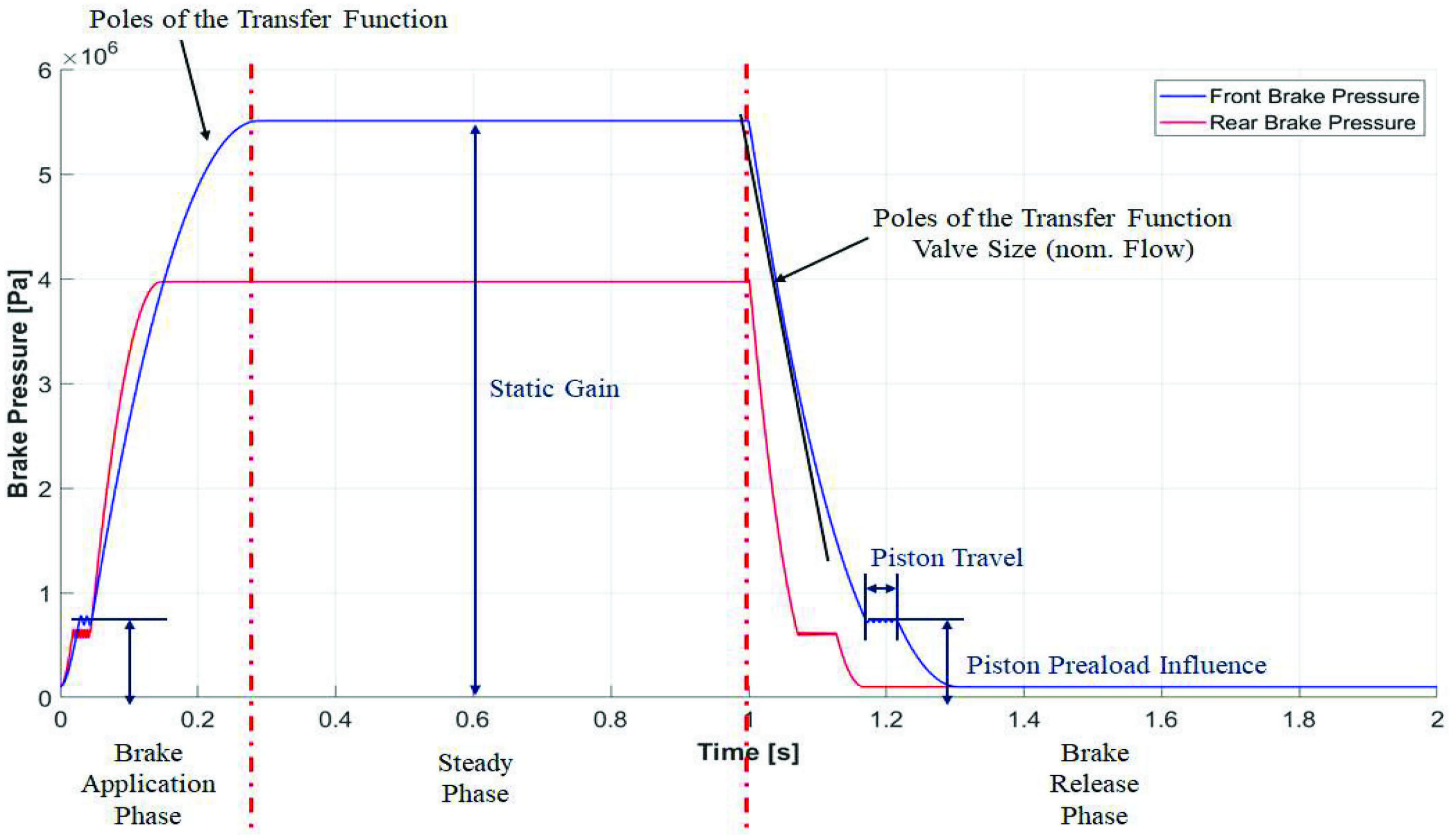
Figure 6b Example fitting capability of the proposed model.
2.3 Brake Actuator Model Plant Configuration: Interfacing with ABS/ESP/ESC Systems
On modern vehicles, brake plant is interconnected with several on board control and safety systems, e.g. ABS [33] or ESP/ESC [34]. These systems may overrule or modulate demanded braking efforts. This functionality is typically assured by a system of fast response valves (visible in the example of Figure 1) which intercepts the fluid flow that is provided for brake clamping: if the force of the i-th brake cylinder has to be modulated, his internal pressure p is regulated by alternatively connecting the cylinder with pressurized fluid provided (P) or with plant reservoir (null, ref. atmospheric pressure). Otherwise, if ABS is not working these valves directly connect braking plant to callipers.
As visible in schemes of Figures 2 and 5, ABS valves are modelled as an equivalent three-way distributor. Since ABS operates with high switching frequencies, modelling must take count of the dynamic response of these fast reacting valves.
As described in (5) flow coefficients of these valves are proportional to a state valve variable called x. State of the i-th valve x, is controlled by modulating its coil current i.
Also, behaviour of these fast reacting ABS valves can be modelled using a 2 order transfer function adopting an approach which is substantially like the one adopted in 4 to model the dynamic response of brake amplifier.
Transfer function is described in (11): is the ratio between x and i; for simplicity coil current command i is properly scaled to assure a unitary gain between the command i x; dynamic behaviour of the valve is modelled by tuning only two parameters, natural frequency and damping coefficient .
| (11) |
More sophisticated systems, e.g. Mercedes Sensotronic [35], in which pressure inside each actuator is directly controlled by a nested pressure loop, can be also implemented with proposed approach.
2.4 Inexhaustible Brake Behaviour
In this work we assumes the presence of an ideal pressure source P. The amount of fluid and the volume flow rate are considered unlimited, i.e. the brake system is assumed to be “inexhaustible”. A possible extension would be to introduce a flow limitation on P, e.g. for a virtual Hazard Operability (HazOp) analysis of degraded plant response [27].
3 SimRod Brake Plant
As previously introduced proposed brake plant has been calibrated and validated on experimental data collected from an existing electric vehicle called SimRod that has been assembled by Siemens.
Main features of SimRod, are briefly described in Table 1. The vehicle, visible in Figure 7, is substantially a modified version of the Kyburz E-Rod sports car that has been equipped with sensors, to test innovative solutions and subsystems.
Table 1 Vehicle and brake plant datasheet
| Vehicle Parameters | Brake Parameters | ||
| Vehicle mass | 720 kg | Master cylinder producer | Wilwood |
| Vehicle mass (+drivers) | 848 kg | Bore diameter | 20.6 mm |
| Front axle - CoG distance | 1249 mm | Master cylinder piston area | 335.5 mm |
| Rear axle - CoG distance | 11301 mm | Piston stroke | 28 mm |
| CoG height | 317 mm | Master cylinder chamber volume | 9504 mm |
| Wheelbase | 2350 mm | Rear disc diameter | 251 mm |
| Front track | 1420 mm | Front disc diameter | 251 mm |
| Rear track | 1425 mm | Rear brake piston diameter | 32 mm |
| Tire diameter (front and rear) | 576 mm | Front brake piston diameter | 47.5 mm |
| Powertrain parameters | |||
| Motor nominal power | 15 kW | Machine type | Asynchronous |
| Motor peak power | 25 kW | Nominal voltage | 60 V |
| Maximum speed | 8000 rpm | Transmission ratio | 7.13 |
| Peak torque | 140 Nm | Transmission inertia | 93.62 gm |
| Battery and inverter parameters | |||
| Battery chemistry | LiFePO4 | producer | Curtis |
| Cell capacity | 200 Ah | Inverter switching frequency | 10 kHz |
| Nominal voltage | 96 V | ||
Current version of SimRod prototype is not equipped with any stability mechatronics system aiming to improve vehicle stability; vehicle brake plant is described in Figure 8 and in Table 1: plant is composed by two master cylinders working in parallel; master cylinders amplifies the command provided through a conventional brake pedal. Each master cylinder controls separately the clamping pressure of callipers on front and rear wheels. Currently no blending strategy is implemented so electric regenerative braking is applied through a separated command that must be intentionally activated by the driver.
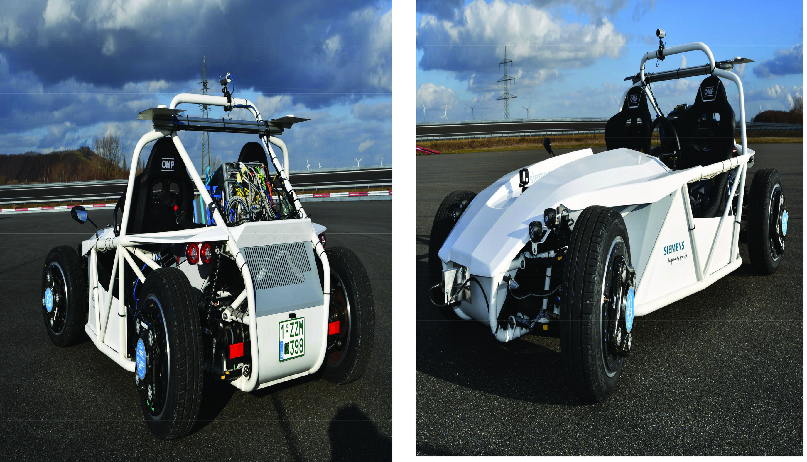
Figure 7 Siemens SimRod test vehicle.
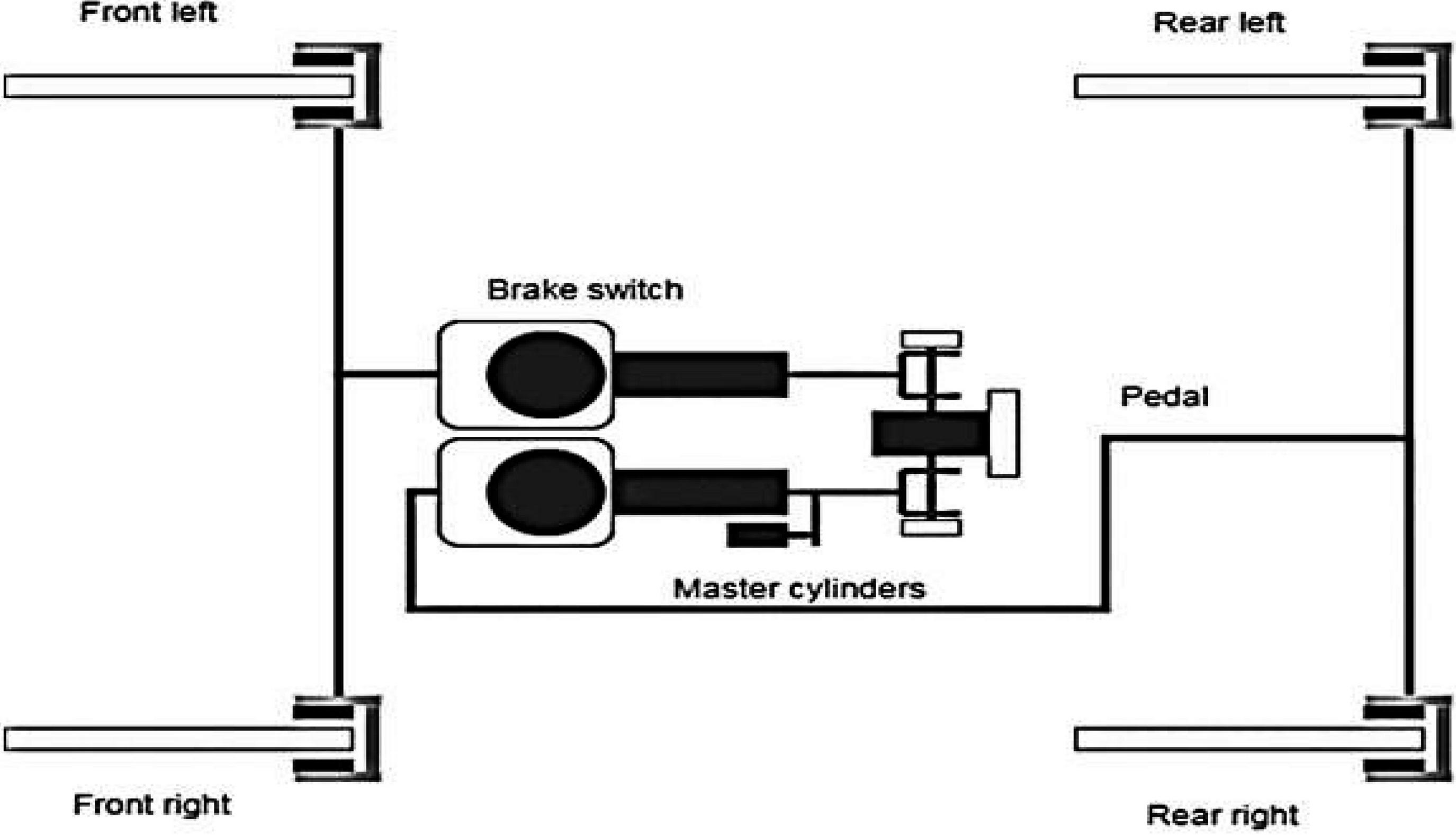
Figure 8 Siemens SimRod brake plant.
For the aim of this work electric regenerative braking was disabled so only the conventional hydraulic brake plant is used to decelerate the vehicle.
SimRod was equipped with the measurement system described in Figure 9:
• Vehicle dynamics and localization: vehicle kinematics and position are identified using a fully integrated OXTSTM RT3003 Inertial Measurement Unit (IMU) (6 D.O.F inertial measurement, GPS and magnetometer);
• Wheel-road interaction: forces exchanged between road and tyres are measured through a 6-axis Wheel Force Transducer (WFT) of the RoaDynTM series, from Kistler; these sensors are installed on wheels;
• Electric drive system: battery and electric drive are continuously monitored, respectively by Battery Management System (BMS) and by Motor Control unit (MCU);
• Additional sensors: vehicle is customized to be easily adapted to different testing activities (a maximum of about 150 signals not fully listed here can be acquired). Also braking plant is monitored by measuring pressures on callipers and brake pedal position.
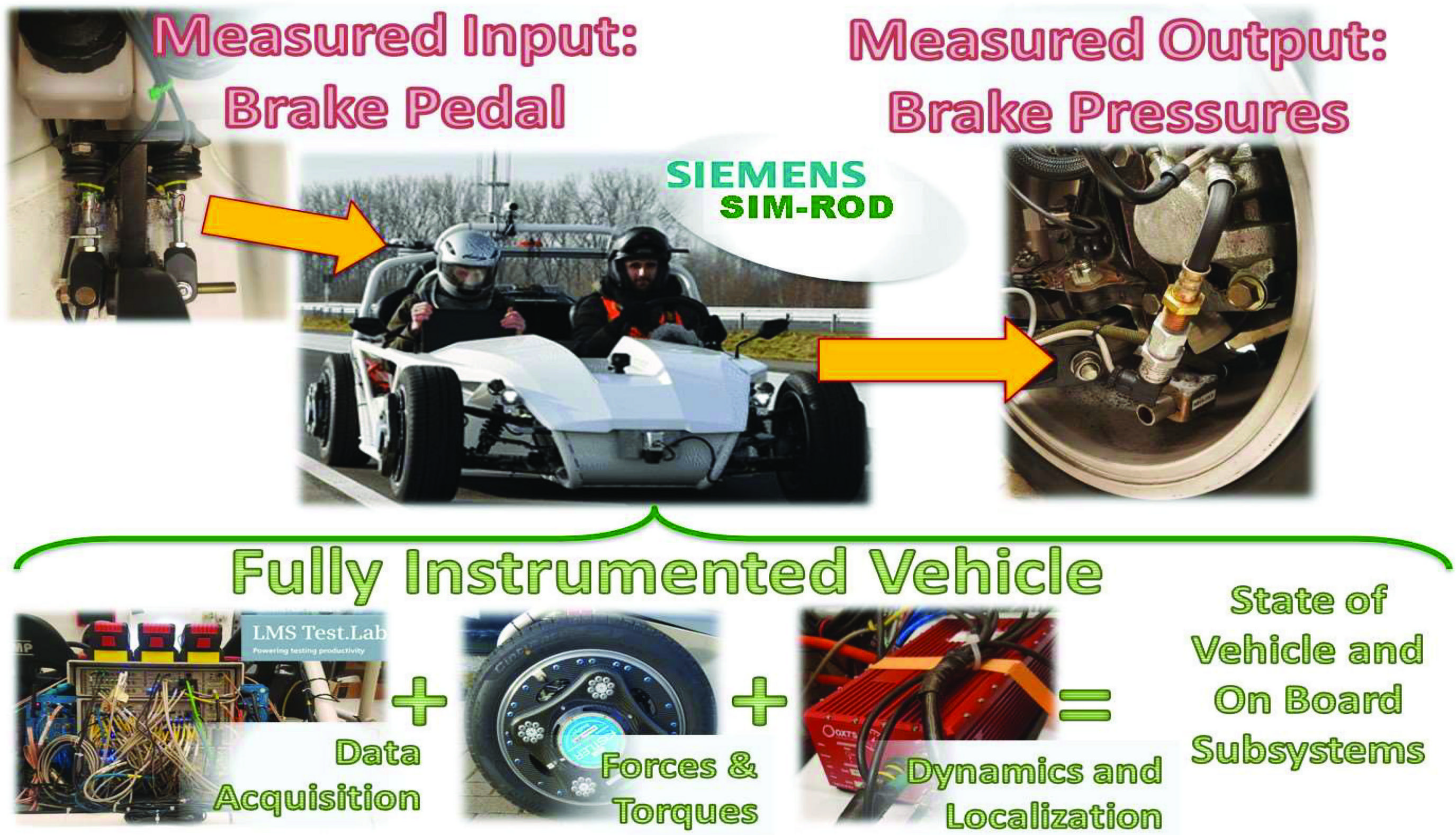
Figure 9 Main elements of the acquisition system installed on SimRod prototype for the identification of main brake plant features.
All data are collected using a Siemens Simcenter SCADAS.
For the particular purpose of this work, hydraulic plant was equipped with additional sensors described in Table 2. All brake related measurements (displacement measures, forces, pressures, etc.) are acquired with a sampling frequency of 1024 Hz.
Brake pedal position is acquired as plant input, while corresponding pressures measured on callipers are acquired as plant outputs. Brake pedal forces are considered as system feedback.
This general approach is applicable to several different kind of brake plants, including brake by-wire ones, in which this kind of signals are often generated by different components and subsystems.
Table 2 Vehicle and brake plant datasheet
| Phis. Quantity | Symbol | Sensor | Measured |
| Force(f) | F | Strain gage | Strain[] |
| Force(r) | F | Strain gage | Strain[] |
| Displ.(f) | x | Potentiometer | Displ.[mm] |
| Displ.(r) | x | Potentiometer | Displ [mm] |
| Pressure.(f) | p | Pressure s. | Pressure[bar] |
| Pressure(r) | p | Pressure s. | Pressure [bar] |
4 Performed Identification Campaign: Methods and Obtained Results
4.1 Aim and Organization of Testing Campaign
Aim of performed campaign is to verify how proposed model can fit the response of a real plant with a reduced set of known data and experimental results.
Test campaign have been organized in the as follow:
• Standstill Tests: to identify the response of the hydraulic brake plant, it is not necessary to have the vehicle in motion. So, tests have been performed in standstill conditions (vehicle not running); known inputs are applied to brake pedals, to identify hydraulic plant behaviour, in terms of clamping pressure inside callipers. Model proposed by UNIFI implements a decoupled scheduling of both amplitude and frequency response of brake plant.Thanks to this approach, it was possible to calibrate separately the model first in terms of amplitude response with steady state tests, refining aspects related to frequency response with few dynamic tests:
∘ Amplitude Response Identification: aim of these tests is to find a relationship between the input position of the pedal and the steady state response in terms of braking pressure. Real plants suffer of hysteresis effects. So tests have been repeated considering both rising and falling behaviour of brake command signals. To perform identification of amplitude response, two kind of inputs waveforms should be considered:
■ Three-Steps Signals: a multiple steps signals (rising and falling) whit smooth ramps.
■ Single Step Signals: a slope which are negligible respect to the transient response of the investigated systems.
∘ Frequency Response Identification: to identify the frequency response of the plant a wide spectrum must be excited. Real systems are truly non-linear. So, identification of frequency response (which suppose a linear behaviour) must be performed locally around a well-known working point. For fluid systems, non-linear behaviour is also influenced not only by the value of considered states (pressure and flow), but also by their derivatives. This behaviour is quite common for electro-mechanical [33] and electro-hydraulic actuators [34]. Internal frictions influence actuator response in terms of exerted torque/forces. Friction and more generally hysteretic effects are strongly influenced by sign of traveling speed in four quadrant operations. The simplest way to produce a wide excitation over different working conditions is represented by multi-step tests (composed by rising and falling edges). This is a clear advantage of the proposed procedure since the same kind of test should be used to perform model tuning both in terms of amplitude and frequency response. Further tests should be obtained also with different waveforms, however in this work procedure was deliberately simplified as much as possible.
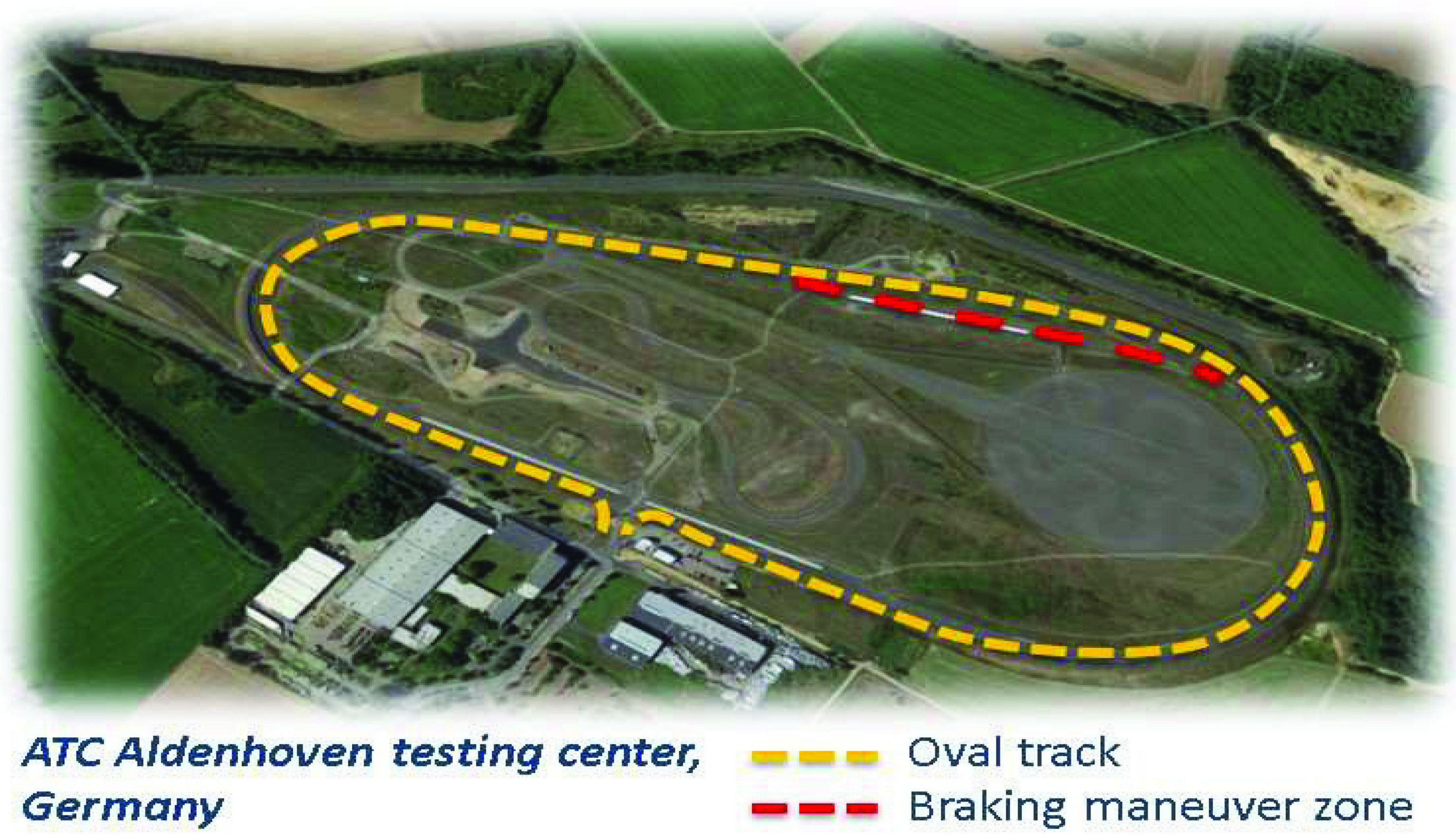
Figure 10 Testing center of Aldenhoven (Germany).
• Dynamic Test on Circuit: model calibration is substantially performed with previously described multi-step tests. So, authors execute some additional tests to perform a preliminary validation of the model with the vehicle running on a circuit. Purpose of this activity is to verify how various braking patterns performed on a circuit by a driver should be fitted by a model calibrated with a limit number of step test in standstill conditions. These additional tests have been performed on the circuit of Aldenhoven (Germany). Tests were performed on a dedicated ”Braking manoeuvre zone”, visible in Figure 10. Braking tests have been executed in a special section of the circuit specifically designed and certified to assure a stable asphalt-tire friction coefficient (more than 0.9). In this way the possibility of adhesion losses during performed tests is excluded. These Experimental runs are of limited interest for the identification of hydraulic brake plant, but are quite useful, at least, to validate corresponding braking torques and longitudinal forces. In this work their usage is still relatively limited: these tests are mainly used to roughly verify the proportionality between clamping pressures and corresponding braking forces, but they are of fundamental importance for further research activities, that should be presented in future publications.
4.2 Amplitude Response Identification
Static tests are performed with the vehicle in standstill conditions and with disabled regenerative braking. In order to identify the amplitude response of plant, authors execute some simple tests: first, brake pedal is lowered slowly (imposing a linear displacement growth), in order to identify the dead-band or some compliance that has to be recovered in terms of pedal displacements. In this way is possible to produce a non-zero response of the plant, in terms of brake pressure.Values of identified compliance for both front and rear brakes, in terms of brake pedal runs, are substantially the same.Then test with multiple braking tests are executed: brake pedal position (input) is imposed and corresponding pressures on callipers (outputs) are measured. In Figure 11 imposed pistons run profile is shown: in each test brake pedal position is increased from the lower end run to the upper one, with three consecutive steps. Amplitude of each intermediate step is randomly perturbed and their duration is high enough to assure the achievement of steady state conditions before the application of the following step (the duration of t is much bigger than the observed time constant of the system). Multiple micro-steps or ramps should be applied during each macro-step, to better identify specific plant features, whose time constant is far lower than the one previously investigated. After maximum run is reached pedal returns to the lowest position through three falling steps that are generated with the same random procedure used for the rising ones. Displacements of rear and front master cylinders are proportional since there are connected by a leverage. This cycle is repeated for at least ten times to have data corresponding to a population of at least 60 random steps (30 rising and 30 falling steps). Additional single step tests are also performed to verify the system behaviour for some specific manoeuvres. A summary of the performed tests (also considering different response of rear and front brakes) are shown in Table 3.
To calibrate the scheduled relation between pedal displacement and corresponding steady state pressure of brake plant, it is recommended to observe the system output after transient becomes negligible. In Figure 11 is visible an example of this procedure: when derivatives of observed signals are sufficiently low, we perform a running mean of the observed pressure. In this way, as visible in Figure 12, it is possible to evaluate two interpolated curves for the rising and falling values of the reference, that approximately describe the amplitude response of the system, including its hysteresis. In particular, according to the sign of Brake, it’s possible to define an upper rising gain profile and a falling one. Results of Figure 13 are scaled respect to maximum input displacements and maximum brake pressure of front and rear callipers, respectively.

Figure 11 Experimental three-steps input measurement results: imposed brake piston displacements.
Table 3 Different identification tests executed on the system
| Test Name | Pressure Range [bar] | |
| Front | Rear | |
| 3 Steps | 0-31 | 0-21 |
| Single Step | 0-68 | 0-49 |
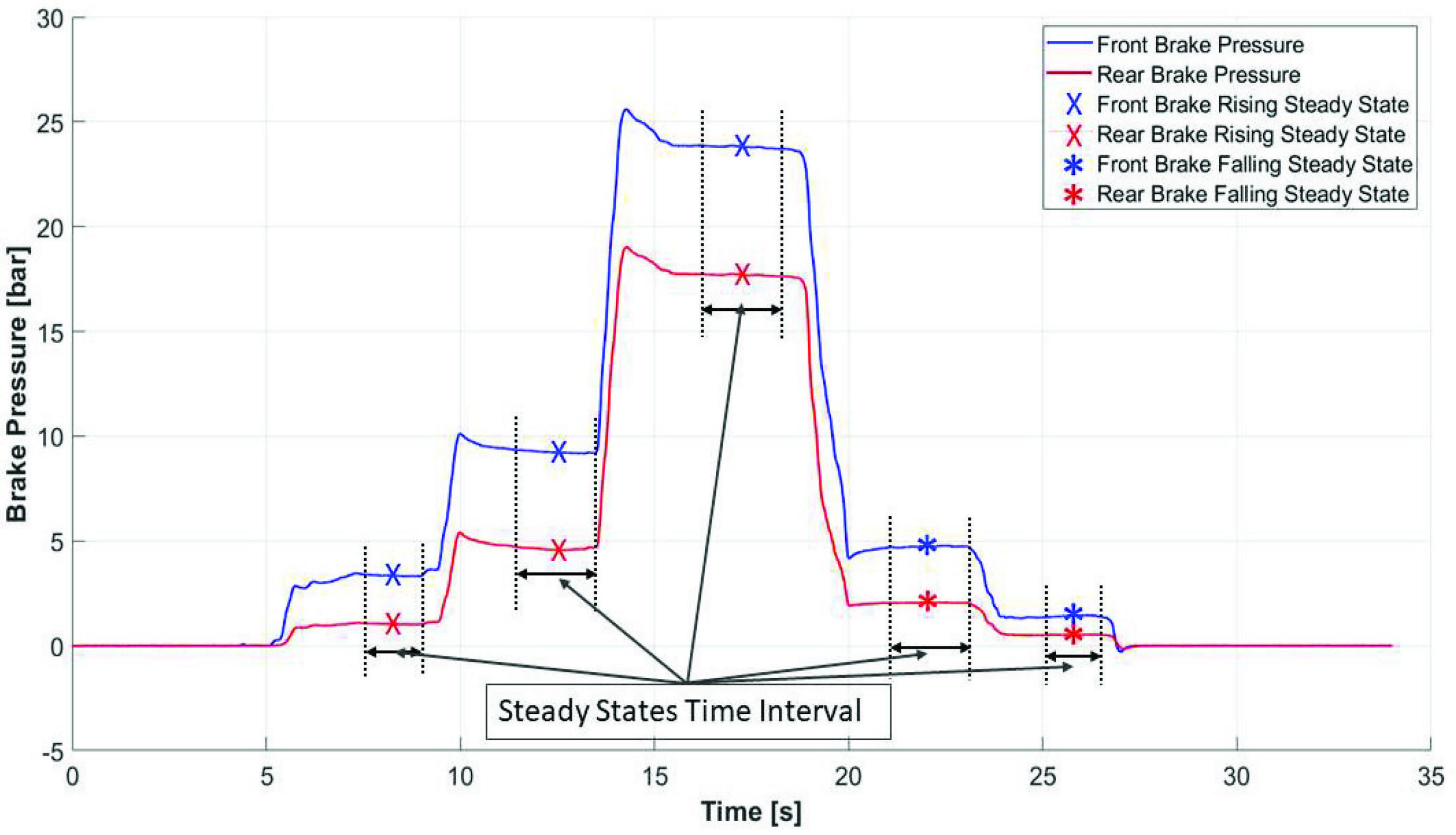
Figure 12 Evaluation of steady-state values for a three-steps test: brake pressures.
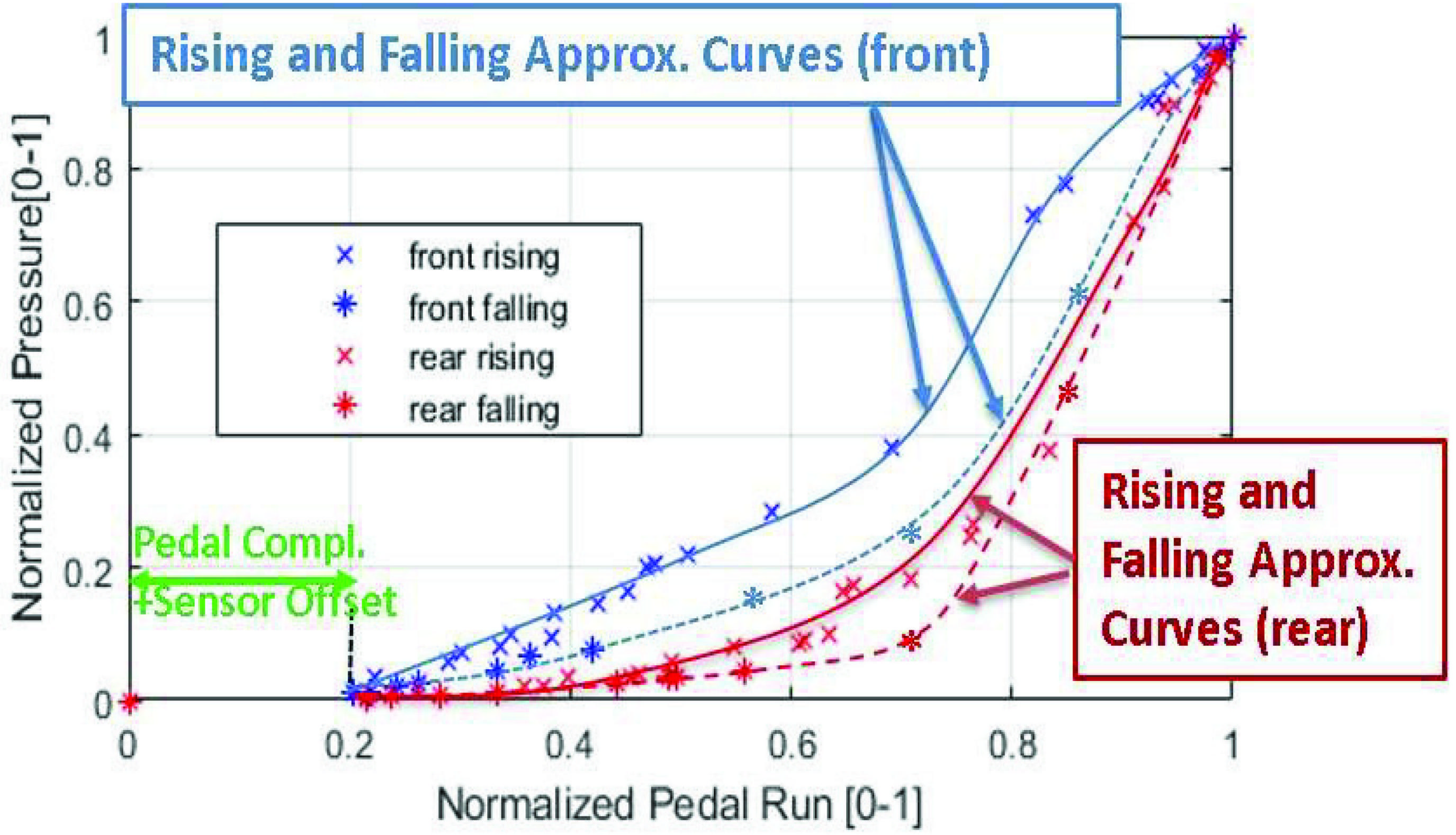
Figure 13 Normalized pressure plant response vs. normalized pedal run.
4.3 Frequency Response Identification
As visible in Figure 8, tested vehicle is not equipped with ABS or other device aiming to modulate braking forces when degraded adhesion conditions occurs. So, in this vehicle brake cylinders are directly connected to master cylinders. Main parameters of pipes and callipers are known. So, the only parameters that have to be tuned, to fit plant response, are and of the second order transfer function (4). This transfer function describes the dynamic behaviour between brake pedal command and corresponding pressures delivered to callipers. In this test case this functionality is performed by master cylinders. To fit experimental response of the plant, and should be scheduled respect to measured inputs or states and their corresponding derivatives: coefficients of (4) are scheduled respect to the sign of the derivatives of Brake and P, as described in Table 4. Frequency calibration is performed on the same kind of step tests described in Table 3, that have been used to for the previous calibration of system amplitude response. Coefficients of Table 4 have been calibrated manually after few iterations, to fit as possible experimental results of calibration step tests. Since experimental data were naturally noisy pressure and brake command derivatives must be calculated with a relatively aggressive filtering (Butterworth 3rd order with a cutting frequency of about 100 rad/s). This treatment of measured signals proved to be one of the major sources of errors in performed activities.
Table 4 Vehicle and brake plant datasheet
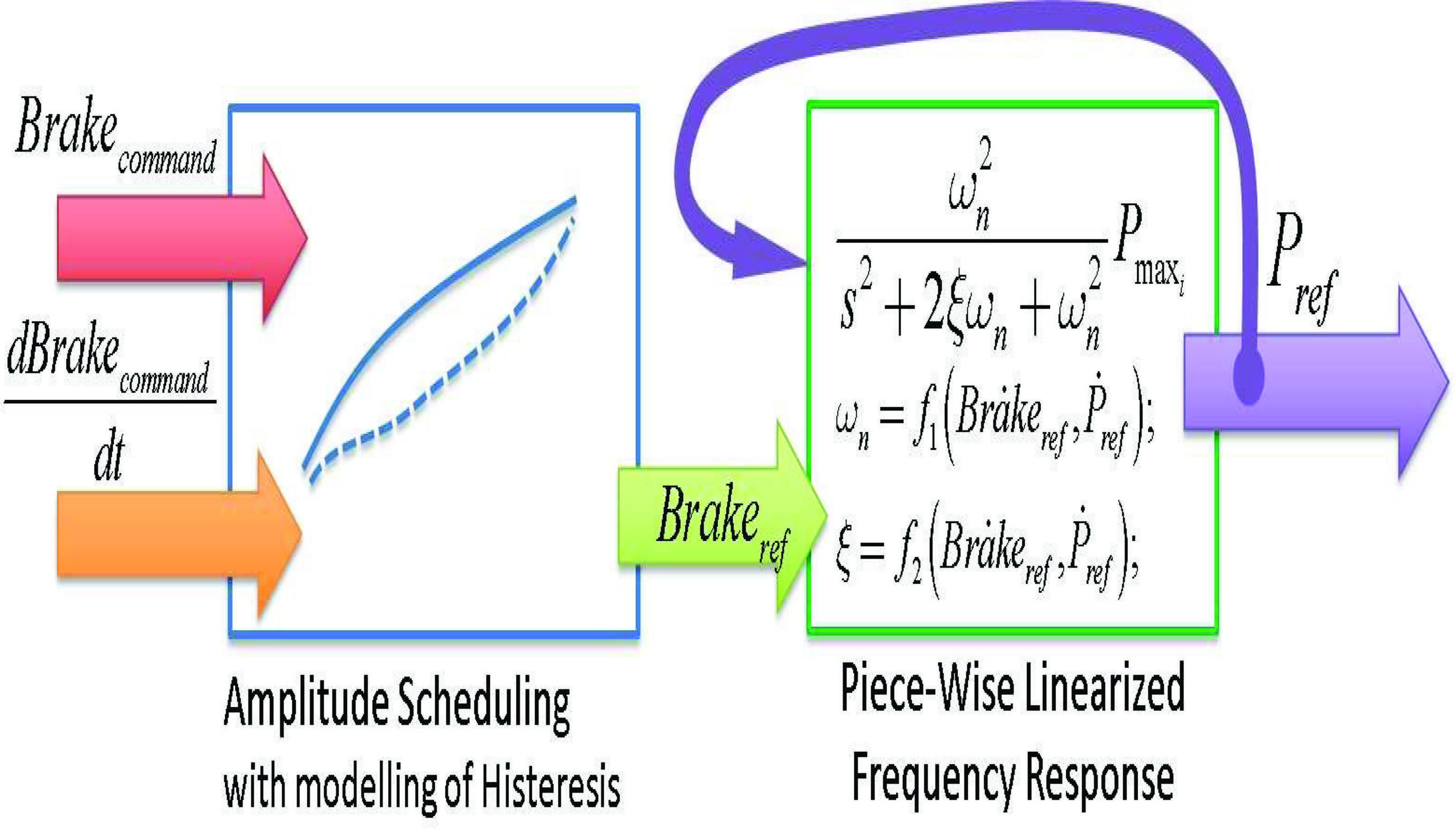
Figure 14 Application of ampl. and freq. scheduling to the brake command signal.
4.4 Calibration Tests, Some Examples
By applying both over explained amplitude and frequency scheduling described in Figure 14, authors were able to fit in quite satisfying way experimental behaviour of calibration tests. In Figure 15 proposed model, even with the simple manual calibration, can reproduce some typical non-linearity of performed step tests: results are very good especially for step tests in which brake effort is applied, otherwise in case of brake release, errors between simulated and measured pressures are a bit higher. These higher errors on release tests are probably due to calibration and modelling of hysteretic phenomena which should be further refined. Source of higher error is mainly the correct recognition of the sign of derivatives as described in Table 4. On a real noisy signal, derivatives of brake commands and pressures are affected by relatively high errors that must be filtered so overexplained recognition of hysteretic effects should less precise than expected. Step Tests like the one described in Figure 15 have been performed considering different values of brake pressures and different sequences of performed brake and release steps.

Figure 15 Example of fitting performance of the brake model with respect to experimental results on three steps (3 rising steps and 3 decreasing steps, measurement referred to front wheels) tests used during calibration tests.
Table 5 Evaluation of additional step tests performed during the calibration phase
| Max Abs | Max Rel. | Max Slope | |||
| Test | Max Pressure | ErrorFront// | ErrorFront// | Delay*Front// | |
| N. | Type | Front//Rear | Rear | Rear | Rear |
| 1 | Single Step | 47.7[bar]//35[bar] | 3.1[bar]//4.2[bar] | 6.5%//12% | 63[ms]//142[ms] |
| 2 | Single Step | 51.2[bar]//36.9[bar] | 4.2[bar]//3.1[bar] | 8.2%//8.4% | 51[ms]//123[ms] |
| 3 | Single Step | 61.1[bar]//46.7[bar] | 2.2[bar]//3.6[bar] | 3.6%//7.7% | 89[ms]//87[ms] |
| 4 | Single Step | 61.1[bar]//46.7[bar] | 3.5[bar]//5.1[bar] | 5.7%//11.1% | 41[ms]//52[ms] |
| 5 | Single Step | 61.4[bar]//46[bar] | 3.9[bar]//3.4[bar] | 6.7%//7.4% | 63[ms]//63[ms] |
| 6 | Single Step | 62.5[bar]//48[bar] | 3.5[bar]//5.3[bar] | 5.6%//11% | 52[ms]//42[ms] |
| 7 | Single Step | 60.8[bar]//48.8[bar] | 3.1[bar]//4.1[bar] | 5.1%//8.4% | 78[ms]//86[ms] |
| 8 | Single Step | 64.4[bar]//47[bar] | 2.9[bar]//3.7[bar] | 4.5%//7.9% | 143[ms]//78[ms] |
| 9 | Single Step | 59.2[bar]//40.9[bar] | 4.5[bar]//2.9[bar] | 7.6%//7.1% | 32[ms]//96[ms] |
| 10 | Single Step | 68.5[bar]//49[bar] | 3.7[bar]//2.5[bar] | 5.4%//5.1% | 69[ms]//113[ms] |
| 11 | Single Step | 61.2[bar]//47.3[bar] | 4.1[bar]//3.5[bar] | 6.7%//7.4% | 87[ms]//105[ms] |
| 12 | 3-Step | 26.8[bar]//16[bar] | 1.5[bar]//1.5[bar] | 5.6%//9.4% | 35[ms]//132[ms] |
| 13 | 3-Step | 14.3[bar]//9[bar] | 2.8[bar]//1.8[bar] | 19.6%//20% | 42[ms]//69[ms] |
| 14 | 3-Step | 14.4[bar]//8[bar] | 1.5[bar]//2.2[bar] | 10.4%//27.6% | 41[ms]//78[ms] |
| 15 | 3-Step | 13.4[bar]//8[bar] | 1.7[bar]//2.3[bar] | 12.7%//28.8% | 63[ms]//84[ms] |
As visible in Table 5 tests are performed considering a single sequence of brake and release manoeuvre or a sequence of three incremental braking steps followed by three release steps as described in Figure 15. Results in Table 5 are mainly evaluated according the following performance criteria:
• Maximum errors between simulated results and experimental measurements in terms of absolute and relative errors.
• Delay of the maximum gradient on release manoeuvres: as previously introduced in example of Figure 15: both on simulated results and experimental data is evaluated the position of an inflected point in which gradient of brake pressure profile reach a local maximum value. This point corresponds to an inflection point of rising or falling profiles of brake pressure. On both curves (simulated results and exp. data) these inflection points are evaluated then it is calculated the time delay (the difference in terms of time) between them. Aim of this performance index is to evaluate how response of the proposed model should be delayed respect to experimental data when transients do to step excitations occurs. Higher errors are due to the difficult detection of hysteretic phenomena during the transition between braking and release manoeuvres since this evaluation must be performed observing local derivatives which have to be filtered to avoid noisy performances. This trouble causes a delay visible in Figure 15 (this example was chosen as “worst case” among others to make more evident this effect) between measured and simulated pressure profiles. This delay is measured comparing the time-distance between points in which a stable maximum gradient pressure derivative is reached during the manoeuvre. Brake steps test have been performed by human drivers this introduce a certain variability on applied brake pedal commands that helped the authors to perform a more robust calibration.
Since errors on brake application manoeuvres are far lower this maximum delay is always measured as in the example of Figure 15 in a brake release phase.
These evaluation criteria have been chosen to make more evident the effect of errors on transients since errors on steady state values were much lower.
For what concern the choice of performed test authors performed many “single step” brake tests (tests 1–11 in Table 5) in which a relatively high effort is applied and then after 5–10 seconds is released. Then to better calibrate the model with low brake efforts, three step tests like the one of Figure 15 are repeated for lower pressure levels (tests 12–15 in Table 5).
From results of Table 5 it should be deduced that maximum errors in terms of simulated pressures are limited to few bars (typically around 2–2.5 bars). However, it should be considered that repeatability of brake tests involves fluctuations on measured exp. Pressures of about 1 bar. Also it should be considered that these high errors are recorded during the brake release phase; also in this case delays measured on the real plant are affected by repeatability errors of about 100 [ms] so it should be concluded that modelling errors are only a bit higher respect to random variations that can be observed on the real plant.
5 Validation: Preliminary Results
For the validation process, SimRod vehicle was transported to the test circuit of Aldenhoven, where it was possible to perform various manoeuvres at different speed. In this occasion it was possible to measure both brake pedal runs and corresponding brake pressures. By imposing the same recorded input to the calibrated model of the brake plant, it was possible to compare the simulation results respect to corresponding brake pressures measured during the experimental activities. In Figures 16, some of these comparisons, which are referred to relatively complex brake manoeuvres, are shown: considering the simplicity of the proposed model and the difference between the experimental profiles and the calibration ones, obtained results are very good in terms of fitting capability. As previously described in Section 4, higher errors are mainly due to the modelling of hysteretic effects since results are relatively sensitive to the way in which state derivatives of pressure and brake command described in Table 4 are evaluated: currently these derivatives are directly evaluated after the application of low pass filters (Butterworth 3rd order ) with a cutting frequency of about 100 rad/s (about 16 Hz). These relatively aggressive filtering must be introduced to avoid high frequency noise which disturbs a proper estimation of derivatives, but it is also the reason of errors and delays in detecting hysteretic effects.
Further validation results are shown in Figures 17–19: vehicle is accelerated to a speed of about 24.5 m/s, then the brake is activated, and vehicle is stopped with four seconds.
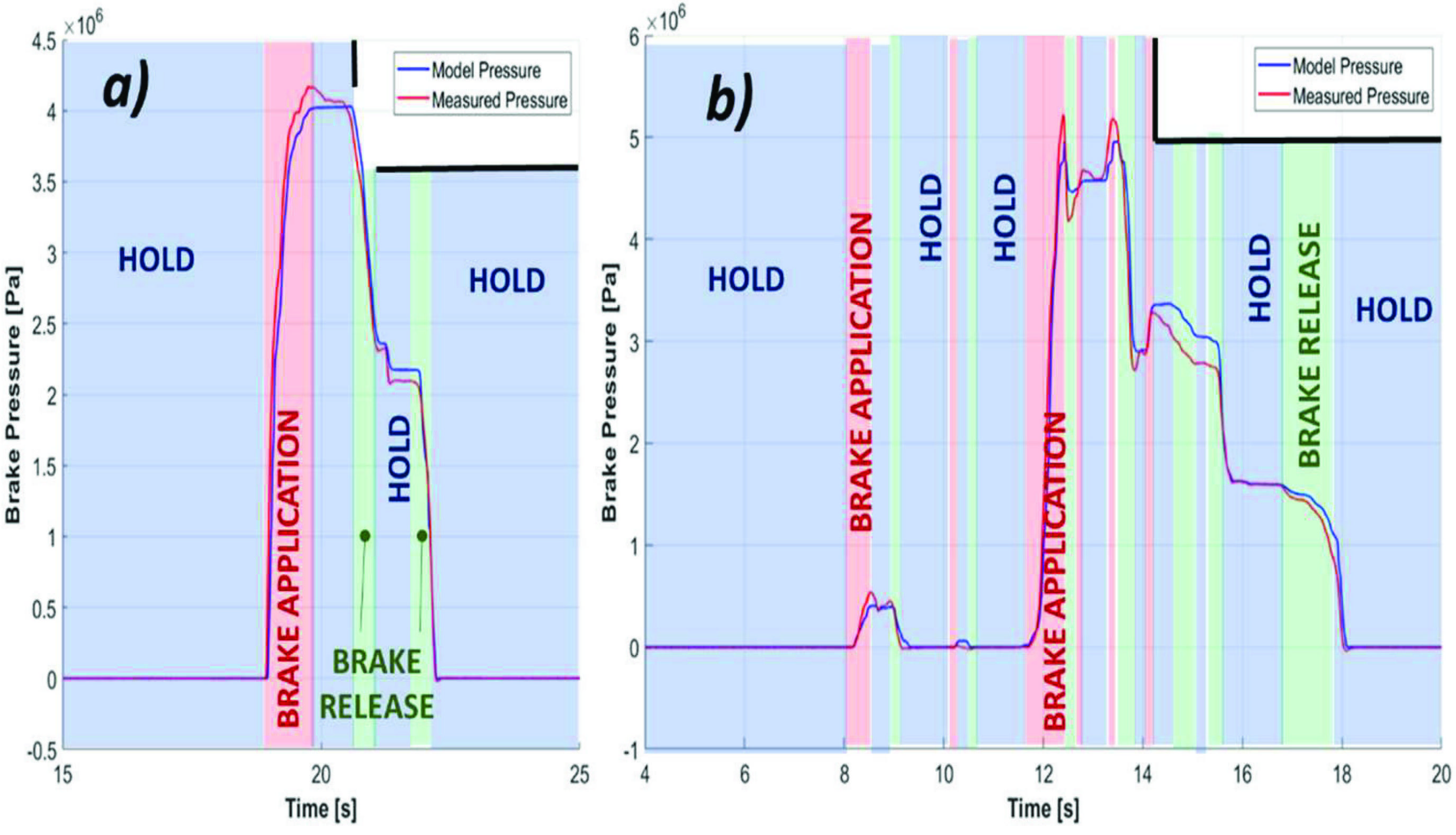
Figure 16 (a/b) Example of fitting performances of brake model respect to real experimental results measured during real braking manoeuvre performed on the test circuit of Aldenhoven (tests are referred to various braking manoeuvre performed at 50 and 60 km/h).

Figure 17 Comparison of measured and simulated brake pressure during a braking test (simulated results are obtained imposing the same brake pedal displacement).
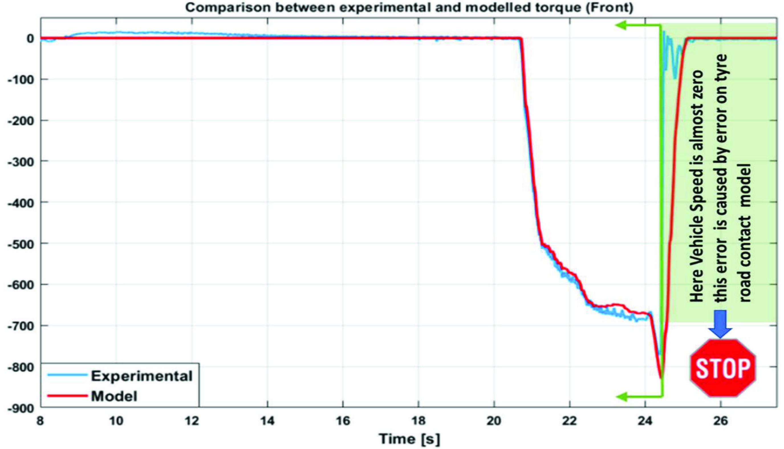
Figure 18 Comparison of measured and simulated torque profiles during a braking test (simulated results are obtained imposing the same brake pedal displacement).
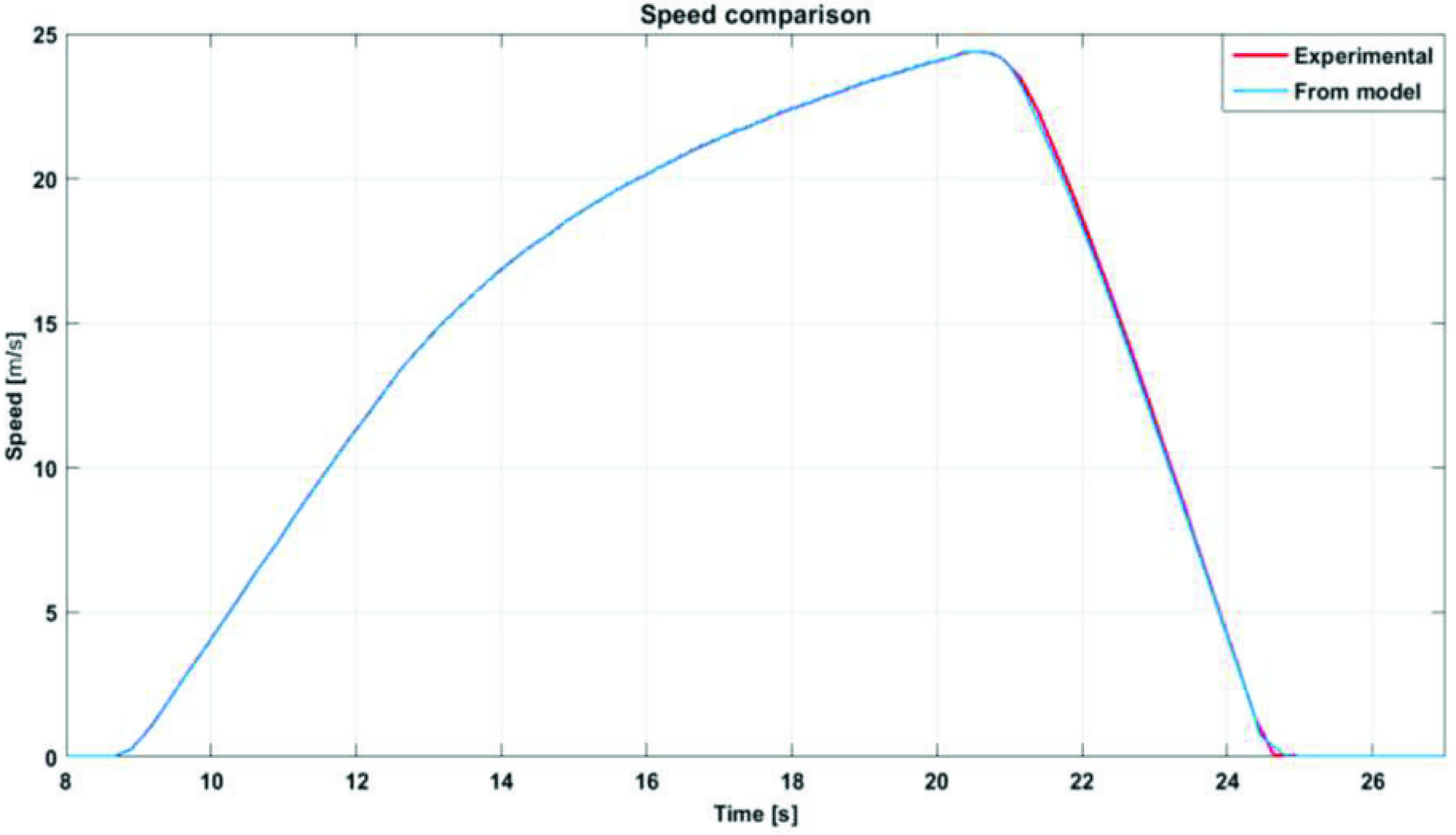
Figure 19 Comparison of measured and simulated vehicle speed profiles during a braking test (simulated results are obtained imposing the same brake pedal displacement.
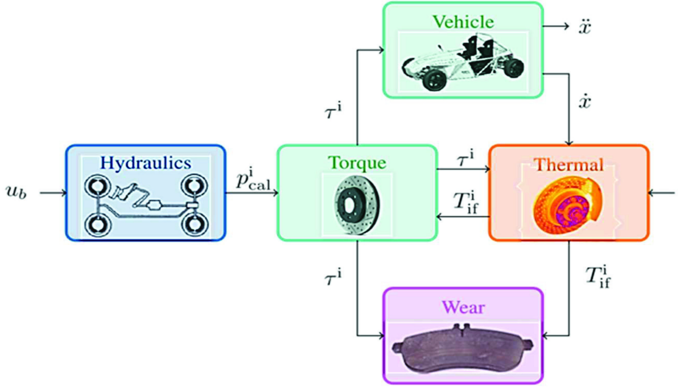
Figure 20 Full vehicle model adopted for the evaluation of vehicle speed profile [38].
Adopted vehicle model includes also the simulation of brake friction materials as described in Figure 20; for a detailed description of vehicle model it’s recommended the lecture of a recent work [38] whose content was not inserted in this work to avoid an excessive paper length. Vehicle model implemented in Matlab Simulink includes a simplified vehicle dynamic (including a simplified Pacjeka model of wheel-road interaction), a scheduled friction model for brake pads which take count also of thermal aspects.
In Figure 17 simulated brake pressure (on front wheel) are compared with experimental ones (the same brake pedal command is imposed in both cases); knowing the friction factor of the pad simulated brake pad torques are compared with corresponding experimental torque measurements (wheels of Simrod are also equipped with force and torque sensors) as shown in Figure 18. For what concern torque applied to wheels, some appreciable difference between simulated torque and recorded one is recognizable only when the vehicle is completely stopped: Since error on brake plant pressure (Figure 17) is very low it should be argued that for very low vehicle speed (10/10 m/s) resulting error on torques visible in Figure 18 are mainly due to numerical problems of the road-tyre contact model. This is a common situation since for a null vehicle speed calculation of road tyre slip is often ill conditioned.
Finally, by applying the simulated torques to a mechanical model of the vehicle, it’s possible to calculate the corresponding speed profile of the car-body, which is compared in Figure 19 with corresponding experimental value.
Looking at results of Figures 17–19 it’s clearly noticeable that brake pressure profiles are well reproduced: in particular errors in terms of brake pressure didn’t produce appreciable variations not only in terms of torques but also in term of vehicle speed profile which mainly depends from integral of braking actions. So, it should be further concluded that recorded errors in terms of braking torques are quite acceptable to properly reproduce vehicle dynamical behaviour.
6 Conclusions and Future Developments
In this work, authors have proposed a simplified brake model designed to fit the functional behaviour of different brake plants. The model has been applied on a benchmark test vehicle (Siemens SimRod) for which it was not originally designed, proving to be able to fit the real behaviour of a brake plant through a limited set of experimental tests. Also, preliminary validation results obtained on a test circuit are quite encouraging. Results clearly indicate that brake pressures are reproduced quite precisely, and recorded errors produce negligible errors in terms of simulated vehicle dynamics.
Residual errors recorded in the comparison of experimental data with simulation results are compatible with signal conditioning of acquired signals and consequent troubles in calculation of state derivatives, so there are also margins for future improvements of proposed methods by introducing a more sophisticated handling of pressure and brake command derivatives.
For future activities, it is planned a better identification of parameters dealing with the calculation of applied braking forces (e.g. friction factor) and a more sophisticated integration of the current brake plant model with the regenerative brake and vehicle’s dynamics. For what concerns other vehicles and brake plants (different from the Kyburz SimRod),planned future activities will be focused on the calibration of the same brake model to the other UC, proposed by the other partners of OBELICS project. Finally, further modelling improvements should be introduced to simulate degraded performances of the plant, that should be associated to known failure modes or functional degradation of the plant. This last possible improvement is strictly connected to the aims of OBELICS project: providing to product designers tools useful to verify resiliency, robustness and more generally safety of the proposed systems, respect to undesired or degraded working conditions. Additional evaluations in terms of maximum estimated delays between rising front of front and rear brakes are also introduced. Current results are encouraging, considering the limited amount of performed calibration tests. For all these reasons authors are quite confident of being able to drastically improve obtained results within few months of activity.
Finally authors are also considering to extend the adopted modelling approach based on scheduled transfer function also to model needed to plan vehicle trajectories extending methodologies currently proposed for railway applications [39].
Acknowledgements
This project has received funding from the European Union’s Horizon 2020 research and innovation program under grant agreement No 769506.
References
[1] Gerdes JC, Hedrick JK. Brake System Modeling for Simulation and Control. Journal of Dynamic Systems, Measurement, and Control 1999; 121: 496–503.
[2] Delaigue P, Eskandarian A. A comprehensive vehicle braking model for predictions of stopping distances. Proceedings of the Institution of Mechanical Engineers, Part D: Journal of Automobile Engineering 2004; 218: 1409–1417.
[3] Savitski D, Ivanov V, Augsburg K, et al. The new paradigm of an anti-lock braking system for a full electric vehicle:experimental investigation and benchmarking. Proceedings of the Institution of Mechanical Engineers, Part D: Journal of Automobile Engineering 2016; 230: 1364–1377.
[4] Ming L. Kuang. Hydraulic brake system modeling and control for active control of vehicle dynamics. In: Proceedings of the 1999 American Control Conference (Cat. No. 99CH36251). San Diego, CA, USA: IEEE, pp. 4538–4542 vol. 6.
[5] Anselma PG, Patil SP, Belingardi G. Rapid Optimal Design of a Light Vehicle Hydraulic Brake System. pp. 2019-01–0831.
[6] Bauer F, Fleischhacker J. Hardware-in-the-Loop Simulation of Electro-Pneumatic Brake Systems. pp. 2015-01–2745.
[7] Li L, Li X, Wang X, et al. Transient switching control strategy from regenerative braking to anti-lock braking with a semibrake-by-wire system. Vehicle System Dynamics 2016; 54: 231–257.
[8] Zhang J-Z, Chen X, Zhang P-J. Integrated control of braking energy regeneration and pneumatic anti-lock braking. 224: 24.
[9] Miller JM. Electric Powertrain: Energy Systems, Power Electronics and Drives for Hybrid, Electric and Fuel Cell Vehicles [Book Review]. IEEE Power Electron Mag 2018; 5: 86–87.
[10] Enang W, Bannister C. Modelling and control of hybrid electric vehicles (A comprehensive review). Renewable and Sustainable Energy Reviews 2017; 74: 1210–1239.
[11] Fagnant DJ. Preparing a nation for autonomous vehicles: opportunities, barriers and policy recommendations. 2015; 15.
[12] Gonzalez D, Pérez J, Milanés V, et al. A Review of Motion Planning Techniques for Automated Vehicles. IEEE Transactions on Intelligent Transportation Systems 2016; 17: 11.
[13] Amer NH. Modelling and Control Strategies in Path Tracking Control for Autonomous Ground Vehicles: A Review of State of the Art and Challenges. J Intell Robot Syst 2017; 30.
[14] Berzi L, Favilli T, Locorotondo E, et al. Real Time Models of Automotive Mechatronics Systems: Verifications on “Toy Models”. In: Carbone G, Gasparetto A (eds) Advances in Italian Mechanism Science. Cham: Springer International Publishing,pp. 141–148.
[15] Pugi L, Favilli T, Berzi L, et al. Brake Blending and Optimal Torque Allocation Strategies for Innovative Electric Powertrains. In: Saponara S, De Gloria A (eds) Applications in Electronics Pervading Industry, Environment and Society. Cham: Springer International Publishing, pp. 477–483.
[16] Pugi L, Favilli T, Berzi L, et al. Application of Regenerative Braking on Electric Vehicles. In: 2019 IEEE International Conference on Environment and Electrical Engineering and 2019 IEEE Industrial and Commercial Power Systems Europe (EEEIC/ICPS Europe). Genova, Italy: IEEE, pp. 1–6.
[17] Zhao X, Li L, Wang X, et al. Braking force decoupling control without pressure sensor for a novel series regenerative brake system. Proceedings of the Institution of Mechanical Engineers, Part D: Journal of Automobile Engineering 2019; 233: 1750–1766.
[18] Han W, Xiong L, Yu Z. A novel pressure control strategy of an electro-hydraulic brake system via fusion of control signals. 16.
[19] Ma, L.-X., Yu, L.-Y., Wang, Z.-Z., Song, J. A new type of automotive braking actuator for decentralized electro-hydraulic braking system(2014) Journal of Harbin Institute of Technology (New Series), 21 (1), pp. 1–6.
[20] Zhang J, Lv C, Gou J, et al. Cooperative control of regenerative braking and hydraulic braking of an electrified passenger car. Proceedings of the Institution of Mechanical Engineers, Part D: Journal of Automobile Engineering 2012; 226: 1289–1302.
[21] Aly, A. A., Zeidan, E. S., Hamed, A., Salem, F. (2011). An antilock-braking systems (ABS) control: A technical review. Intelligent Control and Automation, 2(03), 186.
[22] Pugi L, Rindi A, Ercole AG, et al. Preliminary studies concerning the application of different braking arrangements on Italian freight trains. 28.
[23] Pugi L, Malvezzi M, Papini S, et al. Simulation of braking performance: The AnsaldoBreda EMU V250 application.Proceedings of the Institution of Mechanical Engineers, Part F: Journal of Rail and Rapid Transit 2015; 229: 160–172.
[24] Wang X, Zheng G. Two-step transfer function calculation method and asymmetrical piecewise-linear vibration isolator under gravity. Journal of Vibration and Control 2016; 22: 2973–2991.
[25] Rewienski M, White J. A trajectory piecewise-linear approach to model order reduction and fast simulation of nonlinear circuits and micromachined devices. IEEE Trans Comput-Aided Des Integr Circuits Syst 2003; 22: 155–170.
[26] Pugi L, Galardi E, Carcasci C, et al. Preliminary design and validation of a Real Time model for hardware in the loop testing of bypass valve actuation system. Energy Conversion and Management 2015; 92: 366–384.
[27] Yu L, Liu X, Xie Z, et al. Review of Brake-by-Wire System Used in Modern Passenger Car. In: Volume 3: 18 International Conference on Advanced Vehicle Technologies; 13th International Conference on Design Education; 9th Frontiers in Biomedical Devices. Charlotte, North Carolina, USA: American Society of Mechanical Engineers, p. V003T01A020.
[28] Karnopp D, Margolis DL, Rosenberg RC. System dynamics: modelling and simulation of mechatronic systems. 5th ed. Hoboken, NJ: Wiley, 2012.
[29] Genta G and Morello L (2007) L’ autotelaio 1 and 2. Torino: Libreria universitaria levrotto and bella.
[30] W. J. Thayer Transfer Introduction Functions for Moog Servovalves. Moog technical bulletin 103 of Moog Inc. available on line at \urlhttp://www.moogvalves.com/
[31] Merrit, H. E. “Hydraulic Control Systems, Jonh Wiley & Sons Inc.” New York ISBN 471596175 (1967).
[32] Yoshida, F., & Miyakawa, S. (2011). Effect of parameters on frequency characteristics of proportional control valve using tap water. In Proceedings of the 8th JFPS International Symposium on Fluid Power, Okinawa, Japan.
[33] Day TD, Roberts SG. A Simulation Model for Vehicle Braking Systems Fitted with ABS. pp. 2002-01–0559.
[34] van Zanten AT. Bosch ESP Systems: 5 Years of Experience. SAE International. Epub ahead of print 2000. DOI: 10.4271/2000-01-1633.
[35] Kant B. Sensotronic brake control (SBC). In: Reif K (ed) Automotive Mechatronics. Wiesbaden: Springer Fachmedien Wiesbaden, pp. 412–415.
[36] Klode H, Omekanda AM, Lequesne B, et al. The Potential of Switched Reluctance Motor Technology for Electro-Mechanical Brake Applications. pp. 2006-01–0296.
[37] Pulcinelli A, Pugi L, Vinattieri F, et al. Design and testing of an innovative electro-hydraulic actuator for a semi-active differential. Proceedings of the Institution of Mechanical Engineers, Part D: Journal of Automobile Engineering 2017; 232: 1438–1453.
[38] D’Hondt, T., Forrier, B., Sarrazin, M., Favilli, T., Pugi, L., Berzi, L., Viviani, R., Pierini, M. Modeling and Identification of an Electric Vehicle Braking System: Thermal and Tribology Phenomena Assessment (2020) SAE Technical Papers, 2020-April (April), DOI: 10.4271/2020-01-109
[39] L. Pugi, A. Reatti, F. Corti and F. Grasso, “A Simplified Virtual Driver for Energy Optimization of Railway Vehicles,” 2020 IEEE International Conference on Environment and Electrical Engineering and 2020 IEEE Industrial and Commercial Power Systems Europe (EEEIC/I&CPS Europe), Madrid, Spain, 2020, pp. 1–6, doi: 10.1109/EEEIC/ICPSEurope49358.2020.9160715
Biographies

Luca Pugi is an associated professor at University of Florence where he is responsible of didactical activities concerning Mechatronics, Electric Traction Systems for Rail and Road Vehicles, Applied Mechanics. Born in 1974 in Florence (Italy) he obtained his degree in mech. Engineering in 1999 at University of Florence (Italy) and discussed his phd thesis in 2003 at University of Bologna (Italy). His current research activities are focused on the application of mechatronics to testing, actuation and control of vehicle systems with a special attention to multidisciplinary networking between research and industrial partners. He is author of more than 200 indexed publications, some patents and winner of several scientific awards for his research activities especially in the railway sector.

Federico Alfatti is a Ph.D. student at the University of Florence. Born in 1994, He received the M.Sc. degree in mechanical engineering from University of Florence, Italy, in 2019. After graduation, he started a Ph.D. on automotive Brake by Wire systems in collaboration with the company Meccanica42. His main research activities are in the field of innovative brake systems for automotive industry, vehicle dynamics, ADAS system, Human in The Loop simulations.

Lorenzo Berzi, Mechanical Engineer, obtained his PhD at the University of Florence in 2013. He is research assistant at the Department of Industrial Engineering of Florence (DIEF) and his main interests concern electric vehicles, innovative mobility and sustainability of materials. As part of the MOVING (Mobility and Vehicle Innovation) Group he has been participating to more than 15 local, national and international research projects.

Tommaso Favilli, born in 1991, graduates in Electrical Engineering in 2018 at University of Florence. Currently is a PhD candidate at the Department of Industrial Engineering of Florence (DIEF). It’s activities are mainly related to road vehicle and real-time simulations, concerning dynamics, stability controller, power management and algorithm’s optimization of onboard controller. Knowledge is acquired in braking system and brake blending strategies for electric vehicles.

Marco Pierini is Full Professor at the Department of Industrial Engineering of Florence (DIEF, University of Florence). He is head and co-founder of the MOVING (Mobility and Vehicle Innovation) Group. He has more than 25 years of experience in transport research with special focus on road safety, vehicle passive and active safety, vehicle electrification, urban and interurban mobility. All the activities are developed at national and international level within national and EC funded projects or in direct cooperation with industry. He has been responsible for more than 30 project at EU, National and regional level.

Bart Forrier was born in Halle, Belgium in 1989. He received the M.Sc.degree in mechanical engineering from KU Leuven, Belgium, in 2011.
After graduation, he first joined LMS Intl., Leuven, Belgium, and laterworked in the Noise & Vibration Research Group at KU Leuven. There, heobtained the Ph.D. in engineering sciences in 2018. Since then, he is aresearcher at SISW NV, and a voluntary researcher at KU Leuven.
His main research activities are in model-based system testing and virtual sensing, with a focus on mechatronic powertrain applications.

Thomas D’hondt was born in Aalst, Belgium, in 1993. He received his M.Sc. degree in electromechanical engineering from Brussels Faculty of Engineering, Belgium, in 2016. Since then, he is a research engineer at Siemens Digital Industries Software. His main research activities focus on model-based system testing, with a focus on electric powertrain applications and automated vehicles.

Mathieu M. Sarrazin received in 2009 from the Technical University College of West-Flanders, now called University of Gent Campus Kortrijk, a first Master degree of Engineering (Meng) in Electromechanical/Electrical Engineering. The focus of his master thesis was at that time on the total design concept for a fully electric driven car.
In 2012, he graduated at the University of Leuven with another Master of Science degree in Mechanical Engineering with a specialisation in Automotive.
He is now eight years part of the research team at Siemens Industry Software. In 2014, he received a unique Siemens Technology Award. Currently, he works as Research and Innovation manager and coordinates national and European research projects. His research interest includes hybrid and electrical vehicles, electromechanical drivelines, data driven research, NVH, model-based testing, converter-machine interactions, fault detection, condition monitoring, mechatronics, signal processing, system identification and control strategies.
e-mail: Mathieu.sarrazin@siemens
International Journal of Fluid Power, Vol. 21_2, 169–210.
doi: 10.13052/ijfp1439-9776.2122
© 2020 River Publishers