Control and Performance Analysis of a Digital Direct Hydraulic Cylinder Drive

Niels H. Pedersen¹, Per Johansen^1,*, Lasse Schmidt¹, Rudolf Scheidl² and Torben O. Andersen¹

¹Department of Energy Technology, Aalborg University, Aalborg, Denmark

²Institute of Machine Design and Hydraulic Drives, Johannes Kepler University, Linz, Austria

E-mail: pjo@et.aau.dk

* Corresponding Author

Received 28 January 2019; Accepted 13 December 2019; Publication 07 March 2020

Abstract

This paper concerns control of a digital direct hydraulic cylinder drive (D-DHCD) and is a novel concept with the potential to become the future solution for energy efficient hydraulic drives. The concept relies on direct control of a differential cylinder by a single hydraulic pump/motor unit connected to each cylinder inlet/outlet. The pump/motor unit in this research uses the digital displacement technology and comprises of numerous individually digital controlled pressure chambers, such that the ratio of active (motoring, pumping or idling) chambers determines the machine power throughput. This feature reduces energy losses to a minimum, since the inactive (idling) chambers has very low losses. A single DDM may provide individually load control for several cylinders without excessive throttling due to various load sizes. Successful implementation of the concept relies on proper control of the DDM, which demands a dynamical model that allows for system analysis and controller synthesis. This is a challenging task, due to the highly non-smooth machine behavior, comprising both non-linear continuous and discrete elements. This paper presents the first feedback control strategy for a D-DHCD concept, based on a discrete dynamical approximation and investigates the control performance in a mathematical simulation model representing the physical system.

Keywords: Digital displacement machines, hydraulics, fluid power, direct drive, control, energy efficient.

1 Introduction

Conventional hydraulic cylinder drives are widely used in industry due to their high power-to-weight ratio, but is challenged by their low efficiency, especially at part load operation. The high losses are a result of throttling through utilization of proportional flow control valves used to achieve the desired cylinder operation. Various solutions for improving the efficiency of cylinder drives has therefore been studied, such that hydraulic drives are a viable candidate for future energy efficient actuation systems. One proposed solution where proportional valve flow control is maintained, is through use of an additional valve, allowing for individual pressure chamber control through the separate metering principle Nielsen (2005). Another solution is to introduce an additional intermediate pressure line, allowing for a reduction in throttling losses at lighter loads through switching between active pressure lines Dengler et al. (2011, 2012). An alternative concept is direct pump/motor flow control, where the throttling losses as a result of proportional flow control valves is omitted. Various solution proposals for achieving proportional direct flow control has been presented which are based on variable displacement units, rectifying bridges and/or accumulator solutions Heybroek et al. (2006, 2008), Ivantysynova and Rahmfeld (1998). However, these methods are often either rather complex and/or costly, why low cost alternative solutions has been investigated, e.g. the speed-variable switched differential pump system Schmidt et al. (2015, 2017). Recently emerging solutions based on digital hydraulics is another alternative to increase the energy efficiency through direct flow control M. Heikkilä (2013). This paper investigates a digital hydraulic solution, where the direct pump/motor flow control is achieved through use of the digital displacement technology. The digital displacement machine (DDM) comprises of numerous displacement chambers in a modular construction, where each chamber is individually controlled by electrically actuated on/off valves. The machine enables utilization of three modes (pumping, mo toring and idling), which in full stroke operation may be changed on a stroke-by-stroke basis once per revolution at a fixed angle for each chamber. This way, the committed displacement is determined by the ratio of active cylinders in discrete levels. Since the chamber pressure remains low in idling mode, it entails very low losses and thus high efficiency at part load operation. Additionally, the use of leakage free digital valves provides reliable load holding which is often a major problem for direct drive solutions. For a more detailed description of the digital displacement technology and operation see e.g. Ehsan et al. (1997), Payne et al. (2005), Rampen (2010).

To enhance efficiency of hydraulic systems it is of interest to implement this tech nology, as a substitute for the conventional resistance control, in hydraulic feedback control systems. However, development of the control system is considered a challenging task due to the non-smooth machine behavior. This may explain why state of the art control strategies are often limited to either neglecting the dynamics or predetermine the actuation sequence offline Johansen et al. (2015), Sniegucki et al. (2013), Armstrong and Yuan (2006), Song (2008), Heikkila and Linjama (2013). Model based feedback control strategies has been developed for the digital displacement machine, but has only been considered for a machine either operating solely in pumping or motoring mode Sniegucki et al. (2013), Pedersen et al. (2016, 2017a,b, 2018). Model based feedback control of a combined pump/motor DDM is complicated by the pump and motor impulse responses being different and the decisions being made out of phase. This paper proposes the first model based control strategy for a DDM that may both use pumping and motoring strokes by use of a discrete angle average approximation method. The performance of the control system is investigated through simulation in a non-linear model representing the physical system.

2 System Description and Mathematical Model

To illustrate the digital direct hydraulic cylinder drive concept and developed control strategy, a simplified load system with a single cylinder is considered. The DDM concept allows each pressure chamber to both act as a pump and a motor unit, such that movement of the main cylinder in both direction is possible with a single fixed speed DDM. The D-DHCD concept under consideration is illustrated in Figure 1.

The DDM consist of 8 modules with 5 cylinders in each module, for a total of 40 cylinders. The 8 modules are divided into two banks with 20 cylinders in each bank, where one bank is connected to the main cylinder piston side and the other to the main cylinder rod side. The cylinders in each bank are radially distributed around a common eccentric shaft and the two banks are parallel connected. The chamber size of the cylinders in each bank is matched with the main cylinder area ratio, such that the chamber sizes on the piston side is larger than on the rod side. When extending the main cylinder, the piston side bank may be set to pumping mode, while the rod side bank may be set to motoring mode. When reversing the direction of motion, the piston side bank may be set to motoring m ode and the rod side bank to pumping mode. This way, the drive torque from the electric rotary machine may be reduced by the generated motor torque. Depending on the size of the load, only a fraction of the cylinders in a bank is active in either pumping or motoring mode, while the remaining chambers are set to idle mode. To smooth out the pressure spikes induced by the digital machine, damping accumulators is placed in the connection lines to the main cylinder chambers. In theory, the system under consideration enables the potential of running the electrical motor in generator mode for energy recovery if the stored potential energy in the spring is large. However, this is not investigated further in this paper where a fixed speed machine is assumed.

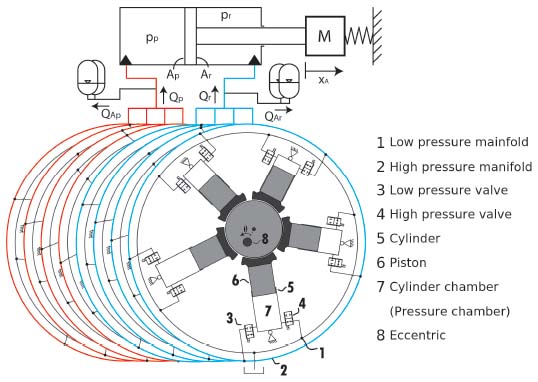
Figure 1 Conceptional drawing of a digital displacement controlled direct cylinder drive.

2.1 Dynamic Mathematical Model

A non-linear model representing the physical system is set-up to allow for simulation and performance evaluation, since a physical test-setup is not available. However, the presented model for the main cylinder has been experientially validated Schmidt et al. (2017). The cylinder motion dynamics is described by Equation (1) and is obtained by applying newtons 2nd law of motion, resulting in

$$M{\ddot{x}}_A\mathrm{<mo>=</mo>}-Kx+p_{\text{p}}{A}_{\text{p}}-p_{\text{r}}{A}_{\text{r}}-F_{\text{fric}}$$

(1)

Here M is the combined load and piston mass, while K is the spring constant. p_p and p_r is the piston and rod side pressure respectively, while A_p and A_r is the piston and rod side area respectively. The friction force, F_fric is described by a viscous and a static term given as

$$F_{\text{fric}}\mathrm{<mo>=</mo>}\underset{\text{Viscous}}{\underbrace{B_{\text{c}}{\dot{x}}_{\text{A}}}}+\underset{\text{Stribeck}\mathrm{<mi>\; </mi>}+\mathrm{<mi>\; </mi>}\text{Coloumb}}{\underbrace{\mathrm{<mo\; stretchy="false">(</mo>}{F}_{\text{c}}+\mathrm{<mo\; stretchy="false">(</mo>}{F}_{\text{s}}-F_{\text{c}}\mathrm{<mo\; stretchy="false">)</mo><mo\; stretchy="false">)</mo><mi>\; </mi>}{e}^{-\mathrm{<mo>|</mo>}\frac{{\dot{\text{x}}}_{\text{A}}}{{\text{v}}_{\text{s}}}\mathrm{<mo>|</mo>}}\tanh \mathrm{<mo\; stretchy="false">(</mo>}\text{γ}{\dot{x}}_{\text{A}}\mathrm{<mo\; stretchy="false">)</mo>}}}$$

(2)

where B_c is the viscous friction coefficient, F_c is the static Coulomb friction and F_s is the Stribeck friction coefficient. γ is a shaping factor which determines the slope of the static friction near zero velocity and v_s is a shaping factor for the Stribeck friction. The pressure in the cylinder pressure chambers are described by the continuity equation and are given by

$$\begin{array}{c}{\dot{p}}_{\text{p}}\mathrm{<mo>=</mo><mo\; stretchy="false">(</mo>}{Q}_{\text{p}}-Q_{\text{Ap}}-A_{\text{p}}{\dot{x}}_{\text{A}}\mathrm{<mo\; stretchy="false">)</mo>}\frac{{\beta }_{\text{e}}\mathrm{<mo\; stretchy="false">(</mo>}{p}_{\text{p}}\mathrm{<mo\; stretchy="false">)</mo>}}{V_{\text{p}\mathrm{,0}}+A_{\text{p}}{x}_{\text{A}}}\hfill \\ {\dot{p}}_{\text{r}}\mathrm{<mo>=</mo><mo\; stretchy="false">(</mo>}{Q}_{\text{r}}-Q_{\text{Ar}}+A_{\text{r}}{\dot{x}}_{\text{A}}\mathrm{<mo\; stretchy="false">)</mo>}\frac{{\beta }_{\text{e}}\mathrm{<mo\; stretchy="false">(</mo>}{p}_{\text{r}}\mathrm{<mo\; stretchy="false">)</mo>}}{V_{\text{r}\mathrm{,0}}-A_{\text{r}}{x}_{\text{A}}}\hfill \end{array}$$

(3)

The pressure dependent effective bulk modulus, β_e is modeled in accordance with Andersen and Hansen (2003) which includes the ratio of air entrapped in the oil and has a maximum value of β_max. V_p,init and V_r,init are the initial piston and rod side volumes respectively.

The flows into the damping accumulators are modeled as

$$\begin{array}{c}{Q}_{\text{Ap}}\mathrm{<mo>=</mo>}{K}_{\text{v}}\sqrt{\mathrm{<mo>|</mo>}{p}_{\text{p}}-p_{\text{Ap}}\mathrm{<mo>|</mo>}}\text{sgn}\mathrm{<mo\; stretchy="false">(</mo>}{p}_{\text{p}}-p_{\text{Ap}}\mathrm{<mo\; stretchy="false">)</mo>}\\ Q_{\text{Ar}}\mathrm{<mo>=</mo>}{K}_{\text{v}}\sqrt{\mathrm{<mo>|</mo>}{p}_{\text{p}}-p_{\text{Ar}}\mathrm{<mo>|</mo>}}\text{sgn}\mathrm{<mo\; stretchy="false">(</mo>}{p}_{\text{r}}-p_{\text{Ar}}\mathrm{<mo\; stretchy="false">)</mo>}\end{array}$$

(4)

where p_Ap and p_Ar are the pressures in the damping accumulators on the piston and rod side respectively. The accumulators are modeled relatively simple by considering the ideal adiabatic gas model and is given by

$$p_{\text{Ap}}\mathrm{<mo>=</mo>}{\left(\frac{V_{\text{Ap}}}{{\displaystyle \int }{Q}_{\text{Ap}}}\right)}^{\kappa }{p}_{\text{Ap}\mathrm{,0}}{p}_{\text{Ar}}\mathrm{<mo>=</mo>}{\left(\frac{V_{\text{Ar}}}{{\displaystyle \int }{Q}_{\text{Ar}}}\right)}^{\kappa }{p}_{\text{Ar}\mathrm{,0}}$$

(5)

Table 1 Parameter values used in the non-linear simulation model for the main cylinder. The cylinder model has been experimentally validated by Schmidt et al. (2017)

Parameter	Symbol	Value	Unit
Load mass	M	1316	Kg
Spring constant	K	81367	N/m
Piston side area	Ap	31.17	cm2
Rod side area	Ar	21.55	cm2
Viscous friction coefficient	Bc	6480	Ns/m
Coulomb friction	Fc	1740.8	N
Stribeck friction coefficient	Fs	1790.8	N
Stribeck velocity coefficient	vs	0.7	cm/s
Friction slope coefficient	γ	1700	–
Initial piston side volume	Vp,0	0.36	L
Initial rod side volume	Vr,0	0.54	L
Maximum oil bulk modulus	βmax	7500	bar
Accumulator size, piston	VAp	3	L
Accumulator size, rod	VAr	3	L
Adiabatic gas constant	κ	1.4	–
Pre-charge pressure, piston	pAp,0	40	bar
Pre-charge pressure, rod	pAr,0	25	bar

where κ is the adiabatic gas constant, V_Ap and V_Ar are the accumulator volumes and p_Ap,0 and p_Ar,0 are the pre-charge pressures. The parameter values of the main cylinder is provided in Table 1.

The remaining modeling governs the dynamics of the digital displacement machine, where the important characteristics with respect to control of the machine is included. The piston and rod side flows Q_p and Q_r are the sum of flows from the individual pressure chambers of the DDM given by

$$Q_{\text{p}}\mathrm{<mo>=</mo>}{\displaystyle \sum _{i\mathrm{<mo>=</mo>1}}^{{\text{N}}_{\text{c}}}}{Q}_{\text{Hp}}\mathrm{<mo\; stretchy="false">(</mo>}i\mathrm{<mo\; stretchy="false">)</mo>}{Q}_{\text{r}}\mathrm{<mo>=</mo>}{\displaystyle \sum _{i\mathrm{<mo>=</mo>1}}^{{\text{N}}_{\text{c}}}}{Q}_{\text{Hr}}\mathrm{<mo\; stretchy="false">(</mo>}i\mathrm{<mo\; stretchy="false">)</mo>}$$

(6)

where N_c = 20 is the number of cylinders. Q_Hp and Q_Hr are the flow through the high pressure valve as shown in Figure 2 illustrating a pressure chamber of the DDM. Since the dynamics of the rod side cylinder bank is identically to the piston side cylinder bank, the following derivation is made only for the piston side bank.

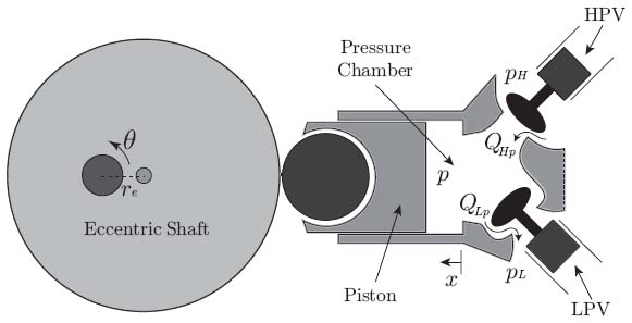
Figure 2 Illustration of a single cylinder of the radial piston digital displacement machine.

It is seen that the high pressure valve (HPV) controls the flow to and from the high pressure manifold, while the low pressure valve (LPV) controls the flow to and from the low pressure manifold, such that these in combination controls the chamber pressure. The piston stroke length, x as a function of the shaft angle is given by

$$\begin{array}{l}{x}_{\text{i}}\mathrm{<mo\; stretchy="false">(</mo>}{\theta }_{\text{i}}\mathrm{<mo\; stretchy="false">)</mo><mo>=</mo>}{r}_{\text{e}}\mathrm{<mo\; stretchy="false">(</mo>1}-\cos \mathrm{<mo\; stretchy="false">(</mo>}{\theta }_{\text{i}}\mathrm{<mo\; stretchy="false">)</mo><mo\; stretchy="false">)</mo>}\hfill \\ {\theta }_{\text{i}}\mathrm{<mo>=</mo>}\theta +\frac{2\pi }{N_{\text{c}}}\mathrm{<mo\; stretchy="false">(</mo>}i-\mathrm{1<mo\; stretchy="false">)</mo>}i\in \mathrm{<mo>\{</mo>1,}\dots \mathrm{,}{N}_{\text{c}}\mathrm{<mo>\}</mo>}\hfill \end{array}$$

(7)

r_e is the eccentric radius and is equal to half of the stroke length and N_c = 20 is the number of cylinders. The cylinder chamber volume is then described by

$$\begin{array}{l}{V}_{\text{i}}\mathrm{<mo\; stretchy="false">(</mo>}{\theta }_{\text{i}}\mathrm{<mo\; stretchy="false">)</mo><mo>=</mo>}\frac{V_{\text{d}}}{2}\mathrm{<mo\; stretchy="false">(</mo>1}-\cos \mathrm{<mo\; stretchy="false">(</mo>}{\theta }_{\text{i}}\mathrm{<mo\; stretchy="false">)</mo><mo\; stretchy="false">)</mo>}+V_0\hfill \\ \dot{V}\mathrm{<mo\; stretchy="false">(</mo>}{\theta }_{\text{i}}\mathrm{,}\dot{\theta }\mathrm{<mo\; stretchy="false">)</mo><mo>=</mo>}\frac{V_{\text{d}}}{2}\dot{\theta }\sin \mathrm{<mo\; stretchy="false">(</mo>}{\theta }_{\text{i}}\mathrm{<mo\; stretchy="false">)</mo>}\hfill \end{array}$$

(8)

where the chamber volume is given as V_d = V₀ = 2r_e A_c, with A_c being the piston area. The pressure dynamics is described by the continuity equation and is given by

$${\dot{p}}_{\text{i}}\mathrm{<mo>=</mo>}\frac{{\beta }_{\text{e}}\mathrm{<mo\; stretchy="false">(</mo>}{p}_{\text{i}}\mathrm{<mo\; stretchy="false">)</mo>}}{V_{\text{i}}}\mathrm{<mo\; stretchy="false">(</mo>}{Q}_{\text{Hp,i}}-Q_{\text{Lp,i}}-{\dot{V}}_{\text{i}}\mathrm{<mo\; stretchy="false">)</mo>}$$

(9)

where Q_Hp and Q_Lp are the flows through the high and low pressure valve respectively and β_e is the effective oil bulk modulus. The valve flows are described by the orifice equation yielding

$$\begin{array}{l}{Q}_{\text{Lp,i}}\mathrm{<mo>=</mo>}\frac{{\overline{x}}_{\text{Lp,i}}}{k_{\text{f}}}\sqrt{\mathrm{<mo>|</mo>}{p}_{\text{i}}-p_{\text{L}}\mathrm{<mo>|</mo>}}\text{sign}\mathrm{<mo\; stretchy="false">(</mo>}{p}_{\text{i}}-p_{\text{L}}\mathrm{<mo\; stretchy="false">)</mo>}\hfill \\ Q_{\text{Hp,i}}\mathrm{<mo>=</mo>}\frac{{\overline{x}}_{\text{Hp,i}}}{k_{\text{f}}}\sqrt{\mathrm{<mo>|</mo>}{p}_{\text{H}}-p_{\text{i}}\mathrm{<mo>|</mo>}}\text{sign}\mathrm{<mo\; stretchy="false">(</mo>}{p}_{\text{H}}-p_{\text{i}}\mathrm{<mo\; stretchy="false">)</mo>}\hfill \end{array}$$

(10)

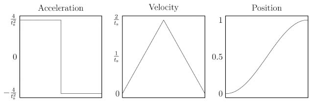
Figure 3 Dynamics response of the digital valves.

where k_f is the valve flow coefficient and ${\overline{x}}_{\text{Lp}}$ and ${\overline{x}}_{\text{Hp}}$ are normalized valve poppet positions. The poppet dynamics is modeled as a constant acceleration to yield a smooth poppet position response with a desired switching time. An illustration of the poppet dynamic response is shown in Figure 3.

Where t_s is the valve opening/closing time. The position response is similar to what may be expected if a more detailed valve model with force balance equation had been utilized. Despite the relatively simple valve model, the fundamental dynamical characteristics with respect to the behavior of the machine is included.

Valve control is achieved though active closing and passive opening due to pressure, meaning that the valves are closed at specific angles based on whether a pumping, motoring or idling decision is desired. Similarly, the HPV is opened when the chamber pressure exceeds the high pressure and the LPV is opened when the chamber pressure drops below the low pressure. Simulation results of a single chamber using the non-linear simulation model is shown in Figure 4, where all the possible activation combinations of motoring, pumping and idling is conducted.

Four different closing angles are used, namely θ_LP, θ_HP, θ_LM and θ_HM ∈ [0, 2π], which are the closing angles for the LPV during pumping, HPV during pumping, LPV during motoring and HPV during motoring respectively. Going from Section 1 to Section 2, it is seen that a pumping stroke is initiated by closing the LPV at θ_LP located at bottom dead center (BDC), which results in a pressure increase due to chamber compression. As the chamber pressure exceeds the pressure in the high pressure manifold, a passive opening of the HPV due to pressure force is achieved and high pressure fluid is pumped to the high pressure manifold. The HPV is actively closed near top dead center (TDC) at θ_HP, following a chamber decompression and a passive opening of the LPV as the chamber pressure decreases below the low pressure. Similarly, a m otoring stroke is initiated in the end of Section 4 by closing the LPV at θ_LM, resulting in a passive opening of the HPV at TDC. The HPV is further closed at θ_HM to end the motor stroke in Section 5, such that passive opening of the LPV is achieved in ahead of BDC. The later Sections 7, 8 and 9 illustrates transitions when going directly between pumping and motoring strokes. Going directly from motoring to pumping is achieved by maintaining the LPV closed and going from pumping to motoring is achieved by keeping the HPV open such that the LPV remains closed. The parameters of the digital displacement machine m odel is provided in Table 2.

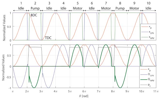
Figure 4 Simulation of a pumping, idling and motoring strokes of the digital displacement machine. The low pressure valve poppet position x_LPV and high pressure valve poppet position x_HPV indicates the activation of the valves, where a normalized position value of 1 corresponds to an open and active valve.

The reason that the maximum bulk-modulus in the DDM pressure chambers is much higher than in the main cylinder is that the hydraulic connection to the main cylinder consist of a relative large hose-volume. It is known that the pressure chamber volumes are very small in size and may be physically difficult to realize. However, the combination of chamber volume, number of pressure chambers and speed of the DDM has to be dimensioned such that they match the main cylinder specifications. With respect to control performance, it is desired to have a large number of cylinders and a high rotational speed, such that a high control resolution and update rate is achieved. However, having many small cylinder chambers is costly, why a trade off between cost and performance has to be made. Since the control strategy is the main focus of this paper and it is not effected by how these values are chosen, the above parameter values are accepted.

Table 2 Parameters of the digital displacement machine

Parameter	Symbol	Value	Unit
DDM speed	$\dot{\theta }$	1500	rpm
Piston side volume	Vd,p	1.25	cm3
Rod side volume	Vd,r	0.86	cm3
Chamber flow coefficient	kf	5 · 106	$\sqrt{pa}\mathrm{<mi>\; </mi>}\text{s}/{\text{m}}^3$
Valve actuation time	ts	3	ms
LPV motoring closing angle	θLM	337.7	deg
HPV motoring closing angle	θHM	152.2	deg
LPV pumping closing angle	θLP	179.9	deg
HPV pumping closing angle	θHP	353	deg
Low pressure	pL	1	bar
Maximum bulk-modulus	βmax	16000	bar

3 Control Strategy and DLTI Model

The mathematical model and description of the D-DHCD revealed that the dynamics of each pressure chamber is described by non-linear continuous differential equations, while the inputs (pumping, motoring or idling) are discrete and may only be updated at fixed shaft angles. To overcome these control complications, this paper proposes an angle average approximation and shows that a discrete linear time invariant (DLTI) model may be sufficient in describing the DDM dynamics. The proposed control strategy is shown in Figure 5 and is based on pulse-density modulation. Similar strategies has successfully been applied for control of both fixed and variable speed digital displacement machines which may either pump or motor, but not both Pedersen et al. (2016,2017a,b). It is seen that a multi-variable DLTI controller is utilized, which output u(t) is a displacement fraction reference for the piston and rod side DDM banks. This value is converted to an activation sequence for the DDM banks through a two-bit pulse-density modulator. A delta-sigma modulator is chosen, since its output is time averaging equal to the input due to integration of the error. The value of $\overline{u}\mathrm{<mo\; stretchy="false">(</mo>}t\mathrm{<mo\; stretchy="false">)</mo>}\in \mathrm{<mo>\{</mo>}-\mathrm{1,0,1<mo>\}</mo>}$ hence corresponds to a motoring, an idling and a pumping stroke respectively. Establishing a DLTI description of the system is seen to require a linearization of the pulse-density modulator, as well as a DLTI-approximation of the motor dynamics. Additionally, a linearization and discretization of the application load dynamics is necessary.

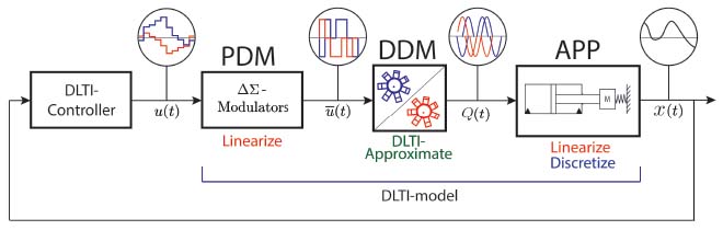
Figure 5 Illustration of the DLTI control strategy for the digital direct hydraulic cylinder drive.

3.1 Digital Displacement Machine

To obtain a synchronous sampled system, the decision to either pump, motor or idle must be synchronized. The synchronization of decisions is made by considering the flow characteristic of the DDM for the individually chambers shown in Figure 6. The fast dynamics flow spikes seen in Figure 4 caused by a rapid pressure change is omitted for simplicity of illustration.

When initiating a motoring stroke the LPV is closed at a local angle, θ_LM = ϕ_m for the specific cylinder and when initiating a pumping stroke, the LPV is closed at a local angle, θ_LP = ϕ_p for the specific cylinder. Considering two cylinders located opposite to each other, one cylinder is in the pumping stroke cycle when the other is in the motoring stroke cycle. For these opposite located cylinders, it is seen that the decision to motor is located ahead of the decision to pump. To significantly reduce the control complexity, the actuation decision for a pumping and a motor stroke is synchronized to be done at ϕ_m. The disadvantage of doing this is the minor delay introduced for pumping decisions, but since the speed of the machine is high, this time delay is very low.

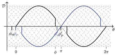
Figure 6 Two quadrant operated DDM full stroke activation pattern of two opposite located cylinders.

To develop a DLTI model of the flow characteristics, it is required that there is a linear relationship between the input and output. It is seen in Figure 6 that the response of the pumping and motoring stroke is not identically, since a minor part in the beginning of the pumping stroke is not used, while a minor part in the end of the motoring stroke is not used. However, this fraction of unused displacement is approximately identically, such that the integrated displacement during a full stroke is the same. This compliance is used in the establishment of a DLTI model where the output during a half revolution is matched. The DLTI model is established by considering the flow throughput between samples as proposed by Johansen et al. (2017). The displacement fraction between samples is described by Equation (11) when considering $Q\approx \dot{V}$, which is considered valid due to the fast pressure dynamics.

$$\begin{array}{l}{Q}_{\text{H}}\mathrm{<mo\; stretchy="false">[</mo>}k\mathrm{<mo\; stretchy="false">]</mo>}\approx \frac{V_{\text{d}}}{{\theta }_{\text{s}}}\mathrm{<mo\; stretchy="false">(</mo>}\overline{V}\mathrm{<mo\; stretchy="false">(</mo>}\theta \mathrm{<mo\; stretchy="false">[</mo>}k+\mathrm{1<mo\; stretchy="false">]</mo><mo\; stretchy="false">)</mo>}-\overline{V}\mathrm{<mo\; stretchy="false">(</mo>}\theta \mathrm{<mo\; stretchy="false">[</mo>}k\mathrm{<mo\; stretchy="false">]</mo><mo\; stretchy="false">)</mo><mo\; stretchy="false">)</mo>}\dot{\theta }\hfill \\ \approx \frac{V_{\text{d}}{N}_{\text{c}}}{2\pi }\dot{\theta }\Delta \overline{V}\mathrm{<mo\; stretchy="false">[</mo>}k\mathrm{<mo\; stretchy="false">]</mo>}\hfill \end{array}$$

(11)

where $\overline{V}$ is the normalized chamber volume and θ_s = 2π/N_c is the sample angle. The samples are made at angles given by

$$\theta \mathrm{<mo\; stretchy="false">[</mo>}k\mathrm{<mo\; stretchy="false">]</mo><mo>=</mo>}{\varphi }_{\text{m}}+\frac{2\pi }{N_{\text{c}}}\mathrm{<mo\; stretchy="false">(</mo>}k-\mathrm{1<mo\; stretchy="false">)</mo>}k\in \mathrm{<mo>\{</mo>1,}\dots \mathrm{,}{N}_{\text{c}}\mathrm{<mo>\}</mo>}$$

(12)

where ϕ_m is the local angle where the actuation decision is made. The displacement fractions between samples is determined by Equation (13) when considering a motoring stroke.

$$\Delta \overline{V}\mathrm{<mo\; stretchy="false">[</mo>}k\mathrm{<mo\; stretchy="false">]</mo><mo>=</mo>}\{\begin{array}{ll}0\hfill & \theta \mathrm{<mo\; stretchy="false">[</mo>}k\mathrm{<mo\; stretchy="false">]</mo>,}\theta \mathrm{<mo\; stretchy="false">(</mo>}k+\mathrm{1<mo\; stretchy="false">)</mo>}\notin \mathrm{<mo\; stretchy="false">[</mo>0<mo>;</mo>}\pi \mathrm{<mo\; stretchy="false">]</mo>}\hfill \\ \overline{V}\mathrm{<mo\; stretchy="false">(</mo>}\theta \mathrm{<mo\; stretchy="false">[</mo>}k+\mathrm{1<mo\; stretchy="false">]</mo><mo\; stretchy="false">)</mo>}-\overline{V}\mathrm{<mo\; stretchy="false">(</mo>}\theta \mathrm{<mo\; stretchy="false">[</mo>}k\mathrm{<mo\; stretchy="false">]</mo><mo\; stretchy="false">)</mo>}\hfill & \theta \mathrm{<mo\; stretchy="false">[</mo>}k\mathrm{<mo\; stretchy="false">]</mo>,}\theta \mathrm{<mo\; stretchy="false">(</mo>}k+\mathrm{1<mo\; stretchy="false">)</mo>}\in \mathrm{<mo\; stretchy="false">[</mo>0<mo>;</mo>}\pi \mathrm{<mo\; stretchy="false">]</mo>}\hfill \\ \overline{V}\mathrm{<mo\; stretchy="false">(</mo>}\theta \mathrm{<mo\; stretchy="false">[</mo>}k+\mathrm{1<mo\; stretchy="false">]</mo><mo\; stretchy="false">)</mo>}-\overline{V}\mathrm{<mo\; stretchy="false">(</mo>0<mo\; stretchy="false">)</mo>}\hfill & \theta \mathrm{<mo\; stretchy="false">[</mo>}k\mathrm{<mo\; stretchy="false">]</mo><mo><</mo>0<mo><</mo>}\theta \mathrm{<mo\; stretchy="false">[</mo>}k+\mathrm{1<mo\; stretchy="false">]</mo>}\hfill \\ \overline{V}\mathrm{<mo\; stretchy="false">(</mo>}\pi \mathrm{<mo\; stretchy="false">)</mo>}-\overline{V}\mathrm{<mo\; stretchy="false">(</mo>}\theta \mathrm{<mo\; stretchy="false">[</mo>}k\mathrm{<mo\; stretchy="false">]</mo><mo\; stretchy="false">)</mo>}\hfill & \theta \mathrm{<mo\; stretchy="false">[</mo>}k\mathrm{<mo\; stretchy="false">]</mo><mo><</mo>}\pi \mathrm{<mo><</mo>}\theta \mathrm{<mo\; stretchy="false">[</mo>}k+\mathrm{1<mo\; stretchy="false">]</mo>}\hfill \end{array}$$

(13)

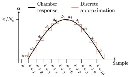
Figure 7 Discretization of displacement response.

The flow response may then be written as a convolution sum (sum of impulse responses) given by

$$Q\mathrm{<mo\; stretchy="false">[</mo>}k\mathrm{<mo\; stretchy="false">]</mo><mo>=</mo>}\underset{k_{\text{m}}}{\underbrace{\frac{V_{\text{d}}{N}_{\text{c}}\dot{\theta }}{2\pi }}}\alpha \mathrm{<mo\; stretchy="false">[</mo>}k\mathrm{<mo\; stretchy="false">]</mo>}\alpha \mathrm{<mo\; stretchy="false">[</mo>}k\mathrm{<mo\; stretchy="false">]</mo><mo>=</mo>}{\displaystyle \sum _{m\mathrm{<mo>=</mo>0}}^k}\Delta \overline{V}\mathrm{<mo\; stretchy="false">[</mo>}k-m\mathrm{<mo\; stretchy="false">]</mo>}\overline{u}\mathrm{<mo\; stretchy="false">[</mo>}m\mathrm{<mo\; stretchy="false">]</mo>}$$

(14)

where α corresponds to the displacement fraction. The resulting impulse response of the discrete displacement model is shown in Figure 7.

To match the DC-gain of the response, the committed displacement during a full stroke of the DLTI-model has to be scaled with that of the physical system where a minor fraction is not utilized. This is done by calculating the fraction of the full stroke that is utilized by

$$\eta \mathrm{<mo>=</mo>}\frac{V\mathrm{<mo\; stretchy="false">(</mo>}\varphi \mathrm{<mo\; stretchy="false">)</mo>}}{V\mathrm{<mo\; stretchy="false">(</mo>}\pi \mathrm{<mo\; stretchy="false">)</mo>}}\mathrm{<mo>=</mo>}\frac{\frac{V_{\text{d}}}{2}\mathrm{<mo\; stretchy="false">(</mo>1}-\cos \mathrm{<mo\; stretchy="false">(</mo>}\varphi \mathrm{<mo\; stretchy="false">)</mo><mo\; stretchy="false">)</mo>}}{\frac{V_{\text{d}}}{2}\mathrm{<mo\; stretchy="false">(</mo>1}-\cos \mathrm{<mo\; stretchy="false">(</mo>}\pi \mathrm{<mo\; stretchy="false">)</mo><mo\; stretchy="false">)</mo>}}\mathrm{<mo>=</mo>}\frac{\mathrm{<mo\; stretchy="false">(</mo>1}-\cos \mathrm{<mo\; stretchy="false">(</mo>}\varphi \mathrm{<mo\; stretchy="false">)</mo><mo\; stretchy="false">)</mo>}}{2}$$

(15)

where ϕ = θ_HP is the angle where motoring is stopped as shown in Figure 6. The resulting DLTI-model transfer function thus becomes that in Equation (16), when transforming the difference equation representation in Equation (14) to a transfer function.

$$G\mathrm{<mo\; stretchy="false">(</mo>}z\mathrm{<mo\; stretchy="false">)</mo><mo>=</mo>}\frac{Q}{u}\mathrm{<mo>=</mo>}\eta \mathrm{<mi>\; </mi>}{k}_{\text{m}}\frac{d_{10}{z}^{10}+d_9{z}^9+\cdots +d_{1}z+d_0}{z^{10}}$$

(16)

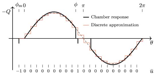
Figure 8 Two quadrant operated DDM full stroke activation pattern.

where $d_{\text{i}}\mathrm{<mo>=</mo>}\Delta \overline{V}\mathrm{<mo\; stretchy="false">[</mo>10}-i\mathrm{<mo\; stretchy="false">]</mo>}$. It is seen that the model order is directly determined by the number of cylinders. The flow response of the angle average discrete model is shown in Figure 8, for both a motoring and a pumping stroke.

The figure shows a motoring and a pumping impulse response of the DLTI-model. A value of −1 (motoring) is given as input at the first sample which output last for the subsequent 10 samples. An input value of 1 (pumping) is then given 10 samples later, which makes the same cylinder do a pumping stroke immediately after. The output is seen to resemble the system response fairly well. As expected, there are minor discrepancies in the end of the motoring stroke and in the beginning of the pumping stroke due to the linear approximation. However, the fundamental characteristics and the committed displacement during a full stroke is identical.

3.2 Pulse-density Modulator

The input $\overline{u}\in \mathrm{<mo>\{</mo>}-\mathrm{1,0,1<mo>\}</mo>}$ is generated by a discrete delta-sigma modulator that comprises of a discrete integrator and a quantizer as shown in Figure 9a.

The modulator integrates the error between the input and output such that the average value is identical. The quantizer is implemented in the form given by

$$\overline{u}\mathrm{<mo\; stretchy="false">[</mo>}k\mathrm{<mo\; stretchy="false">]</mo><mo>=</mo>}\{\begin{array}{ll}1\hfill & \text{if}v\mathrm{<mo\; stretchy="false">[</mo>}k\mathrm{<mo\; stretchy="false">]</mo>}\ge 0.5\hfill \\ 0\hfill & \text{if}-0.5\le v\mathrm{<mo\; stretchy="false">[</mo>}k\mathrm{<mo\; stretchy="false">]</mo><mo><</mo>0.5}\hfill \\ -1\hfill & \text{if}-\mathrm{0.5<mo><</mo>}v\mathrm{<mo\; stretchy="false">[</mo>}k\mathrm{<mo\; stretchy="false">]</mo>}\hfill \end{array}$$

(17)

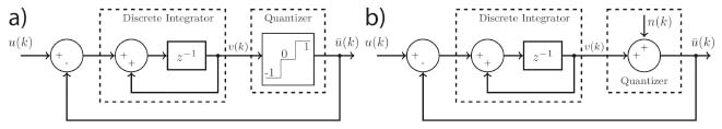
Figure 9 Two-bit first order Delta-Sigma Modulation diagram and linear representation of it.

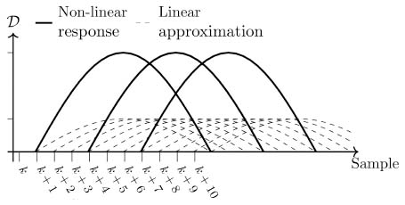
Figure 10 Comparison between linear and non-linear response.

The quantizer is seen to be highly non-linear and thus requires linearization. A typical approach to linearization of the quantizer is to split the output into a low frequency part, which contains the input signal, and a high frequency noise part. In consequence, the quantizer is modeled as an additive noise input, n with noise intensity ℐ ∈ [0; 1/2] as illustrated in Figure 9b. Replacing the quantizer with an additive noise input yields the linear discrete model given by

$$\begin{array}{l}\overline{U}\mathrm{<mo\; stretchy="false">(</mo>}z\mathrm{<mo\; stretchy="false">)</mo><mo>=</mo>}\frac{1}{z}U\mathrm{<mo\; stretchy="false">(</mo>}z\mathrm{<mo\; stretchy="false">)</mo>}+\frac{z-1}{z}N\mathrm{<mo\; stretchy="false">(</mo>}z\mathrm{<mo\; stretchy="false">)</mo>}\hfill \\ \overline{u}\mathrm{<mo\; stretchy="false">(</mo>}k\mathrm{<mo\; stretchy="false">)</mo><mo>=</mo>}u\mathrm{<mo\; stretchy="false">(</mo>}k-\mathrm{1<mo\; stretchy="false">)</mo>}+n\mathrm{<mo\; stretchy="false">(</mo>}k\mathrm{<mo\; stretchy="false">)</mo>}-n\mathrm{<mo\; stretchy="false">(</mo>}k-\mathrm{1<mo\; stretchy="false">)</mo>}\hfill \end{array}$$

(18)

It is seen that the linear model comprises of a single sample delayed input and a discrete differentiated noise term. The result of this linear approximation is illustrated by considering the relationship between the input u(k) and the output $\overline{u}\mathrm{<mo\; stretchy="false">(</mo>}k\mathrm{<mo\; stretchy="false">)</mo>}$ as shown in Figure 10. (The discretization of the response is omitted for simplicity of illustration).

It is seen that if the input u(k) = 1/3, then one third of the cylinders are activated physically. However, if neglecting the quantizer noise term, the DLTI model output results in the sum of dashed line responses. The linear response has all the cylinders active, but their amplitude is 1/3, such that the average displacement is identically. This linear approximation with neglected noise term is hence less accurate at lower displacement fractions and yields a more smooth response than the actual, which may be a limiting factor with respect to linear deterministic control of such system. The DLTI model of the modulator may then be combined with the DDM model to represent the dynamic behavior of the full stroke operated digital displacement machine.

3.3 Application Load

To apply DLTI-control of the system, the cylinder drive and load dynamics requires linearization and discretization. The mechanical system is linearized by omitting the static friction resulting in

$$M{\ddot{x}}_A\mathrm{<mo>=</mo>}-K_{\text{eq}}\mathrm{<mi>\; </mi>}x+p_{\text{p}}{A}_{\text{p}}-p_{\text{r}}\mathrm{<mi>\; </mi>}{A}_{\text{r}}-B_{\text{c}}\dot{x}$$

(19)

Linearization of the cylinder drive dynamics is done by specifying a linearization point for the effective bulk-modulus and the pressure chamber volumes, as well as neglecting the accumulator dynamics resulting in

$${\dot{p}}_p\mathrm{<mo>=</mo><mo\; stretchy="false">(</mo>}{Q}_p-A_p{\dot{x}}_A\mathrm{<mo\; stretchy="false">)</mo>}\frac{\beta }{V_p}{\dot{p}}_r\mathrm{<mo>=</mo><mo\; stretchy="false">(</mo>}{Q}_r+A_r{\dot{x}}_A\mathrm{<mo\; stretchy="false">)</mo>}\frac{\beta }{V_r}$$

(20)

The value of bulk-modulus, β, is evaluated at a relatively low pressure of 25 bar where the stiffness is low, while V_p and V_r are chosen as those yielding the lowest eigenfrequency. On state-space form the linearized system dynamics is hence described as

$$\begin{array}{c}\underset{{\dot{\mathbf{z}}}_{\text{p}}}{\underbrace{\left[\begin{array}{l}{\dot{p}}_{\text{p}}\hfill \\ {\dot{p}}_{\text{r}}\hfill \\ {\ddot{x}}_{\text{A}}\hfill \\ {\dot{x}}_{\text{A}}\hfill \end{array}\right]}}\mathrm{<mo>=</mo>}\underset{{\mathbf{A}}_{\text{c}}}{\underbrace{\left[\begin{array}{cccc}0& 0& -\frac{\beta }{V_{\text{p}}}{A}_{\text{p}}& 0\\ 0& 0& \frac{\beta }{V_{\text{r}}}{A}_{\text{r}}& 0\\ \frac{A_{\text{p}}}{M}& -\frac{A_{\text{r}}}{M}& -\frac{B_{\text{c}}}{M}& -\frac{K_{\text{ep}}}{M}\\ 0& 0& 1& 0\end{array}\right]}}\underset{{\mathbf{z}}_{\text{p}}}{\underbrace{\left[\begin{array}{l}{p}_{\text{p}}\hfill \\ p_{\text{r}}\hfill \\ {\dot{x}}_{\text{A}}\hfill \\ x_{\text{A}}\hfill \end{array}\right]}}+\underset{{\mathbf{B}}_{\text{c}}}{\underbrace{\left[\begin{array}{cc}\frac{\beta }{V_{\text{p}}}& 0\\ 0& \frac{\beta }{V_{\text{r}}}\\ 0& 0\\ 0& 0\end{array}\right]}}\underset{{\mathbf{u}}_{\text{p}}}{\underbrace{\left[\begin{array}{c}{Q}_{\text{p}}\\ Q_{\text{r}}\end{array}\right]}}\\ \underset{\mathbf{y}}{\underbrace{\left[\begin{array}{c}{x}_{\text{A}}\\ p_{\text{r}}\end{array}\right]}}\mathrm{<mo>=</mo>}\underset{{\mathbf{C}}_{\text{c}}}{\underbrace{\left[\begin{array}{cccc}0& 0& 0& 1\\ 0& 1& 0& 0\end{array}\right]}}{\mathbf{z}}_{\text{p}}\end{array}$$

(21)

The plant model is normalized to simplify control synthesis by the state transformation z_p = P x_p resulting in

$$\begin{array}{l}{\dot{\mathbf{x}}}_{\text{p}}\mathrm{<mo>=</mo>}\underset{{\mathbf{A}}_{\text{n}}}{\underbrace{{\mathbf{P}}^{-1}{\mathbf{A}}_{\text{c}}\mathbf{P}}}{\mathbf{x}}_{\text{p}}+\underset{{\mathbf{B}}_{\text{n}}}{\underbrace{{\mathbf{P}}^{-1}{\mathbf{B}}_{\text{c}}}}{\mathbf{u}}_{\text{p}}\hfill \\ \mathbf{P}\mathrm{<mo>=</mo>}\text{diag}\mathrm{<mi>\; </mi><mo\; stretchy="false">[</mo>}{\widehat{p}}_{\text{p}}{\widehat{p}}_{\text{r}}{\widehat{\dot{x}}}_{\text{A}}{\widehat{x}}_{\text{A}}\mathrm{<mo\; stretchy="false">]</mo>}\hfill \end{array}$$

(22)

where a hat denotes its maximum value. A discretization of the main cylinder plant dynamics yields the discrete state model given by

$$\begin{array}{l}{\mathbf{x}}_{\text{p}}\mathrm{<mo\; stretchy="false">(</mo>}k+\mathrm{1<mo\; stretchy="false">)</mo><mo>=</mo>}{\mathbf{A}}_{\text{p}}{\mathbf{x}}_{\text{p}}\mathrm{<mo\; stretchy="false">(</mo>}k\mathrm{<mo\; stretchy="false">)</mo>}+{\mathbf{B}}_{\text{p}}{\mathbf{u}}_{\text{p}}\mathrm{<mo\; stretchy="false">(</mo>}k\mathrm{<mo\; stretchy="false">)</mo>}\hfill \\ \mathbf{y}\mathrm{<mo\; stretchy="false">(</mo>}k\mathrm{<mo\; stretchy="false">)</mo><mo>=</mo>}{\mathbf{C}}_{\text{p}}{\mathbf{x}}_{\text{p}}\mathrm{<mo\; stretchy="false">(</mo>}k\mathrm{<mo\; stretchy="false">)</mo>}\hfill \\ {\mathbf{A}}_{\text{p}}\mathrm{<mo>=</mo>}{e}^{{\mathbf{A}}_{\text{n}}{T}_{\text{s}}}{\mathbf{B}}_{\text{p}}\mathrm{<mo>=</mo>}{\displaystyle {\int }_0^{T_{\text{s}}}}{e}^{{\mathbf{A}}_{\text{n}}\lambda }d\lambda {\mathbf{B}}_{\text{n}}{\mathbf{C}}_{\text{p}}\mathrm{<mo>=</mo>}{\mathbf{C}}_{\text{c}}\hfill \end{array}$$

(23)

The discrete transfer function of the DDM flow presented in Equation (16) may be rewritten into state space form. For the piston side flow the resulting state representation is given by

$$\begin{array}{c}\underset{{\mathbf{x}}_{\text{mp}}\mathrm{<mo\; stretchy="false">(</mo>}k+\mathrm{1<mo\; stretchy="false">)</mo>}}{\underbrace{\left[\begin{array}{c}{x}_{\text{mp}}\mathrm{<mo\; stretchy="false">(</mo>}k\mathrm{<mo\; stretchy="false">)</mo>}\\ x_{\text{mp}}\mathrm{<mo\; stretchy="false">(</mo>}k-\mathrm{1<mo\; stretchy="false">)</mo>}\\ x_{\text{mp}}\mathrm{<mo\; stretchy="false">(</mo>}k-\mathrm{2<mo\; stretchy="false">)</mo>}\\ ⋮\\ x_{\text{mp}}\mathrm{<mo\; stretchy="false">(</mo>}k-p+\mathrm{1<mo\; stretchy="false">)</mo>}\end{array}\right]}}\mathrm{<mo>=</mo>}\underset{{\mathbf{A}}_{\text{mp}}}{\underbrace{\left[\begin{array}{ccccc}0& 0& \dots & 0& 0\\ 1& 0& \dots & 0& 0\\ 0& 1& \dots & 0& 0\\ ⋮& ⋮& \ddots & ⋮& ⋮\\ 0& 0& \dots & 1& 0\end{array}\right]}}\underset{{\mathbf{x}}_{\text{mp}}\mathrm{<mo\; stretchy="false">(</mo>}k\mathrm{<mo\; stretchy="false">)</mo>}}{\underbrace{\left[\begin{array}{c}{x}_{\text{mp}}\mathrm{<mo\; stretchy="false">(</mo>}k-\mathrm{1<mo\; stretchy="false">)</mo>}\\ x_{\text{mp}}\mathrm{<mo\; stretchy="false">(</mo>}k-\mathrm{2<mo\; stretchy="false">)</mo>}\\ x_{\text{mp}}\mathrm{<mo\; stretchy="false">(</mo>}k-\mathrm{3<mo\; stretchy="false">)</mo>}\\ ⋮\\ x_{\text{mp}}\mathrm{<mo\; stretchy="false">(</mo>}k-p\mathrm{<mo\; stretchy="false">)</mo>}\end{array}\right]}}+\underset{{\mathbf{B}}_{\text{mp}}}{\underbrace{\left[\begin{array}{c}1\\ 0\\ 0\\ ⋮\\ 0\end{array}\right]}}{\overline{u}}_{\text{p}}\mathrm{<mo\; stretchy="false">(</mo>}k\mathrm{<mo\; stretchy="false">)</mo>}\\ Q_{\text{p}}\mathrm{<mo\; stretchy="false">(</mo>}k\mathrm{<mo\; stretchy="false">)</mo><mo>=</mo>}\underset{{\mathbf{C}}_{\text{mp}}}{\underbrace{k_{\text{mp}}\eta \mathrm{<mo\; stretchy="false">[</mo>}\Delta {\overline{V}}_{\text{c}}\mathrm{<mo\; stretchy="false">[</mo>1<mo\; stretchy="false">]</mo>}\cdots \Delta {\overline{V}}_{\text{c}}\mathrm{<mo\; stretchy="false">[</mo>}p\mathrm{<mo\; stretchy="false">]</mo><mo\; stretchy="false">]</mo>}}}{\mathbf{x}}_{\text{mp}}\mathrm{<mo\; stretchy="false">(</mo>}k\mathrm{<mo\; stretchy="false">)</mo>}\\ +\underset{{\mathbf{D}}_{\text{mp}}}{\underbrace{k_{\text{mp}}\eta \mathrm{<mo\; stretchy="false">[</mo>}\Delta {\overline{V}}_{\text{c}}\mathrm{<mo\; stretchy="false">[</mo>0<mo\; stretchy="false">]</mo><mo\; stretchy="false">]</mo>}}}{\overline{u}}_{\text{p}}\mathrm{<mo\; stretchy="false">(</mo>}k\mathrm{<mo\; stretchy="false">)</mo>}\end{array}$$

(24)

The only difference between the rod side and the piston side flow model of the DDM is the value of k_m, which is smaller for the rod side, since V_d is smaller to match the differential cylinder area ratio. The DLTI-model for the rod side DDM flow is thus described by

$$\begin{array}{l}{\mathbf{x}}_{\text{mr}}\mathrm{<mo\; stretchy="false">(</mo>}k+\mathrm{1<mo\; stretchy="false">)</mo><mo>=</mo>}{\mathbf{A}}_{\text{mr}}{\mathbf{x}}_{\text{mr}}\mathrm{<mo\; stretchy="false">(</mo>}k\mathrm{<mo\; stretchy="false">)</mo>}+{\mathbf{B}}_{\text{mr}}{\overline{u}}_{\text{r}}\mathrm{<mo\; stretchy="false">(</mo>}k\mathrm{<mo\; stretchy="false">)</mo>}\hfill \\ Q_{\text{r}}\mathrm{<mo\; stretchy="false">(</mo>}k\mathrm{<mo\; stretchy="false">)</mo><mo>=</mo>}{\mathbf{C}}_{\text{mr}}{\mathbf{x}}_{\text{mr}}\mathrm{<mo\; stretchy="false">(</mo>}k\mathrm{<mo\; stretchy="false">)</mo>}+D_{\text{mr}}{\overline{u}}_{\text{r}}\mathrm{<mo\; stretchy="false">(</mo>}k\mathrm{<mo\; stretchy="false">)</mo>}\hfill \end{array}$$

(25)

The flow input model to the main cylinder plant is then given as

$$\begin{array}{c}\underset{{\mathbf{x}}_{\text{m}}\mathrm{<mo\; stretchy="false">(</mo>}k+\mathrm{1<mo\; stretchy="false">)</mo>}}{\underbrace{\left[\begin{array}{c}{\mathbf{x}}_{\text{mp}}\mathrm{<mo\; stretchy="false">(</mo>}k+\mathrm{1<mo\; stretchy="false">)</mo>}\\ {\mathbf{x}}_{\text{mr}}\mathrm{<mo\; stretchy="false">(</mo>}k+\mathrm{1<mo\; stretchy="false">)</mo>}\end{array}\right]}}\mathrm{<mo>=</mo>}\underset{{\mathbf{A}}_{\text{m}}}{\underbrace{\left[\begin{array}{cc}{\mathbf{A}}_{\text{mp}}& 0\\ 0& {\mathbf{A}}_{\text{mr}}\end{array}\right]}}\underset{{\mathbf{x}}_{\text{m}}\mathrm{<mo\; stretchy="false">(</mo>}k\mathrm{<mo\; stretchy="false">)</mo>}}{\underbrace{\left[\begin{array}{c}{\mathbf{x}}_{\text{mp}}\mathrm{<mo\; stretchy="false">(</mo>}k\mathrm{<mo\; stretchy="false">)</mo>}\\ {\mathbf{x}}_{\text{mr}}\mathrm{<mo\; stretchy="false">(</mo>}k\mathrm{<mo\; stretchy="false">)</mo>}\end{array}\right]}}+\underset{{\mathbf{B}}_{\text{m}}}{\underbrace{\left[\begin{array}{cc}{\mathbf{B}}_{\text{mp}}& 0\\ 0& {\mathbf{B}}_{\text{mr}}\end{array}\right]}}\underset{\overline{\mathbf{u}}\mathrm{<mo\; stretchy="false">(</mo>}k\mathrm{<mo\; stretchy="false">)</mo>}}{\underbrace{\left[\begin{array}{c}{\overline{u}}_{\text{p}}\mathrm{<mo\; stretchy="false">(</mo>}k\mathrm{<mo\; stretchy="false">)</mo>}\\ {\overline{u}}_{\text{r}}\mathrm{<mo\; stretchy="false">(</mo>}k\mathrm{<mo\; stretchy="false">)</mo>}\end{array}\right]}}\\ \underset{{\mathbf{u}}_{\text{p}}\mathrm{<mo\; stretchy="false">(</mo>}k\mathrm{<mo\; stretchy="false">)</mo>}}{\underbrace{\left[\begin{array}{c}{Q}_{\text{p}}\mathrm{<mo\; stretchy="false">(</mo>}k\mathrm{<mo\; stretchy="false">)</mo>}\\ Q_{\text{r}}\mathrm{<mo\; stretchy="false">(</mo>}k\mathrm{<mo\; stretchy="false">)</mo>}\end{array}\right]}}\mathrm{<mo>=</mo>}\underset{{\mathbf{C}}_{\text{m}}}{\underbrace{\left[\begin{array}{cc}{\mathbf{C}}_{\text{mp}}& 0\\ 0& {\mathbf{C}}_{\text{mr}}\end{array}\right]}}\underset{{\mathbf{x}}_{\text{m}}\mathrm{<mo\; stretchy="false">(</mo>}k\mathrm{<mo\; stretchy="false">)</mo>}}{\underbrace{\left[\begin{array}{c}{\mathbf{x}}_{\text{mp}}\mathrm{<mo\; stretchy="false">(</mo>}k\mathrm{<mo\; stretchy="false">)</mo>}\\ {\mathbf{x}}_{\text{mr}}\mathrm{<mo\; stretchy="false">(</mo>}k\mathrm{<mo\; stretchy="false">)</mo>}\end{array}\right]}}+\underset{{\mathbf{D}}_{\text{m}}}{\underbrace{\left[\begin{array}{cc}{D}_{\text{mp}}& 0\\ 0& D_{\text{mr}}\end{array}\right]}}\underset{\overline{\mathbf{u}}\mathrm{<mo\; stretchy="false">(</mo>}k\mathrm{<mo\; stretchy="false">)</mo>}}{\underbrace{\left[\begin{array}{c}{\overline{u}}_{\text{p}}\mathrm{<mo\; stretchy="false">(</mo>}k\mathrm{<mo\; stretchy="false">)</mo>}\\ {\overline{u}}_{\text{r}}\mathrm{<mo\; stretchy="false">(</mo>}k\mathrm{<mo\; stretchy="false">)</mo>}\end{array}\right]}}\end{array}$$

(26)

The discrete pulse density modulator difference equation in Equation (18) is rewritten into state space form resulting in

$$\begin{array}{c}\underset{{\mathbf{x}}_{\text{d}}\mathrm{<mo\; stretchy="false">(</mo>}k+\mathrm{1<mo\; stretchy="false">)</mo>}}{\underbrace{\left[\begin{array}{c}{x}_{\text{dp}}\mathrm{<mo\; stretchy="false">(</mo>}k+\mathrm{1<mo\; stretchy="false">)</mo>}\\ x_{\text{dr}}\mathrm{<mo\; stretchy="false">(</mo>}k+\mathrm{1<mo\; stretchy="false">)</mo>}\end{array}\right]}}=\underset{{\mathbf{A}}_{\text{d}}}{\underbrace{\left[\begin{array}{cc}0& 0\\ 0& 0\end{array}\right]}}\underset{{\mathbf{x}}_{\text{d}}\mathrm{<mo\; stretchy="false">(</mo>}k\mathrm{<mo\; stretchy="false">)</mo>}}{\underbrace{\left[\begin{array}{c}{x}_{\text{dp}}\mathrm{<mo\; stretchy="false">(</mo>}k\mathrm{<mo\; stretchy="false">)</mo>}\\ x_{\text{dr}}\mathrm{<mo\; stretchy="false">(</mo>}k\mathrm{<mo\; stretchy="false">)</mo>}\end{array}\right]}}+\underset{{\mathbf{B}}_{\text{d}}}{\underbrace{\left[\begin{array}{cc}1& 0\\ 0& 1\end{array}\right]}}\underset{\mathbf{u}\mathrm{<mo\; stretchy="false">(</mo>}k\mathrm{<mo\; stretchy="false">)</mo>}}{\underbrace{\left[\begin{array}{c}{u}_{\text{p}}\mathrm{<mo\; stretchy="false">(</mo>}k\mathrm{<mo\; stretchy="false">)</mo>}\\ u_{\text{r}}\mathrm{<mo\; stretchy="false">(</mo>}k\mathrm{<mo\; stretchy="false">)</mo>}\end{array}\right]}}+\underset{{\mathbf{B}}_{\text{N}}}{\underbrace{\left[\begin{array}{cc}-1& 0\\ 0& -1\end{array}\right]}}\underset{\mathbf{n}\mathrm{<mo\; stretchy="false">(</mo>}k\mathrm{<mo\; stretchy="false">)</mo>}}{\underbrace{\left[\begin{array}{c}{n}_{\text{p}}\mathrm{<mo\; stretchy="false">(</mo>}k\mathrm{<mo\; stretchy="false">)</mo>}\\ n_{\text{r}}\mathrm{<mo\; stretchy="false">(</mo>}k\mathrm{<mo\; stretchy="false">)</mo>}\end{array}\right]}}\\ \underset{\overline{\mathbf{u}}\mathrm{<mo\; stretchy="false">(</mo>}k\mathrm{<mo\; stretchy="false">)</mo>}}{\underbrace{\left[\begin{array}{c}{\overline{u}}_{\text{p}}\mathrm{<mo\; stretchy="false">(</mo>}k\mathrm{<mo\; stretchy="false">)</mo>}\\ {\overline{u}}_{\text{r}}\mathrm{<mo\; stretchy="false">(</mo>}k\mathrm{<mo\; stretchy="false">)</mo>}\end{array}\right]}}=\underset{{\mathbf{C}}_{\text{d}}}{\underbrace{\left[\begin{array}{cc}1& 0\\ 0& 1\end{array}\right]}}\underset{{\mathbf{x}}_{\text{d}}\mathrm{<mo\; stretchy="false">(</mo>}k\mathrm{<mo\; stretchy="false">)</mo>}}{\underbrace{\left[\begin{array}{c}{x}_{\text{dp}}\mathrm{<mo\; stretchy="false">(</mo>}k\mathrm{<mo\; stretchy="false">)</mo>}\\ x_{\text{dr}}\mathrm{<mo\; stretchy="false">(</mo>}k\mathrm{<mo\; stretchy="false">)</mo>}\end{array}\right]}}+\underset{{\mathbf{D}}_{\text{N}}}{\underbrace{\left[\begin{array}{cc}1& 0\\ 0& 1\end{array}\right]}}\underset{\mathbf{n}\mathrm{<mo\; stretchy="false">(</mo>}k\mathrm{<mo\; stretchy="false">)</mo>}}{\underbrace{\left[\begin{array}{c}{n}_{\text{p}}\mathrm{<mo\; stretchy="false">(</mo>}k\mathrm{<mo\; stretchy="false">)</mo>}\\ n_{\text{r}}\mathrm{<mo\; stretchy="false">(</mo>}k\mathrm{<mo\; stretchy="false">)</mo>}\end{array}\right]}}\end{array}$$

(27)

The combined full system DLTI-model then becomes

$$\begin{array}{c}\underset{{\mathbf{x}}_{\text{t}}\mathrm{<mo\; stretchy="false">(</mo>}k+\mathrm{1<mo\; stretchy="false">)</mo>}}{\underbrace{\left[\begin{array}{c}{\mathbf{x}}_{\text{p}}\mathrm{<mo\; stretchy="false">(</mo>}k+\mathrm{1<mo\; stretchy="false">)</mo>}\\ {\mathbf{x}}_{\text{m}}\mathrm{<mo\; stretchy="false">(</mo>}k+\mathrm{1<mo\; stretchy="false">)</mo>}\\ {\mathbf{x}}_{\text{d}}\mathrm{<mo\; stretchy="false">(</mo>}k+\mathrm{1<mo\; stretchy="false">)</mo>}\end{array}\right]}}\mathrm{<mo>=</mo>}\underset{{\mathbf{A}}_{\text{t}}}{\underbrace{\left[\begin{array}{ccc}{\mathbf{A}}_{\text{p}}& {\mathbf{B}}_{\text{p}}{\mathbf{C}}_{\text{m}}& {\mathbf{B}}_{\text{p}}{\mathbf{D}}_{\text{m}}{\mathbf{C}}_{\text{d}}\\ \mathbf{0}& {\mathbf{A}}_{\text{m}}& {\mathbf{B}}_{\text{m}}{\mathbf{C}}_{\text{d}}\\ \mathbf{0}& \mathbf{0}& {\mathbf{A}}_{\text{d}}\end{array}\right]}}\underset{{\mathbf{x}}_{\text{t}}\mathrm{<mo\; stretchy="false">(</mo>}k\mathrm{<mo\; stretchy="false">)</mo>}}{\underbrace{\left[\begin{array}{c}{\mathbf{x}}_{\text{p}}\mathrm{<mo\; stretchy="false">(</mo>}k\mathrm{<mo\; stretchy="false">)</mo>}\\ {\mathbf{x}}_{\text{m}}\mathrm{<mo\; stretchy="false">(</mo>}k\mathrm{<mo\; stretchy="false">)</mo>}\\ {\mathbf{x}}_{\text{d}}\mathrm{<mo\; stretchy="false">(</mo>}k\mathrm{<mo\; stretchy="false">)</mo>}\end{array}\right]}}+\underset{{\mathbf{B}}_{\text{t}}}{\underbrace{\left[\begin{array}{c}\mathbf{0}\\ \mathbf{0}\\ {\mathbf{B}}_{\text{d}}\end{array}\right]}}\mathbf{u}\mathrm{<mo\; stretchy="false">(</mo>}k\mathrm{<mo\; stretchy="false">)</mo>}\\ +\underset{{\text{N}}_{\text{t}}}{\underbrace{\left[\begin{array}{c}{\mathbf{B}}_{\text{p}}{\mathbf{D}}_{\text{m}}{\mathbf{D}}_{\text{N}}\\ {\mathbf{B}}_{\text{m}}{\mathbf{D}}_{\text{N}}\\ {\mathbf{B}}_{\text{N}}\end{array}\right]}}\mathbf{n}\mathrm{<mo\; stretchy="false">(</mo>}k\mathrm{<mo\; stretchy="false">)</mo>}\mathbf{y}\mathrm{<mo\; stretchy="false">(</mo>}k\mathrm{<mo\; stretchy="false">)</mo><mo>=</mo>}\underset{{\mathbf{C}}_{\text{t}}}{\underbrace{\left[\begin{array}{ccc}{\mathbf{C}}_{\text{p}}& \mathbf{0}& \mathbf{0}\end{array}\right]}}{\mathbf{x}}_{\text{t}}\mathrm{<mo\; stretchy="false">(</mo>}k\mathrm{<mo\; stretchy="false">)</mo>}\end{array}$$

(28)

Since the DD unit is driven at a constant high speed $\dot{\theta }\mathrm{<mo>=</mo>1500}$ and it takes half of a revolution to go from minimum to maximum flow rate, the response time of the digital displacement machine is T_resp ≈ 0.02 s. The DDM actuation dynamics is thus relatively fast compared to the main cylinder dynamics, why it is investigated if the DDM dynamics may be neglected when synthesizing the controller. This is done through analysis of the singular values with and without the DDM dynamics. To be able to compare these values, the input to the discrete main cylinder model in Equation (23) is normalized to be given by

$${\mathbf{x}}_{\text{p}}\mathrm{<mo\; stretchy="false">(</mo>}k+\mathrm{1<mo\; stretchy="false">)</mo><mo>=</mo>}{\mathbf{A}}_{\text{p}}{\mathbf{x}}_{\text{p}}\mathrm{<mo\; stretchy="false">(</mo>}k\mathrm{<mo\; stretchy="false">)</mo>}+{\mathbf{B}}_{\text{p}}\underset{{\mathbf{u}}_{\text{p}}\mathrm{<mo\; stretchy="false">(</mo>}k\mathrm{<mo\; stretchy="false">)</mo>}}{\underbrace{{\mathbf{P}}_{\text{u}}{\mathbf{u}}_{\text{n}}\mathrm{<mo\; stretchy="false">(</mo>}k\mathrm{<mo\; stretchy="false">)</mo>}}}{\mathbf{P}}_{\text{u}}\mathrm{<mo>=</mo>}\left[\begin{array}{cc}{A}_{\text{p}}{\widehat{\dot{x}}}_{\text{A}}\eta & 0\\ 0& A_{\text{r}}{\widehat{\dot{x}}}_{\text{A}}\eta \end{array}\right]$$

(29)

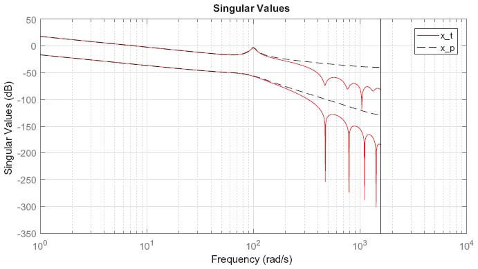
Figure 11 Comparison of singular values with and without actuator dynamics.

where P_u contains the maximum flow rate for the piston and rod side and η = 0.96 is the maximum fraction of utilized displacement. The singular values for the state equation for x_p in Equation (29) and the complete state equation x_t in Equation (28) is shown in Figure 11. It is seen that the dynamics of the DDM and modulator is so fast compared to the cylinder dynamics that the DDM dynamics may be neglected in the control design if the closed loop dynamics is slower than Ω_cl = 10 rad/s. This requirement ensures that no phase-shift is introduced to the control system by the digital machine below this frequency threshold. This requirement is easily fulfilled when designing the feedback controller. However, since the DDM states are binary (active or inactive) in reality and it is a duty-cycle ratio when analyzed linearly, neglecting the DDM dynamics might cause a reduction in performance. Therefore it is chosen to perform a simulation study of the control performance both with and without the DDM dynamics included in the control design. Also it is evident, that if the DDM is operated at a relatively low shaft speed it is always necessary to include the DDM dynamics.

4 Deterministic Optimal Control Strategy

Since the system has multiple inputs and multiple outputs, it is considered advantageous to utilize an optimal control strategy. A deterministic control strategy based on linear-quadratic regulator (LQR) is used, since it has earlier been found for a similar system, that control performance is not improved noticeable by using a stochastic method where the disturbances are included in the control design Pedersen et al. (2017a). The following section is written for control design of the full system where the DDM dynamics is included, but the same procedure it also applied for the simplified system without the DDM dynamics.

To improve set-point tracking, integral action is added to the system on the form given by

$$\begin{array}{l}{\mathbf{x}}_{\text{i}}\mathrm{<mo\; stretchy="false">(</mo>}k+\mathrm{1<mo\; stretchy="false">)</mo><mo>=</mo>}{\mathbf{x}}_{\text{i}}\mathrm{<mo\; stretchy="false">(</mo>}k\mathrm{<mo\; stretchy="false">)</mo>}+\mathbf{e}\mathrm{<mo\; stretchy="false">(</mo>}k\mathrm{<mo\; stretchy="false">)</mo>}\hfill \\ {\mathbf{x}}_{\text{i}}\mathrm{<mo\; stretchy="false">(</mo>}k+\mathrm{1<mo\; stretchy="false">)</mo><mo>=</mo>}{\mathbf{x}}_{\text{i}}\mathrm{<mo\; stretchy="false">(</mo>}k\mathrm{<mo\; stretchy="false">)</mo>}+\mathbf{r}\mathrm{<mo\; stretchy="false">(</mo>}k\mathrm{<mo\; stretchy="false">)</mo>}-{\mathbf{C}}_{\text{t}}{\mathbf{x}}_{\text{t}}\mathrm{<mo\; stretchy="false">(</mo>}k\mathrm{<mo\; stretchy="false">)</mo>}\hfill \end{array}$$

(30)

The resulting state space formulation used for control synthesis then becomes

$$\begin{array}{l}\underset{{\mathbf{x}}_{\text{s}}\mathrm{<mo\; stretchy="false">(</mo>}k+\mathrm{1<mo\; stretchy="false">)</mo>}}{\underbrace{\left[\begin{array}{c}{\mathbf{x}}_{\text{t}}\mathrm{<mo\; stretchy="false">(</mo>}k+\mathrm{1<mo\; stretchy="false">)</mo>}\\ {\mathbf{x}}_{\text{i}}\mathrm{<mo\; stretchy="false">(</mo>}k+\mathrm{1<mo\; stretchy="false">)</mo>}\end{array}\right]}}\mathrm{<mo>=</mo>}\underset{{\mathbf{A}}_{\text{s}}}{\underbrace{\left[\begin{array}{cc}{\mathbf{A}}_{\text{t}}& 0\\ -{\mathbf{C}}_{\text{t}}& \mathbf{I}\end{array}\right]}}\underset{{\mathbf{x}}_{\text{s}}\mathrm{<mo\; stretchy="false">(</mo>}k\mathrm{<mo\; stretchy="false">)</mo>}}{\underbrace{\left[\begin{array}{c}{\mathbf{x}}_{\text{t}}\mathrm{<mo\; stretchy="false">(</mo>}k\mathrm{<mo\; stretchy="false">)</mo>}\\ {\mathbf{x}}_{\text{i}}\mathrm{<mo\; stretchy="false">(</mo>}k\mathrm{<mo\; stretchy="false">)</mo>}\end{array}\right]}}+\underset{{\mathbf{B}}_{\text{s}}}{\underbrace{\left[\begin{array}{c}{\mathbf{B}}_{\text{t}}\\ \mathbf{0}\end{array}\right]}}\mathbf{u}\mathrm{<mo\; stretchy="false">(</mo>}k\mathrm{<mo\; stretchy="false">)</mo>}\hfill \\ \mathbf{y}\mathrm{<mo\; stretchy="false">(</mo>}k\mathrm{<mo\; stretchy="false">)</mo><mo>=</mo>}\underset{{\mathbf{C}}_{\text{s}}}{\underbrace{\mathrm{<mo\; stretchy="false">[</mo>}{\mathbf{C}}_{\text{t}}\mathbf{0}]}}{\mathbf{x}}_{\text{s}}\mathrm{<mo\; stretchy="false">(</mo>}k\mathrm{<mo\; stretchy="false">)</mo>}\hfill \end{array}$$

(31)

The LQR algorithm determines the optimal control input u(k) that minimizes the discrete quadratic cost function given by

$$𝒥\mathrm{<mo>=</mo>}{\displaystyle \sum _{k\mathrm{<mo>=</mo>1}}^{\infty }}\mathrm{<mo\; stretchy="false">(</mo>}{\mathbf{x}}_{\text{s}}{\mathrm{<mo\; stretchy="false">(</mo>}k\mathrm{<mo\; stretchy="false">)</mo>}}^T\mathbf{Q}{\mathbf{x}}_{\text{s}}\mathrm{<mo\; stretchy="false">(</mo>}k\mathrm{<mo\; stretchy="false">)</mo>}+\mathbf{u}{\mathrm{<mo\; stretchy="false">(</mo>}k\mathrm{<mo\; stretchy="false">)</mo>}}^{\text{T}}\mathbf{R}\mathbf{u}\mathrm{<mo\; stretchy="false">(</mo>}k\mathrm{<mo\; stretchy="false">)</mo><mo\; stretchy="false">)</mo>}$$

(32)

where Q = Q^T ≥ 0 is the state weighting matrix and R = R^T ≥ 0 is the input weighting matrix, which specifies the relative importance between driving the states to zero and the control effort to do so. It may be derived that the feedback control law is given by u(k) = −K x_t(k) + K_i x_i(k), where the feedback control gains are determined as

$${\mathbf{K}}_{\text{s}}\mathrm{<mo>=</mo><mo\; stretchy="false">(</mo>}{\mathbf{B}}_{\text{s}}^{\text{T}}{\mathbf{S\; B}}_{\text{s}}+\mathbf{R}{\mathrm{<mo\; stretchy="false">)</mo>}}^{-1}\mathrm{<mo\; stretchy="false">(</mo>}{\mathbf{B}}_{\text{s}}^{\text{T}}{\mathbf{S\; A}}_{\text{s}}\mathrm{<mo\; stretchy="false">)</mo>}$$

(33)

where the feedback gain vector is defined as K_s = [K K_i]. The unknown matrix S = S^T ≥ 0 is solved by the use of the discrete version of the algebraic Ricatti equation given by

$$\begin{array}{l}\mathbf{0}={\mathbf{A}}_{\text{s}}^{\text{T}}{\mathbf{SA}}_{\text{s}}-\mathbf{S}+\mathbf{Q}\hfill \\ -\mathrm{<mo\; stretchy="false">(</mo>}{\mathbf{A}}_{\text{s}}^{\text{T}}{\mathbf{S\; B}}_{\text{s}}\mathrm{<mo\; stretchy="false">)</mo><mo\; stretchy="false">(</mo>}{\mathbf{B}}_{\text{s}}^{\text{T}}{\mathbf{S\; B}}_{\text{s}}+\mathbf{R}{\mathrm{<mo\; stretchy="false">)</mo>}}^{-1}\mathrm{<mo\; stretchy="false">(</mo>}{\mathbf{B}}_{\text{s}}^{\text{T}}{\mathbf{S\; A}}_{\text{s}}\mathrm{<mo\; stretchy="false">)</mo>}\hfill \end{array}$$

(34)

To exemplify the control strategy presented in this paper, the state weightings are chosen in a relatively simple manner relatively to the input weighting matrix chosen as R = diag[1 1]. With reference tracking being the main objective, the integral state for the tracking error and pressure error is of high importance. Since position tracking is much more important than pressure tracking, the state weighting matrix is chosen as Q = diag {[0 0 ⋯ 5 0.001]}. With the presented method, the control synthesis has been reduced to specifying two parameters, although the system comprises of 26 states.

5 Simulation Results

Since a physical test set-up is not available and the purpose of this paper is to illustrate the potential of the concept and control strategy, only performance evaluation based on simulation results is conducted. In the simulation, a common position tracking reference has been studied and a constant pressure reference is used. Two simulations are made, one which include the digital displacement machine dynamics in the control structure and one which does not. The results of the simulation is shown in Figures 12 and 13.

The performance of the two control structures are seen to be very similar, but slightly less oscillation is identified in the piston velocity response when the complete system dynamics is included. It is clear that there is a phase-shift between the position reference and response that is undesired. This is caused by the controller gains being tuned rather conservatively. Increasing the controller gains, is found to result in an increasingly oscillating control signals and response. Minor oscillations is already seen for the piston velocity and pressure response at very low displacements, where the digital machine behavior is most clearly observed. The pressure reference tracking is also seen to be good, but as long as the pressure is within ±10 bar, the performance is considered adequate. The flow responses are actually close to what might be considered ideal, since the amplitude of the fluctuations corresponds to the actuation of a single cylinder chamber.

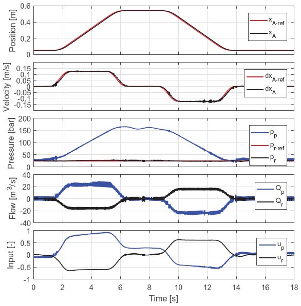
Figure 12 Without the DDM dynamics in the control structure.

Although the performance is considered acceptable it is not as good as what may be expected when using a conventional proportional valve controlled cylinder. The digital displacement technology as a direct drive is clearly most suitable for high inertia systems, where the fluctuations are dampened passively. This paper investigates a relatively low inertia system to illustrate the challenges of utilizing such digital system. Therefore, a significantly better performance is expected for high inertia systems, which control performance will be much closer to a conventional proportional valve controlled system. Alternatively, the fluctuations may be reduced by utilizing more pressure chambers with smaller volumes, but this is an expensive solution that might result in unpractical low pressure chamber volumes. Only a minor effort has been put into dimensioning of the accumulators, why optimized accumulators is also expected to increase the performance. The paper shows that the concept is viable for direct cylinder drive control, but still has many challenges that has to solved to make it a viable solution.

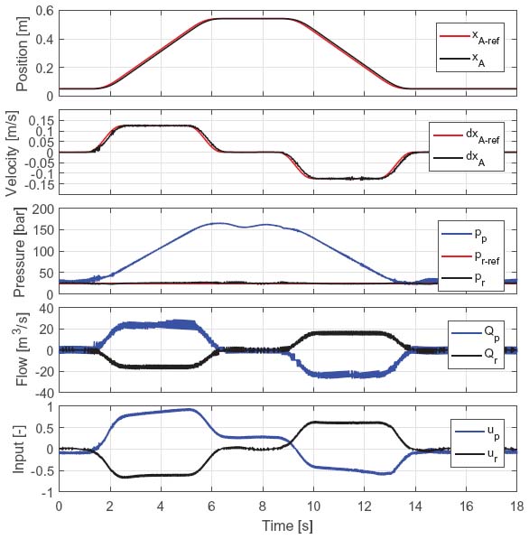
Figure 13 With the DDM dynamics in the control structure.

Conclusion

This paper proposed a control strategy for a novel energy efficient digital direct hydraulic cylinder drive concept. The highly non-smooth system behavior with both continuous and discrete dynamics challenges feedback control development. To overcome these challenges with respect to having a single machine both utilizing pumping and motoring strokes, an angle average discrete approximation of the system dynamics is established. Since the response time of the machine is proportional to its speed, a linear analysis showed that the DDM dynamics may be neglected for sufficiently high speeds. However, a simulation with the control system implemented showed that there is a slightly increase in performance by including the binary states of the digital machine in the control strategy. The system performance is found to be highly influenced by the inertia mass of the system, since a significant dampening of the digital effect is necessary to obtain smooth performance. Since this paper illustrates the concept and control system on a low mass inertia system, the obtained performance is worse than what may be expected with a conventional hydraulic cylinder drive. However, it is important to understand the digital effects, when bringing the digital displacement technology into cylinder drive systems, such that fluid power engineers know what dynamics to include in model-based design of these control systems.

Acknowledgments

This research was funded by the Danish Council for Strategic Research through the HyDrive project at Aalborg University, at the Department of Energy Technology (case no. 1305-00038B).

References

Andersen, T.O. and Hansen, M.R., 2003. Fluid Power Systems – Modelling and Analysis. 2nd edition. AAU.

Armstrong, B.S.R. and Yuan, Q., 2006. Multi-level control of hydraulic gerotor motors and pumps. Proceedings of the American Control Conference, Minnesota, USA.

Dengler, P., Geimer, M., and von Dombrowski, R., 2012. Deterministic control strategy for a hybrid hydraulic system with intermediate pressure line. Proceedings of the Fluid Power and Motion Control (FPMC), Bath, UK.

Dengler, P., Groh, J., and Geimer, M., 2011. Valve control concepts in a constant pressure system with an intermediate pressure line. 21st International Conference on Hydraulics and Pneumatics, Ostrava, Czech Republic.

Ehsan, M., Rampen, W., and Salter, S., 1997. Modeling of digital-displacement pump-motors and their application as hydraulic drives for nonuniform loads. Asme. J. Dyn. Sys., Meas., Control.

Heikkila, M. and Linjama, M., 2013. Displacement control of a mobile crane using digital hydraulic power management system. Mechatronics, volume 23, issue 4, pages 452–461.

Heybroek, K., Larsson, J., and Palmberg, J.O., 2006. Open circuit solution for pump controlled actuators. Proceedings of the 4th FPNI-PHD Symposium. Sarasota.

Heybroek, K., et al., 2008. Evaluating a pump controlled open circuit solution. Proceedings of the 51th International Exposition for Power Transmission, Nevada, USA.

Ivantysynova, M. and Rahmfeld, R., 1998. Energy saving hydraulic actuators for mobile machinery. 1st Bratislavian Fluid Power Symposium.

Johansen, P., et al., 2017. Discrete linear time invariant analysis of digital fluid power pump flow control. Journal of Dynamic Systems, Measurement and Control, Transactions of the ASME, vol. 139, no. 10, 101007.

Johansen, P., et al., 2015. Delta-sigma modulated displacement of a digital fluid power pump. The 7th Workshop on Digital Fluid Power, Linz, Austria.

Heikkilä, M. and Linjama, M. 2013. Displacement control of a mobile crane using a digital hydraulic power management system. Mechatronics, 23(4a), 452–461.

Nielsen, B., 2005. Controller Development for a Separate Meter-in Separate Meter-out Fluid Power Valve for Mobile Applications. Thesis (PhD). Department of Energy Technology, Aalborg University.

Payne, G.S., et al., 2005. Potential of digital displacement hydraulics for wave energy conversion. In Proc. of the 6th European Wave and Tidal Energy Conference, Glasgow UK.

Pedersen, N.H., Johansen, P., and Andersen, T.O., 2016. Lqr feedback control development for wind turbines featuring a digital fluid power transmission system. Proceedings of the 9th FPNI Ph.D. Symposium on Fluid Power. American Society of Mechanical Engineers.

Pedersen, N.H., Johansen, P., and Andersen, T.O., 2017a. Optimal control of a wind turbine with digital fluid power transmission. Nonlinear Dyn.

Pedersen, N.H., Johansen, P., and Andersen, T.O., 2017b. Event-driven control of a speed varying digital displacement machine. Proceedings of the 2017 BATH/ASME Symposium on Fluid Power and Motion Control.

Pedersen, N.H., Johansen, P., and Andersen, T.O., 2018. Feedback control of multi-level pulsedensity modulated digital displacement transmission. IEEE/ASME Transaction on Mecatronics, vol. x, no. x.

Rampen, W., 2010. The development of digital displacement technology. In Proceedings of BATH/ASME FPMC Symposium.

Schmidt, L., et al., 2017. Position control of an over-actuated direct hydraulic cylinder drive. Control Engineering Practice 64, 1–14.

Schmidt, L., et al., 2015. Speed-variable switched differential pump system for a direct operation of hydraulic cylinders. Proceedings of ASME/BATH Symposium on Fluid Power & Motion Control, Chicago, Illinois USA.

Sniegucki, M., Gottfried, M., and Klingauf, U., 2013. Optimal control of digital hydraulic drives using mixed-integer quadratic programming. Proceedings of the 9th IFAC Symposium on Nonlinear Control Systems.

Song, X., 2008. Modeling and active vehicle suspension system with application of digital displacement pump motor. Proceedings of the ASME 2008 International Design Engineering Technical Conferences & Computers and Information in Engineering Conference, New York, USA.

Biographies

Niels H. Pedersen received the B.Sc. and M.Sc. degrees in mechatronic control engineering from Aalborg university in 2013 and 2015, respectively. He received the Ph.D. degree also from Aalborg University in 2018 for his research and development of control strategies for digital displacement units. In 2019 he moved to R&D Engineering Solutions and Consulting A/S.

Per Johansen received the B.Sc. and M.Sc. degrees in electromechanical systems engineering and the Ph.D. degree in mechanical engineering, for his studies in tribodynamic modeling, all from the Aalborg University, Aalborg, Denmark in 2009, 2011, and 2014, respectively. Since 2014, he has been at the Department of Energy Technology, Aalborg University, where he now holds the position as Associate Professor. His main research interests include Fluid power and mechatronic systems, Tribotronics, Active tribology control methods.

Lasse Schmidt received his M.Sc. and Ph.D degrees in Mechanical Engineering from Aalborg University, Denmark, in 2008 and 2014, respectively. From 2008 to 2010 he has been with the application engineering department, Bosch Rexroth A/S, Denmark, and from 2010 to 2013 he did his Ph.D in cooperation with the same company. From 2014 to 2015 he has been a Postdoctoral Researcher at the Department of Energy Technology at Aalborg University, Denmark, concurrently being with the Engineering Application department at Bosch Rexroth AG, Lohr am Main, Germany. From 2015 to 2017 he has been an Assistant Professor at the Department of Energy Technology at Aalborg University, Denmark, and since 2017 an Associate Professor at the same department. His research interests are related to control theory as well as design and control of electro-hydraulic drives, actuators and systems. He has published research papers in international journals and conference proceedings.

Rudolf Scheidl, Born November 11th 1953 in Scheibbs (Austria). MSc of Mechanical Engineering and Doctorate of Engineering Sciences at Vienna University of Technology. Industrial research and development experience in agricultural machinery (Epple Buxbaum Werke), continuous casting technology (Voest Alpine Industrieanlagenbau), and paper mills (Voith). Since Dec. 1990 Full Professor for Mechanical Engineering at the Johannes Kepler University Linz. Research topics: hydraulic drive technology and mechatronic design.

Torben O. Andersen, since 2005 professor at the Department of Energy Technology, Aalborg University. Head of section: Fluid Power and Mecha-tronic System. Worked at Danfoss, R&D, as project manager and university coordinator. Research areas covers: control theory, energy usage and optimization of fluid power components and systems, mechatronic system in general, design and control of robotic systems and modelling and simulation of dynamic systems. Head of research programs relating development of a hydrostatic transmission for wind turbines and wave energy converters, and offshore mechatronic systems for autonomous operation and condition monitoring. Author and co-author of more than 250 scientific papers in international journals and conference proceedings.

International Journal of Fluid Power, Vol. 20_3, 295–322.
doi: 10.13052/ijfp1439-9776.2032
2020 River Publishers

Abstract

1 Introduction

2 System Description and Mathematical Model

2.1 Dynamic Mathematical Model

3 Control Strategy and DLTI Model

3.1 Digital Displacement Machine

3.2 Pulse-density Modulator

3.3 Application Load

4 Deterministic Optimal Control Strategy

5 Simulation Results

Conclusion

Acknowledgments

References

Biographies