Robust Control Design for an Inlet Metering Velocity Control System of a Linear Hydraulic Actuator
Hasan H. Ali1 and Roger C. Fales2,*
1Directorate of Reconstruction and Projects, Ministry of Higher Education and Scientific Research, Baghdad, Iraq
2Department of Mechanical and Aerospace Engineering, University of Missouri, Columbia, USA
Email: FalesR@missouri.edu
* Corresponding Author
Received 28 January 2019; Accepted 14 May 2020; Publication 23 June 2020
Abstract
In this paper, we consider a hydraulic system in which the velocity is controlled using an inlet-metered pump. The flow of the inlet-metered pump is controlled using an inlet metering valve that is placed upstream from a fixed displacement check valve pump. Placing the valve upstream from the pump reduces the energy losses across the valve. The multiplicative uncertainty associated with uncertain parameters in an inlet metering velocity control system is studied. Six parameters are considered in the uncertainty analysis. Four of the parameters are related to the valve dynamics which are the natural frequency, the damping ratio, the static gain, and the time delay. The other two parameters are the discharge coefficient and the fluid bulk modulus. Performance requirements for the system are described in the frequency domain. Frequency domain analysis is used to determine if the closed-loop velocity control system has robust performance. The time response of the nominal system with PID and H∞ controllers were found to be similar. The H∞ controller was found to have the advantages of robust performance when considering the parametric uncertainty while not requiring integral control as in the PID control system. The PID system did not achieve robust performance.
Keywords: Pump, inlet metering, velocity control, robust control.
Introduction
Background
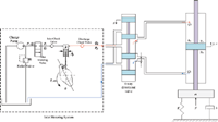
An inlet metering velocity control system is considered in this work. The inlet metering velocity control system (Figure 1) is a hydraulic system in which the velocity is controlled using an inlet-metered pump. The inlet-metered pump system is shown by the part surrounded by a dashed line in Figure 1. The flow of the inlet-metered pump is controlled using inlet metering valve that is placed upstream from a fixed displacement pump. Placing the valve upstream from the pump reduces the energy losses across the valve due to the low pressure drop across the valve when it is placed upstream from the pump. A complete description of the inlet metered pump and the inlet metering velocity control system can be found in [1] and [2]. The pump operates under the principle that inlet restriction causes a decrease in the inlet flow density by causing air to come out of solution with oil and vaporization. With a fixed displacement and constant pump speed variable flow can be achieved at the discharge due to the varying density at the inlet and inside the pump cylinder. Note that the density at the outlet does not change drastically since the discharge is assumed to be at higher pressure such that nearly all fluid will be in liquid form (no air or vapor out of solution with the hydraulic oil). Pump flow is directed to a cylinder as shown in Figure 1 with a 4-way valve that is to be used only when it is desired to change the direction of the flow.
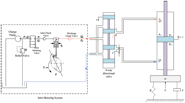
Figure 1 Inlet metering velocity control system for a linear actuator [2].
This work studies the robust stability and performance of the system under the existence of parametric uncertainty. Like any dynamic system, velocity control systems need to work under non-ideal conditions. It is important that the system stays stable and performs reasonably well when the operating conditions vary. Therefore, the control design process should consider the possible variation in the system parameters. Robust control design improves the reliability of the system by assuring that the system will be stable and have a good performance over a wide range of operating conditions and parametric uncertainty.
Literature Review
Researchers have considered the models and characteristics of various systems that include pumps with restrictions at the inlet that meter flow into the pump for various purposes. For example, Fassbender et al. [3] proposed a design of an inlet-throttled pump that reduces the amount of foam forming at the pump inlet. Foam forming has an impact on the dynamic characteristics and pumping consistency of the pump. In addition, the noise level of the pump is affected. In this design, a single valve body is used for each fluid pumping chamber. The control valve is placed at the end of the inflow channel that extends between the inlet port and the working chamber. Placing the valve in this position reduces the foam forming due to the reduction in the fluid volume. Rajput et al. [4] investigated a design of a suction-throttled multi-cylinder radial piston pump. In this study, the throttling mechanism was a rotating throttling plate that is place at the inlet port. By rotating the throttling plate, variable flow rate is achieved. Using the rotating throttling plate enhances the dynamic properties of the system since the flow of each cylinder is controlled separately which reduces the fluid volume and formation of bubbles. A study of the inlet throttling concept can also be found in [5]. In this study, a multi-piston pump is used with a throttling member at the pump inlet. The throttling member is governed by a load sensing electric actuator.An approach for controlling flow using an inlet metering valve-controlled pump for hydraulic system, which uses a fixed displacement pump to provide a variable flow, was introduced by Wisch [6]. A design of a two way inlet metering valve was given. pressure feedback and a spring were used to control the inlet metering valve so that the discharge pressure supplied to a load could be controlled. The results showed that for the special hydraulic circuit designed to control pressure using the inlet metered pump, the discharge pressure response may be approximated by a first order response. Therefore, the inlet metered pump system was found to be advantageous for use in pressure compensated circuits in which overshoot and oscillation associated with traditional pressure compensated pumps are not acceptable. The flow of the inlet-metered pump was modeled in a previous work [1].
In later work [2], a preliminary design of the velocity control system utilizing the inlet metering pump was studied. In that design, the dynamics of the inlet valve was ignored by assuming that the valve dynamics is much faster than the dynamics of the rest of the system. The stability and performance of the open-loop and the closed-loop with PD controller were studied. In another work [7], the dynamics of the valve was included. The parameters of the valve dynamics were determined experimentally. The stability and performance of the open-loop and closed-loop system with PID, H-infinity, and two degrees of freedom controllers were studied. However, the uncertainties in the systems parameters had not been considered and the robustness of the system stability and performance in the presence of uncertainty in the dynamics of the system had not been assessed.
A more complete view about the behavior of dynamic systems with uncertainty, including hydraulic systems, can be achieved by studying the perturbed system response using frequency domain analysis [8]. Coombs [9] used frequency domain analysis to study the additive and multiplicative uncertainties associated with a displacement controlled hydrostatic transmission. The uncertainty associated with a valve controlled system was studied by Fales [10]. Frequency domain was used to study the probability of the system to meet the stability and performance specifications. It was found that six percent of valve controlled systems would satisfy the performance requirements. Fales [11] designed a robust controller for a wheel loader using H-infinity loop shaping method. The multiplicative uncertainty was studied for uncertain parameters such as the fluid bulk modulus and the valve discharge coefficient.
Objectives
This paper was aimed at studying the robust stability and performance of an inlet metering velocity control system under the conditions of parametric uncertainty. Uncertainty was considered in six parameters which are, the fluid bulk modulus, the valve discharge coefficient, the valve static gain, the valve natural frequency, the valve damping ratio, and the valve time delay. Robust stability and performance of the system were analyzed in the frequency domain.
Contributions
This work is the only known effort to quantify uncertainty in the frequency domain and to determine if the feedback control stability and performance of controllers applied to the system are robust to uncertainty in parameters. The work also shows disadvantages and modest advantages of a robust H-infinity based design compared to a PID design in terms of implementation and robustness.
Outline
This work starts with a description of the velocity control system for a linear actuator using inlet metering pump system. Next, the non-dimensional governing equations of the system are given. Then, the governing equations are transformed in transfer functions. After that, a set of perturbed models is generated. From those perturbed models, the relative error (the multiplicative uncertainty) and the uncertainty weight transfer function are determined. Finally, a discussion of the results is presented and conclusions from this work are listed.
Nomenclature
| AA | Actuator Cross Sectional Area |
| Av | Opening Area of the Inlet Metering Valve |
| a | Maximum Low Frequency Error |
| b | Viscous Damping Coefficient |
| E | Error Signal |
| F | Disturbance Force |
| G | Plant Transfer Function |
| G0 | Nominal Plant Transfer Function |
| Gd | Disturbance Transfer function |
| Gp | Transfer function excluding valve dynamics |
| Gpert | Perturbed Plant Transfer Function |
| Gv | Valve Transfer Function |
| k1 | Leakage Coefficient |
| kv | Valve Static Gain |
| lI | Multiplicative Uncertainty |
| M | Maximum High Frequency Error |
| m | Mass of the Load |
| P | Generalized Plant |
| P | Pressure |
| R | Reference Signal |
| td | Valve Time Delay |
| Vo | Actuator Volume |
| v | Cylinder Velocity |
| w | Exogenous Input |
| wI | Uncertainty Weight Transfer Function |
| wP | Performance weight Transfer Function |
| wu | Controller Effort Weight Transfer Function |
| z | Exogenous Output |
| z1 | Weighted Error |
| z2 | Weighted Control Effort |
| ηa | Actuator Efficiency |
| β | Fluid Bulk Modulus |
| ωb | Bandwidth Frequency |
| ωn | Valve Natural Frequency |
| τ | Time Constant |
| ξ | Valve Damping Ratio |
| ξ1 | Non-dimensional Group |
| ξ2 | Non-dimensional Group |
| ( )A | Quantity Measured at Port A of the actuator |
| ( )b | Quantity Measured at Port B of the actuator |
| ( )d | Quantity Measured at the Pump Discharge |
| ( )i | Quantity Measured at the Valve Inlet |
| ( )r | Reference Conditions |
| (∧) | Nondimensional Quantity |
Model, Uncertainty, and Control
The governing equations of the system (excluding the inlet metering valve) are the equation of motion for the cylinder connected to a mass and spring as in Figure 1 and the pressure rise rate equation for the discharge volume of the pump which includes a cylinder chamber. These equations have been derived and nondimensionalized in a previous work [2]. The non-dimensional form of the equations is shown in Equations (1) and (2).
| (1) |
| (2) |
In Equation (2), the spring force represented by the spring stiffness, K, in Figure 1 is neglected which is typical for velocity control systems [12]. Furthermore, a linear approximation is used to model the friction force which is considered to be acceptable in the literature [12, 13]. In addition, a study of a complete hydraulic valve controlled cylinder system with Stribeckfriction and linearized reduced model of friction is presented in [14] which shows an acceptably small difference between the frequency response of the two models (non-linear full order vs. linear low order). However, in cases where the non-linear characteristics of the friction become more and more significant, the linear friction assumption would become less and less valid. And therefore, the generality of the results presented in this paper that depend on the linear friction assumption would be reduced. The details of the mathematical model can be found in [7]. The non-dimensional quantities in these two equations are defined below,
| (3) |
Then, the equations were transformed into transfer functions. Those transfer functions are the system (excluding the inlet metering valve) transfer function, Gp, the transfer function from the disturbance force to the cylinder velocity, Gd, as shown in Equation (4) and Equation (5).
| (4) |
| (5) |
The inlet metering valve dynamics transfer function was determined experimentally and it is shown in Equation (6).
| (6) |
The transfer function of the overall system dynamics, G(s), is the product of Gv(s) and Gp(s). The values of the parameters in Equations (4), (5), and (6) are given in Table A1 in the annex.
The next step is to define and model the uncertainty in the system. A set of perturbed plants is generated due to the variation of the parameters that are considered in this work over a known range. This set of plants is used to determine the relative error which is called the multiplicative uncertainty. The multiplicative uncertainty is defined as the difference between the frequency response of the perturbed and the nominal plants divided by the frequency response of the nominal plant. The multiplicative uncertainty, lI and its rational weight, wI, are given in Equation (7) and Equation (8) respectively.
| (7) |
| (8) |
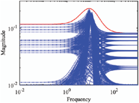
where Gpert(jω) is the perturbed plant and G0(jω) is the nominalplant. The nominal plant was found by evaluating G(jω) = Gv(s)Gp(s) with the nominal parameters which are given in Table A1. The class of perturbed plants used to generate Gpert(jω), was found by evaluating G(jω) with varying plant parameters. Six parameters are considered in the uncertainty analysis. Four of the parameters are related to the valve dynamics which are the natural frequency, the damping ratio, the static gain, and the time delay. The other two parameters are the discharge coefficient and the fluid bulk modulus. The range in which the valve dynamics parameters change is considered to be within the range of +/ − 1% of the nominal values while the change in the other two parameters are considered to be in the range of +/ − 5%. The difference in the range of the parameters variation is due to the fact that the valve dynamics parameters were determined experimentally while the discharge coefficient and the fluid bulk modulus values were only approximate. Equation (8) implies that the uncertainty weight transfer function, wI, must be greater than the maximum error, lI, for all the possible plant perturbations over all frequencies (the worst-case scenario). The upper bound on the multiplicative error in Equation (7) was found numerically by first computing the nominal plant, G(ω), and perturbations of the plant, Gpert(jω), according to a grid of the plant parameter values in the ranges given. Then the multiplicative error (the part of Equation (7) enclosed between the absolute value bars) was calculated for a range of frequencies given the nominal plant and perturbed plants (see Figure 5 presented later in the Results and Discussion section). Then the maximum value of the magnitude of the frequency responses in Figure 5 was computed according to Equation (7). To find a bounding transfer function, the uncertainty weight transfer function was found numerically by fitting a transfer function to be an approximation of the frequency response of the maximum multiplicative uncertainty (shown in Figure 5 in red). The uncertainty weight transfer function, wI, which is an upper bound on the uncertainty as in Equation (8)is given in Equation (9).
| (9) |
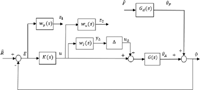
The block diagram of the system, with the performance weight, wp, the control effort weight, wu, and the multiplicative uncertainty weight, wI, transfer functions is shown in Figure 2.
Two signals z1, and z2, in Figure 2 relate to performance measures of the control system the weighed error and weighted control effort, respectively. The sensitivity transfer function is the transfer function relating the reference input, R, to the error, E, of the feedback control system in Figure 2. The performance specification of the system can be expressed in the frequency domain in terms of the desired sensitivity transfer function bandwidth, high frequency error and low frequency error levels.The performance weight that is used for performance analysis as an inverse of the upper bound on the frequency response of the sensitivity transfer function, wp, is determined using Equation (10) [15].
| (10) |
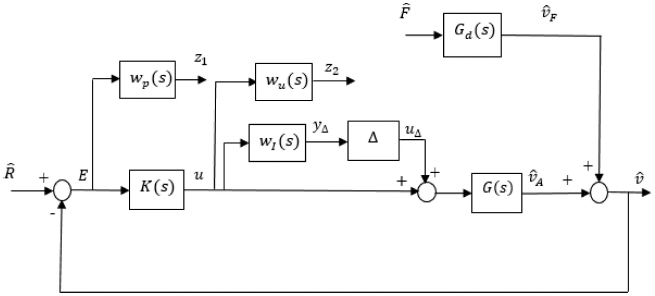
Figure 2 The system block diagram with the weights.
The non-dimensional bandwidth frequency is , the high frequency error is M = 4, and the low frequency error is a = 0.01.
The performance of the system can be further specified in terms of the control effort, u, in Figure 2. Due to the nondimensional nature of the model, it is desired to keep the control effort under one. Therefore, the control effort weight, wu, shown in Figure 2 is chosen to be one which is typical for a nondimensional system where the input is normalized about its maximum value. With the two weights chosen, the performance outputs can be analyzed given the external inputs in the frequency domain.
Two feedback controllers are considered in this paper. The PID controller was designed according to the nominal plant and auto tuning was used to determine the gains. The PID controller transfer function is . Note that the derivative term is actually zero. An H∞ control design is also considered. The controller, K(s), is obtained by finding a controller transfer function that minimizes the H∞ norm of the transfer function matrix formed from Figure 2 by relating the external inputs ( and ) to the outputs z1 and z2 while ignoring the uncertainty (letting Δ = 0). Using a standard H∞ optimization controller synthesis technique, the Matlab® function hinfsyn.m was used to produce the H∞ controller transfer function which is given in Equation (11).
| (11) |
Next, the system in Figure 2 is converted into a generalized plant transfer function which will not change the system dynamics but aid in analysis of the stability and performance using the uncertainty model and performance weights. From Figure 2, yΔ, z1, z2, and E can be written as shown in Equations (12–15).
| (12) |
| (13) |
| (14) |
| (15) |
The generalized plant, P, shown in Figure 3 can be determined as follows,
| (16) |
where w and z are the exogenous inputs and outputs respectively and are defined in Equations (17) and (18) respectively.
| (17) |
| (18) |
The P matrix consists of four elements, P11, P12, P21, and P22 as shown in Equation (19). The for elements of the P matrix are given in Equations (20–23).
| (19) |
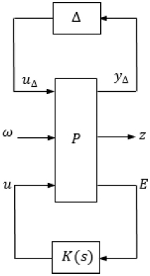
Figure 3 The general control configuration (for controller synthesis).
| (20) |
| (21) |
| (22) |
| (23) |
Substituting Equations (20–23) into Equation (19) gives the P matrix as shown in Equation (24).
| (24) |
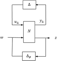
When the controller design is based on both uncertainty and performance, the structured matrix, , is considered [9]. The structured matrix is defined as shown in Equation (25).
| (25) |
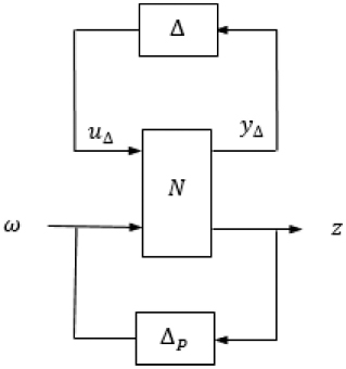
Figure 4 The N-Δ structure.
In Equation (25), △ and △P are the model and the performance uncertainties respectively. From Figure 4 and Equations (17) and (18), the model uncertainty, △, has one input, y△, and one output, u△, while the performance uncertainty, △P, has two inputs (z1 and z2) and two outputs ( and ). Also, the controller, K, has one input, E, and one output, u as shown in Figure 3. The nominal system matrix, N, is related to the generalized plant, P, and the controller, K, by a lower linear fractional transformations (LFT) given in Equation (26) [15].
| (26) |
From Figure 4, it can be noticed that N has three inputs (u△, , and ) and three outputs (y△, z1, and z2) and may be written as shown in Equation (27).
| (27) |
In order to study the system robustness, N is partitioned into four elements (N11, N12, N21, and N22) in a way similar to the way that the generalized plant P was partitioned.
Stability and performance criteria
After the N matrix had been determined, an analysis was performed to check the stability and the performance of the nominal and the perturbed system. The following are the nominal and robust stability and performance criteria that the system must meet [15].
Nominal stability (NS). The nominal stability is achieved if and only if the system, without considering the uncertainties, is stable. This means that all the poles of the nominal model are on the left half plane.
Nominal Performance (NP). The nominal performance is achieved if the system is nominally stable and satisfies the performance requirements without considering the uncertainties. This can be achieved if and only if the infinity norm (defined in [15]) of N22 is less than one as shown in Equation (28).
| (28) |
Robust Stability (RS). The system is said to be robustly stable if it remains stable for all the perturbed plants in the uncertainty set. This is achieved if and only if the infinity norm of N11 is less than one as shown in Equation (29) and the nominal system is stable.
| (29) |
Robust Performance (RP). The robust performance is achieved if the system meets the performance requirements for all the perturbed plants in the uncertainty set and it is nominally stable. For this to be true, the maximum structured singular value of N must be less than one as shown in Equation (30).
| (30) |
Results and Discussion
The multiplicative error, as in Equation (9), associated with the inlet metering velocity control system due to the variation in the design parameters over a frequency range is shown in Figure 5. It can be seen that with the current range of parameter variation, there is uncertainty of about eleven percent at low frequency, about twenty two percent at medium frequency, and about eight percent at high frequency.
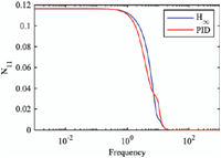
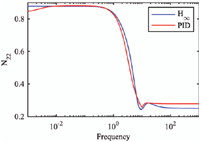
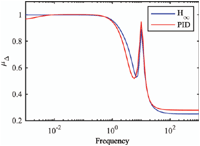
Figures 6 and 7 show that both the PID and the H∞ controllers meet the nominal stability, robust stability and the nominal performance requirements. Only the H∞ controller meets the robust performance requirement as shown in Figure 8, where μΔ is 0.995 with the H∞ controller and 1.003 with the PID controller at the peak.
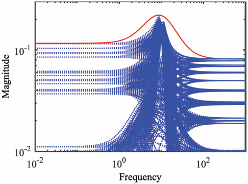
Figure 5 Multiplicative uncertainty transfer function bounding the maximum multiplicative error (Equation 7).
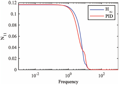
Figure 6 The robust stability requirement.
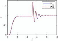
Next a simulation of the system in Figure 2 was used to demonstrate the time domain response of the nominal system without uncertainty with each of the two controllers. The simulation was completed with the following inputs, a unit step to the reference, , at zero seconds and a negative 0.75 step to the disturbance force, , at 5 seconds. Note that the simulation was accomplished by construction a block diagram as in Figure 2 in Matlab Simulink® and with the Δ block signal path in Figure 2 removed so that only the nominal system would be simulated (i.e. without uncertainty). The time response of the velocity of the nominal system with both controllers is shown in Figure 9. Both controllers give very similar nominal system time responses. There is a small disadvantage in the PID response in terms of rise time and a small amount of overshoot in the reference response seen in Figure 9 from 0 to 2 seconds. The PID controller has a small advantage in the disturbance response after 5 seconds.
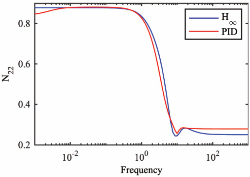
Figure 7 The nominal performance requirement.
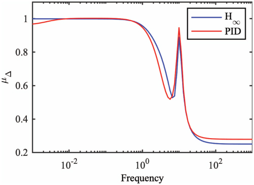
Figure 8 The robust performance requirement.
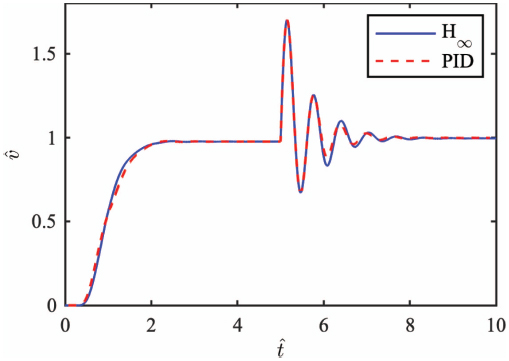
Figure 9 The time response of the system with PID and H∞ controllers.
Conclusions
The parametric uncertainty associated with an inlet metering velocity control system was studied. Stability and performance robustness to uncertainty in the dynamics of the feedback control system with PID and H∞ controllers were investigated. The time responses of the system with both controllers are essentially the same with the PID controller having a slightly better disturbance response and slightly worse reference tracking response. While both controllers meet the requirements for nominal stability, robust stability, and nominal performance, only the H∞ controller meets the robust performance requirement, although the PID controller was very close to meeting the requirement. This suggests that the complexity of the H∞ controller may not be justified. Note that the H∞ controller is sixth order, but could be reduced in order to reduce complexity. However, the PID controller implementation would likely require some additional complexity due to practical matters such as the need for measures to eliminate integrator windup. In addition to the advantage of achieving robust performance(i.e. is able to achieve stability and performance requirements even with uncertainty in the system plant dynamics), the H∞ controller has the advantage of having no pure integrator, and thus not requiring an anti-windup scheme.
This work is limited in that uncertainty due to changes in operating point are not considered directly (although these could be modeled as the parameter variations that we have included). Future work may include the investigation of non-linear control systems, motivated by the fact that the system contains nonlinearities in the pressure rise rate equation and in the equation of motion (friction nonlinearities were not considered in the model), Equation (1), which is linearized to formthe transfer functions used in analysis (Equation (4) and Equation (5)). A first step may include feedback linearization. Examples of feedback linearization and other non-linear control concepts used in fluid power literature include those discussed in [16] and the references contained therein.
Annex A
Table A1 Summarizes the values that were used in the simulations and analysis.
Table A1 Simulation values
| Parameters | Dimensional Value | Units | Non-dimensional Value |
| AA | 3.5 × 10⁻⁴ | m2 | 1 |
| Ar | 8.22 × 10⁻⁶ | m2 | 1 |
| b | 1750 | N-s/m | 0.2 |
| F | -6562.5 | N | -0.75 |
| k1 | 0.14 × 10⁻¹¹ | m4s/kg | |
| 1.21 | |||
| m | 50 | kg | 0.09 |
| Pdr | 25 × 106 | Pa | 1 |
| Pir | 2 × 10⁶ | Pa | 1 |
| td | 0.015 | s | 0.24 |
| v | 1 | m/s | 1 |
| vr | 1 | m/s | 1 |
| β | 2 × 10⁹ | Pa | |
| ωn | 85 | rad/s | 5.31 |
| τ | 0.0625 | s | |
| ξ | 0.8 | ||
| ξ1 | 10 | ||
| ξ2 | 10 |
References
[1] Ali, Hasan, J. Wisch, R. Fales, and N. Manring, “Efficiency of a Fixed Displacement Pump with Flow Control Using an Inlet Metering Valve,” ASME. J. Dyn. Sys., Meas., Control. 141(3), March 2019. doi:10.1115/1.4041606.
[2] Ali, Hasan, R. Fales, and N. Manring. “Design of a Velocity Control System Using an Inlet Metered Pump.” Bath/ASME Symposium on Fluid Power and Motion Control (FPMC 2017). Sarasota, FL. Oct. 16–19, 2017.
[3] Fassbender, A., and L. Hans-Juergen,2001, “Suction-throttled pump,” U.S. Patent No. 6,213,729.
[4] Rajput, P.K., D. Stephenson, 2015, “Hydraulic piston pump with a variable displacement throttle mechanism” U.S. Patent No. 8,926,298.
[5] Schedgick, D., B. Kramer, and J. Pfaff, 2015, “Hydraulic piston pump with throttle control” U.S. Patent No. 9,062,665.
[6] Wisch, J., “Dynamic and efficiency characteristics of an inlet metering valve controlled fixed displacement pump.” Ph.D. Dissertation, University of Missouri, 2016.
[7] Ali, H., “Inlet Metering Pump Analysis and Experimental Evaluation with Application for Flow Control,” Ph.D. Dissertation, University of Missouri-Columbia, 2017.
[8] Bax, B., P. Dean, and R. Fales, “Robust Control of a Hydraulic Metering Valve and Pump System Model” Proceedings of IMECE2006, 2006 ASME International Mechanical Engineering Congress and Exposition, November 5–10, 2006, Chicago, Illinois, USA
[9] Coombs, D., 2012, “Hydraulic Efficiency of a Hydrostatic Transmission with a Variable Displacement Pump and Motor,” M.S. Thesis, University of Missouri-Columbia.
[10] Fales, R., “Uncertainty Modeling and Predicting the Probability of Stability and Performance in the Manufacture of Dynamic Systems” ISA Transactions, 49 (2010) 528–534.
[11] Fales, R. and A. G. Kelkar, “H-Infinity Loop-Shaping Control Design and Robustness Analysis of a Hydraulic Wheel Loader” Proceedings of IMECE04, 2004 ASME International Mechanical Engineering Congress and Exposition November 13–20, 2004, Anaheim, California USA.
[12] Manring, N. D., Hydraulic Control Systems, Hoboken, NJ: John Wiley & Sons, 2005.
[13] Olesen, C., and M.Hvoldal, “Friction Modelling and Parameter Estimation for Hydraulic Asymmetrical Cylinders,” Master’s Thesis, Aalborg University, 2011.
[14] Ruderman, M., “Full- and Reduced-order Model of Hydraulic Cylinder for Motion Control,” IECON 2017 - 43rd Annual Conference of the IEEE Industrial Electronics Society, 2017, pp. 7275–7280.
[15] Skogestad, S. and I. Postlethwaite, Multivariable Feedback Control: Analysis and Design, Second Ed. New York: John Wiley and Sons, Ltd, 2005.
[16] Jelali, M., and A. Kroll, Hydraulic Servo-Systems: Modelling, Identification and Control, London: Springer-Verlag, 2003.
Biographies

Hasan H. Ali received his B.Sc. and M.Sc. degrees in Mechanical engineering from University of Tikrit, Iraq; and ME and Ph.D. degrees in Mechanical and Aerospace Engineering from University of Missouri-Columbia, USA. His research interests include modeling, design, and control of fluid power systems.

Roger C. Fales received his B.S. and M.S. degrees in Mechanical Engineering from Kansas State University; and Ph.D. in Mechanical Engineering from Iowa State University. Dr. Fales is an Associate Professor in Mechanical and Aerospace Engineering at the University of Missouri – Columbia. His research interests are in dynamics and control of fluid power systems and medical devices. He is an ASME Fellow.
International Journal of Fluid Power, Vol. 21_1, 59–80.
doi: 10.13052/ijfp1439-9776.2113
© 2020 River Publishers