Variable Speed Drive with Hydraulic Boost

Matti Linjama

Automation Technology and Mechanical Engineering Unit, Tampere University, Tampere, Finland

E-mail: matti.linjama@tuni.fi

Received 28 January 2019; Accepted 06 May 2019; Publication 17 May 2019

Abstract

This paper studies a variable speed drive with two hydraulic pump motors connected to an actuator. The torque load of the pump motors is reduced by connecting accumulators at different pressures to the inlets of the pump motors. A method for real-time selection of the inlet accumulators is developed. A linearized model is derived, and a robust control approach is used for the controller design of the variable speed drive. Simulation results indicate excellent controllability and robustness together with good energy efficiency. When three accumulators – one being a pressurized tank line – are used, the peak torque is reduced by 52 per cent compared to the traditional solution.

Keywords: Variable speed drive; hydraulics; robust control.

Introduction

Variable speed hydraulic drives (VSD) are used in modern airplanes (Mare, 2010) and also increasingly in stationary applications (Müller and Dorn, 2010). The simplest solution is to use a single pump motor to control an asymmetric cylinder (e.g. Boes and Helbig, 2014). The problem with this solution is how to compensate for the cylinder’s asymmetry.An alternative approach is to use two pump motors, one for each cylinder chamber (Minav et al., 2014). Promising results have been achieved in terms of energy efficiency (Zhang et al., 2017), but controllability has been a problem (Filatov et al., 2018). The main obstacle to the wider application of VSD technology is the high cost of the electric servomotor and inverter. This has limited the technology mainly to low-power applications. The situation is especially severe in lifting type actuation, where a large actuator force is constantly needed. This requires continuously large torque from the electric motor, which results in large electric components and increased losses.

Attempts have been made to reduce the torque needed from the electric motor. Koitto et al. (2018) suggested using a balancing cylinder to compensate for the gravitational load, but this solution requires nearly constant load forces and an extra cylinder. Tikkanen and Tommila (2015) used an extra accumulator and achieved a 25 per cent reduction in the torque. Linjama et al. (2015) also presented a solution based on a hydraulic accumulator, but the solution was not analysed further in the paper. They called this kind of solution a ‘hybrid actuator’, because two energy sources – hydraulic and electric – were used.

This paper studies a VSD with a novel load-balancing solution in which the balancing torque is created by several hydraulic accumulators. The solution works with varying loads and significantly reduces the torque and power needed from the electric servomotor. The hydraulic circuit diagram of the solution is shown in Figure 1. The system has N accumulators at different pressures and a VSD with two pump motors. Accumulators are charged by a tiny on/off pump (referred to in this paper as a bilge pump) when needed. The first accumulator is a pressurized tank, and no zero-pressure tank is used. This requires the replacement of the shaft seals of the pump motors and the bilge pump (Paloniitty et al., 2018). The target of this paper is to answer the following questions:

1. How large transients occur when inlet pressures of the pump motors change stepwise?
2. How many accumulators are needed in order to significantly reduce the peak torque and power of the electric servomotor?
3. Is it possible to improve controllability of the VSD drives by a robust control approach?

Simulations are used to find the answers to these questions. The verified simulation model of the electric servomotor is used, and a simple leakage model is included in the pump model in order to study the effect of leakages on performance. A linearized model is derived, and a robust controller is designed for the system. Simulation results show a combination of excellent controllability and robustness as well as good energy efficiency, but at least three accumulators are needed. One accumulator (tank pressure only) yields a large peak torque, and the two-accumulator solution (tank plus high pressure) has large switching transients. The peak torque is reduced by 52 per cent when three accumulators are used. The simulation results also show that relatively small accumulators are sufficient.

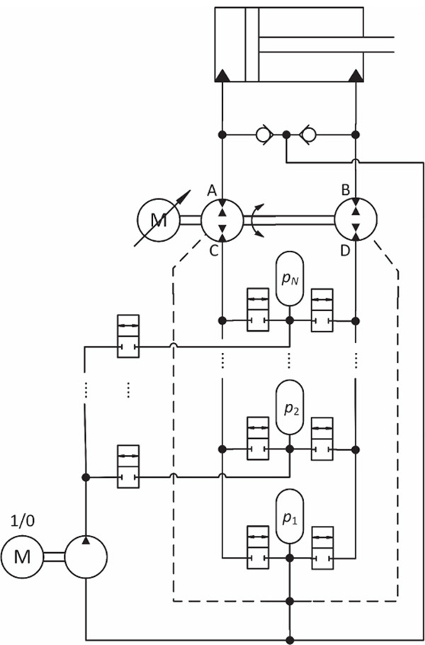
Figure 1 Hydraulic circuit diagram of the approach studied in this paper.

System Model

Electric Servomotor and Inverter

The electric servomotor is a permanent magnet synchronous motor running in field-oriented control mode. Its modelling principles are well known (Belda 2013). The assumptions here are:

1. The electromagnetic forces are sinusoidal;
2. Surface mounted permanent magnets are used and the inductances L_d and L_q are thus equal constants, marked as L_S ;
3. Saturation of the electrical quantities is not considered;
4. The inverter is otherwise ideal, but an additional first order lag and delay are included for more realistic results;
5. The maximum rate of the target value of the rotational speed is limited.

The modelling is built on the rotor’s direct and quadrature (d-q) axis. The currents on the direct and quadrature axis (i_d and i_q, respectively) are solved from the following differential equation:

$$\frac{d}{dt}\left[\begin{array}{c}{i}_d\\ i_q\end{array}\right]=\left[\begin{array}{cc}-<!--\; -\; -->\frac{R_S}{L_S}& {\mathrm{\omega <!--\; ?\; -->}}_S\\ -<!--\; -\; -->{\mathrm{\omega <!--\; ?\; -->}}_S& -<!--\; -\; -->\frac{R_S}{L_S}\end{array}\right]\left[\begin{array}{l}{i}_d\\ i_q\end{array}\right]+\left[\begin{array}{c}\frac{u_d}{L_S}\\ \frac{u_q-<!--\; -\; -->{\mathrm{\omega <!--\; ?\; -->}}_S{\mathrm{\psi <!--\; ?\; -->}}_{pm}}{L_S}\end{array}\right](1)$$

where Rs is the stator line-to-neutral resistance, L_S is the inductance on the d-q axis (L_S = L_d = L_q ) and ω_S is the electrical rotational speed of the rotor. The electrical and mechanical rotational speeds are related by:

$${\mathrm{\omega <!--\; ?\; -->}}_S=P\mathrm{\omega <!--\; ?\; -->}(2)$$

where P is the number of pole pairs and ω is the mechanical rotational speed. ψ_pm is the flux linkage of the permanent magnets which is given by:

$${\mathrm{\psi <!--\; ?\; -->}}_{pm}=\frac{2K_t}{3P}(3)$$

where K_t is the torque constant of the motor. The torque is controlled by i_q and the controller tries to keep i_d at zero. It is assumed that the currents are controlled by PI-controllers:

$$\begin{array}{l}{u}_d=-<!--\; -\; -->K_{P,d}{i}_d-<!--\; -\; -->K_{I,d}\int <!--\; ?\; -->i_{d}dt\\ u_q=K_{P,q}(i_{q,ref}-<!--\; -\; -->i_q)+K_{I,q}\int <!--\; ?\; -->i_{q,ref}-<!--\; -\; -->i_{q}dt\end{array}(4)$$

The velocity controller is also assumed to be PI-controller:

$$i_{q,ref}=K_{P,n}({\mathrm{\omega <!--\; ?\; -->}}_{ref}-<!--\; -\; -->\mathrm{\omega <!--\; ?\; -->})+K_{I,n}\int <!--\; ?\; -->{\mathrm{\omega <!--\; ?\; -->}}_{ref}-<!--\; -\; -->\mathrm{\omega <!--\; ?\; -->}dt(5)$$

The electromagnetic torque produced by the motor is

$${\mathrm{\tau <!--\; t\; -->}}_M=K_t{i}_q-<!--\; -\; -->b_{\mathrm{\tau <!--\; t\; -->},pm}\mathrm{\omega <!--\; ?\; -->}(6)$$

where b_τ,pm is the viscous friction coefficient. The torque balance equation is:

$$(J_M+J_{PM})\stackrel{\dot{}<!--\; ?\; -->}{\mathrm{\omega <!--\; ?\; -->}}={\mathrm{\tau <!--\; t\; -->}}_M-<!--\; -\; -->{\mathrm{\tau <!--\; t\; -->}}_{PM}(7)$$

where J_M and J_PM are the moments of inertia of the electric servomotor and pump motors, respectively, and τ PM is the torque needed to rotate the pump motors.

The electric servomotor used is a Parker GVM142-050-MPW with an MCD-04-0450 inverter driven by a 48 VDC battery (Anon, 2017). The parameters of the electric servomotor and inverter are shown in Table 1. They are from the manufacturer’s catalogue except the input delay, inverter time constant and parameters of the current and speed controllers, which are tuned so that the measured and simulated responses match.

The electric servomotor model is validated using the hydraulic loading system described by Leinamo (2018). The load is a 10.6 cc pump-motor and the loading system is able to create different pressure differentials over the pump-motor. Figure 2 presents the measured and simulated speed step responses when the pressure differential is around 0.5 MPa. The modelling accuracy is good and the delay is significant at around 30 ms. Figure 3 shows the measured and simulated responses when the load pressure experiences stepwise changes; the measured response has more oscillations but the modelling accuracy is otherwise good. The peak error in rotational speed is quite large.

Table 1 Parameters of the electric servomotor and inverter

Rotor inertia (JM)	0.0021 kg m2
Input delay	30 ms
Rated power	3.22 (7.94*) kW
Rated/max torque	7.7 (18.1*) / 40.0 Nm
Rated/max speed	4200 / 6300 r/min
Rated/max current	74.4 (175*) / 450 Arms
Number of pole pairs (P)	6
Stator phase resistance, phase to phase (RS)	6.94 mω
Stator inductance, phase to phase (LS)	0.0453 mH
Torque constant (Kt)	0.104 Nm/Arms
Inverter electric time constant	15 ms
Maximum rate of the target speed	2500 rad/s2
Speed controller proportional gain (KP,n)	2.5 A/(rad/s)
Speed controller integral gain (KI,n)	15As–1/(rad/s)
Current controller proportional gain, d-axis (KP,d)	2 V/A
Current controller proportional gain, q-axis (KP,q)	0 V/A
Current controller integral gain, d-axis (KI,d)	0 V/(A s)
Current controller integral gain, q-axis (KI,q)	2.5 V/(A s)
Viscous friction coefficient (bτ,pm)	0.001 Nm/(rad/s)

*Value with liquid cooling

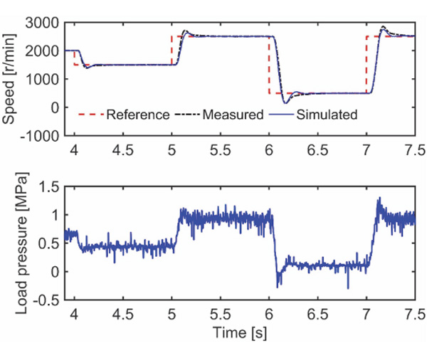
Figure 2 Measured and simulated velocity step responses with small load torque.

Pump Motors

The port names and positive flow directions of the pump motors are shown in Figure 4. Ports A and B are the ‘actuator side’ and ports C and D the ‘supply side’ of the pump motors. The pump motors are modelled as follows:

$$\begin{array}{rl}{Q}_{PM,A}& =V_{rad1}\mathrm{\omega <!--\; ?\; -->}-<!--\; -\; -->V_{rad1}{K}_L(p_A-<!--\; -\; -->p_C)-<!--\; -\; -->V_{rad1}{K}_L(p_A-<!--\; -\; -->p_1)\\ Q_{PM,B}& =-<!--\; -\; -->V_{rad2}\mathrm{\omega <!--\; ?\; -->}-<!--\; -\; -->V_{rad2}{K}_L(p_B-<!--\; -\; -->p_D)-<!--\; -\; -->V_{rad2}{K}_L(p_B-<!--\; -\; -->p_1)\\ Q_{PM,C}& =-<!--\; -\; -->V_{rad1}\mathrm{\omega <!--\; ?\; -->}+V_{rad1}{K}_L(p_A-<!--\; -\; -->p_C)-<!--\; -\; -->V_{rad1}{K}_L(p_C-<!--\; -\; -->p_1)\\ Q_{PM,D}& =V_{rad2}\mathrm{\omega <!--\; ?\; -->}+V_{rad2}{K}_L(p_B-<!--\; -\; -->p_D)-<!--\; -\; -->V_{rad2}{K}_L(p_D-<!--\; -\; -->p_1)\\ Q_{L1}& =V_{rad1}{K}_L(p_A-<!--\; -\; -->p_1)+V_{rad1}{K}_L(p_C-<!--\; -\; -->p_1)\\ Q_{L2}& =V_{rad2}{K}_L(p_B-<!--\; -\; -->p_1)+V_{rad2}{K}_L(p_D-<!--\; -\; -->p_1)\\ {\mathrm{\tau <!--\; t\; -->}}_{PM}& =V_{rad1}(p_A-<!--\; -\; -->p_C)-<!--\; -\; -->V_{rad2}(p_B-<!--\; -\; -->p_D)+{\mathrm{\tau <!--\; t\; -->}}_{\mathrm{\mu <!--\; \mu \; -->}1}+{\mathrm{\tau <!--\; t\; -->}}_{\mathrm{\mu <!--\; \mu \; -->}2}\end{array}(8)$$

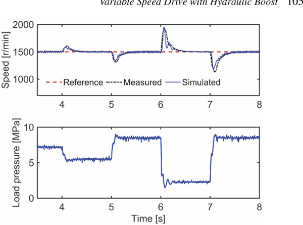
Figure 3 Measured and simulated rotational speeds with torque disturbances.

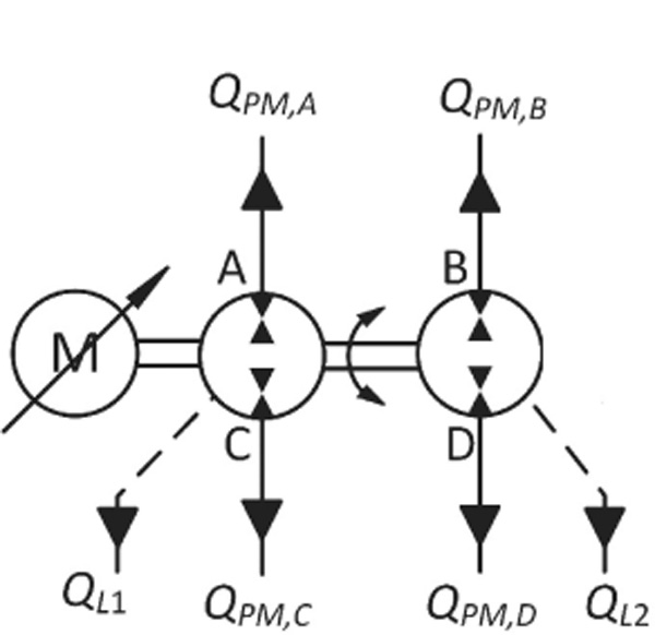
Figure 4 Flow definitions for the pump motors.

where V_rad1 and V_rad2 are the radian displacements of the A-side and B-side pump motors, respectively, and p_A, p_B, p_C and p_D are pressures at ports A, B, C and D, respectively. The leakage flows are assumed to be proportional to the radian displacement and pressure differential. The laminar flow coefficient K_L is assumed to be the same for all leakage paths. It is clear that the model is not accurate, but it is important to have some kind of leakage model in order to avoid unrealistic results. The friction torque model is adopted from Huova et al. (2018):

$$\begin{array}{l}{\mathrm{\tau <!--\; t\; -->}}_{\mathrm{\mu <!--\; \mu \; -->}1}=V_{rad1}\tanh <!--\; ?\; -->(20\cdot <!--\; ·\; -->\mathrm{\omega <!--\; ?\; -->})\\ \text{enskip}(8.4\times <!--\; \times \; -->{10}^5+0.020\cdot <!--\; ·\; -->|p_A-<!--\; -\; -->p_C|+200\cdot <!--\; ·\; -->\left|\mathrm{\omega <!--\; ?\; -->}\right|+0.11\cdot <!--\; ·\; -->{\mathrm{\omega <!--\; ?\; -->}}^2)\\ {\mathrm{\tau <!--\; t\; -->}}_{\mathrm{\mu <!--\; \mu \; -->}2}=V_{rad2}\tanh <!--\; ?\; -->(20\cdot <!--\; ·\; -->\mathrm{\omega <!--\; ?\; -->})\\ \text{enskip}(8.4\times <!--\; \times \; -->{10}^5+0.020\cdot <!--\; ·\; -->|p_B-<!--\; -\; -->p_D|+200\cdot <!--\; ·\; -->\left|\mathrm{\omega <!--\; ?\; -->}\right|+0.11\cdot <!--\; ·\; -->{\mathrm{\omega <!--\; ?\; -->}}^2)\end{array}(9)$$

Figure 5 shows the efficiency curves with the parameters used in this study. The unit runs as a pump with zero inlet pressure, and the rotational speed is 1500 r min^–1. The volumetric efficiency for the zero inlet pressure is:

$${\mathrm{\eta <!--\; ?\; -->}}_{vol}=1-<!--\; -\; -->\frac{2V_{rad}{K}_L\mathrm{\Delta <!--\; ?\; -->}p}{V_{rad}\mathrm{\omega <!--\; ?\; -->}}=1-<!--\; -\; -->\frac{2K_L\mathrm{\Delta <!--\; ?\; -->}p}{\mathrm{\omega <!--\; ?\; -->}}(10)$$

The mechanical efficiency is calculated in view of Equation 9 as follows:

$${\mathrm{\eta <!--\; ?\; -->}}_{mh}=1-<!--\; -\; -->\frac{8.4\times <!--\; \times \; -->{10}^5+0.020\cdot <!--\; ·\; -->\mathrm{\Delta <!--\; ?\; -->}p+200\cdot <!--\; ·\; -->\mathrm{\omega <!--\; ?\; -->}+0.11\cdot <!--\; ·\; -->{\mathrm{\omega <!--\; ?\; -->}}^2}{\mathrm{\Delta <!--\; ?\; -->}p}(11)$$

The total efficiency is obtained as a product of volumetric and mechanical efficiency.

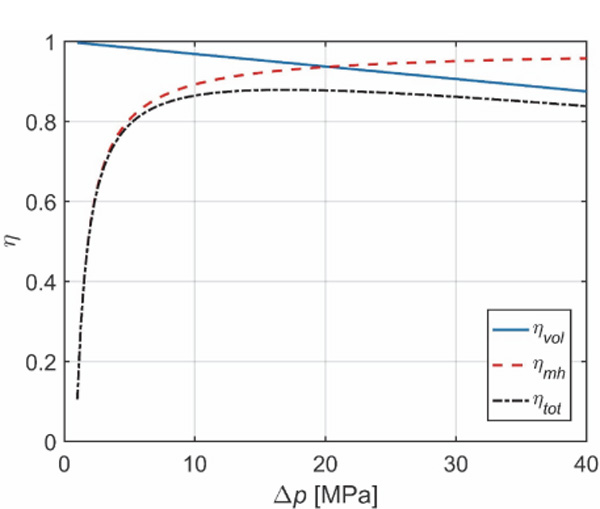
Figure 5 Efficiency curves when suction pressure is zero and the rotational speed is 1500 r min^–1.

Accumulators, on/off Valves and Bilge Pump

The accumulator module of Figure 6 is modelled using the standard pressure build-up equation, square root flow model and ideal gas equation:

$$\begin{array}{r}\begin{array}{rcl}{\stackrel{\dot{}<!--\; ?\; -->}{p}}_i& =& \frac{B}{V_i}(Q_{bilge}-<!--\; -\; -->Q_{i,C}-<!--\; -\; -->Q_{i,D}-<!--\; -\; -->Q_{i,acc})\\ Q_{i,C}& =& K_{v,valve}{x}_{i,C}\left(u_{i,C}\right)sgn(p_i-<!--\; -\; -->p_C)\sqrt{|p_i-<!--\; -\; -->p_C|}\\ Q_{i,D}& =& K_{v,valve}{x}_{i,D}\left(u_{i,D}\right)sgn(p_i-<!--\; -\; -->p_D)\sqrt{|p_i-<!--\; -\; -->p_D|}\\ Q_{i,acc}& =& K_{v,acc}sgn(p_i-<!--\; -\; -->p_{acc})\sqrt{|p_i-<!--\; -\; -->p_{i,acc}|}\\ p_{i,acc}& =& {\left(\frac{V_{0,i}}{\int <!--\; ?\; -->Q_{i,acc}dt}\right)}^{1.4}{p}_{0,i}\end{array}\end{array}(12)$$

where B is the bulk modulus, V_i is the size of the volume between valves, and Q_bilge is the flow rate from the bilge pump into the volume. K_v,valve is the flow coefficient of the control valves, x_i,C and x_i,D are relative openings of the control valves, u_i,C and u_i,D are control signals of the control valves, K_v,acc is the flow coefficient of the port orifice of the accumulator, V_0,i is the volume of the accumulator and p_0,i is the pre-charge pressure of the accumulator. The equa-tions for the lowest pressure are similar, but the pressure build-up equation is:

$${\stackrel{\dot{}<!--\; ?\; -->}{p}}_1=\frac{B}{V_1}(Q_{L1}+Q_{L2}-<!--\; -\; -->Q_{bilge}-<!--\; -\; -->Q_{1,C}-<!--\; -\; -->Q_{1,D}-<!--\; -\; -->Q_{1,acc})(13)$$

The dynamics of the on/off valves is modelled with delay plus constant opening and closing rate. The bilge pump is modelled as an ideal on/off flow source.

Figure 6 Flow definitions for the accumulator module.

It takes the flow from the lowest pressure and pumps it into one of the higher pressures.

Volumes between Valves and Pump Motors

The pressure build-up equations for the volumes between valves and pump motors are:

$$\begin{array}{l}{\stackrel{\dot{}<!--\; ?\; -->}{p}}_C=\frac{B}{V_C}(\underset{i=1}{\overset{N}{\sum <!--\; ?\; -->}}{Q}_{i,C}+Q_{PM,C})\\ {\stackrel{\dot{}<!--\; ?\; -->}{p}}_D=\frac{B}{V_D}(\underset{i=1}{\overset{N}{\sum <!--\; ?\; -->}}{Q}_{i,D}+Q_{PM,D})\end{array}(14)$$

where V_C and V_D are the sizes of volumes C and D, respectively.

Cylinder Actuator and Check Valves

The pressure build-up equations for the cylinder chambers are:

$$\begin{array}{l}{\stackrel{\dot{}<!--\; ?\; -->}{p}}_A=\frac{B_A}{A_{A}x+V_{0A}}(Q_{PM,A}+Q_{check,A}-<!--\; -\; -->A_A\stackrel{\dot{}<!--\; ?\; -->}{x})\\ {\stackrel{\dot{}<!--\; ?\; -->}{p}}_B=\frac{B_B}{A_B(x_{max}-<!--\; -\; -->x)+V_{0B}}(Q_{PM,B}+Q_{check,B}+A_B\stackrel{\dot{}<!--\; ?\; -->}{x})\end{array}(15)$$

where A_A and A_B are piston areas, V_0A and V_0B are A- and B-side dead volumes, x is the piston position, x˙ is the piston velocity and xmax is the piston stroke. The first order dynamics is assumed for the check valve and the flow rate of the A-side check valve is modelled as follows:

$$\begin{array}{r}\begin{array}{rcl}{\stackrel{\dot{}<!--\; ?\; -->}{y}}_A& =& \frac{1}{{\mathrm{\tau <!--\; t\; -->}}_{check}}(\frac{1}{\mathrm{\Delta <!--\; ?\; -->}{p}_{open}}(p_1-<!--\; -\; -->p_A)-<!--\; -\; -->y_A)\\ y_A& =& \int <!--\; ?\; -->{\stackrel{\dot{}<!--\; ?\; -->}{y}}_{A}dt,y_A\in <!--\; ?\; -->\{0\dots <!--\; \dots \; -->1\}\\ Q_{check,A}& =& K_{v,check}{y}_{A}sgn(p_1-<!--\; -\; -->p_A)\sqrt{|p_1-<!--\; -\; -->p_A|}\end{array}\end{array}(16)$$

where y_A is the relative opening of the valve, τ_check is the time constant, Δp_open is the pressure differential at which the check valve is fully open and K_v,check is the flow coefficient of the check valve. The equations for the B-side check valve are similar. The force balance equation of the cylinder actuator is:

$$m\stackrel{¨<!--\; ¨\; -->}{x}=p_A{A}_A-<!--\; -\; -->p_B{A}_B-<!--\; -\; -->F_{load}-<!--\; -\; -->F_{\mathrm{\mu <!--\; \mu \; -->}}(17)$$

where F_load is the load force, and the friction force F_μ is modelled using the dynamic friction model (Canudas de Wit et al., 1995):

$$\begin{array}{l}\stackrel{\dot{}<!--\; ?\; -->}{z}=\stackrel{\dot{}<!--\; ?\; -->}{x}-<!--\; -\; -->\frac{{\mathrm{\sigma <!--\; s\; -->}}_0\left|\stackrel{\dot{}<!--\; ?\; -->}{x}\right|}{F_C+(F_S-<!--\; -\; -->F_C)e^{-<!--\; -\; -->{\left(\stackrel{\dot{}<!--\; ?\; -->}{x}/v_s\right)}^2}}z\\ F_{\mathrm{\mu <!--\; \mu \; -->}}\left(\stackrel{\dot{}<!--\; ?\; -->}{x}\right)={\mathrm{\sigma <!--\; s\; -->}}_{0}z+{\mathrm{\sigma <!--\; s\; -->}}_1\stackrel{\dot{}<!--\; ?\; -->}{z}+b\stackrel{\dot{}<!--\; ?\; -->}{x}\end{array}(18)$$

The state variable z is the seal deflection, F_S is the static friction force, F_C is the Coulomb friction force, b is the viscous friction coefficient and v_S is related to the velocity of the minimum friction force. The parameter ς₀ is the stiffness and ς₁ the damping coefficient of the seal.

Controller Design

Linearized Model of the System

The continuous time linearized model is created under the following assumptions:

1. Dynamics of the inverter and electric servomotor is modelled as pure delay.
2. Sampling is modelled as a delay of half the sampling period.
3. Pressures at the C and D ports of the pump motors are assumed to be constant.
4. Chamber pressures are above p₁. This implies that check valves are closed.
5. Leakages and friction torques of the pump motors are ignored.
6. Cylinder friction consists of viscous friction only.
7. Load force is zero.
8. V_rad2 equals V_rad1A_B /A_A, i.e. the sizes of the pump motors are matched to the piston areas.

Under these assumptions, the linear state-space model from the target rotational speed to piston velocity at x = x₀ is:

$$\begin{array}{rcl}\left[\begin{array}{c}{\stackrel{\dot{}<!--\; ?\; -->}{p}}_A\left(t\right)\\ {\stackrel{\dot{}<!--\; ?\; -->}{p}}_B\left(t\right)\\ \stackrel{¨<!--\; ¨\; -->}{x}\left(t\right)\end{array}\right]& =& \left[\begin{array}{ccc}0& 0& -<!--\; -\; -->\frac{A_A}{C_{A0}}\\ 0& 0& \frac{A_B}{C_{B0}}\\ \frac{A_A}{m}& -<!--\; -\; -->\frac{A_B}{m}& -<!--\; -\; -->\frac{b}{m}\end{array}\right]\left[\begin{array}{c}{p}_A\left(t\right)\\ p_B\left(t\right)\\ \stackrel{\dot{}<!--\; ?\; -->}{x}\left(t\right)\end{array}\right]\\ & & +\left[\begin{array}{c}\frac{V_{rad1}}{C_{A0}}\\ -<!--\; -\; -->\frac{A_B{V}_{rad1}}{A_A{C}_{B0}}\\ 0\end{array}\right]{\mathrm{\omega <!--\; ?\; -->}}_{ref}(t-<!--\; -\; -->d-<!--\; -\; -->\frac{T_S}{2})\\ \stackrel{\dot{}<!--\; ?\; -->}{x}\left(t\right)& =& \left[\begin{array}{ccc}0& 0& 1\end{array}\right]\left[\begin{array}{c}{p}_A\left(t\right)\\ p_B\left(t\right)\\ \stackrel{\dot{}<!--\; ?\; -->}{x}\left(t\right)\end{array}\right]\end{array}(19)$$

where d is the input delay, and T_S is the sampling period. The hydraulic capacitances C_A0 and C_B0 are:

$$\begin{array}{l}{C}_{A0}=\frac{A_A{x}_0+V_{0A}}{B_A}\\ C_{B0}=\frac{A_B(x_{max}-<!--\; -\; -->x_0)+V_{0B}}{B_B}\end{array}(20)$$

If the delay is ignored, the linearized model from ω ref to piston velocity in the transfer function form is:

$$G\left(s\right)=\frac{V_{rad1}(A_A^2{C}_{B0}+A_B^2{C}_{A0})}{A_A(C_{A0}{C}_{B0}m{s}^2+C_{A0}{C}_{B0}bs+A_A^2{C}_{B0}+A_B^2{C}_{A0})}(21)$$

The discrete time model is used in the controller design. The discretization is made by using Tustin’s approximation:

$$s=\frac{2}{T_S}\cdot <!--\; ·\; -->\frac{z-<!--\; -\; -->1}{z+1}(22)$$

Substituting this into equation (21) and assuming that the total delay is integer k times the sampling period yields the following discrete time transfer function:

$$\begin{array}{r}\begin{array}{rcl}G\left(z\right)& =& \frac{V_{rad1}{T}_S^2(A_A^2{C}_{B0}+A_B^2{C}_{A0})(z^2+2z+1)}{A_A(g_0{z}^2+g_{1}z+g_2)}\cdot <!--\; ·\; -->\frac{1}{z^k}\\ g_0& =& A_A^2{C}_{B0}{T}_S^2+A_B^2{C}_{A0}{T}_S^2+2C_{A0}{C}_{B0}{T}_{S}b+4C_{A0}{C}_{B0}m\\ g_1& =& 2A_A^2{C}_{B0}{T}_S^2+2A_B^2{C}_{A0}{T}_S^2-<!--\; -\; -->8C_{A0}{C}_{B0}m\\ g_2& =& A_A^2{C}_{B0}{T}_S^2+A_B^2{C}_{A0}{T}_S^2-<!--\; -\; -->2C_{A0}{C}_{B0}{T}_{S}b+4C_{A0}{C}_{B0}m\end{array}\end{array}(23)$$

Robust Controller Design

The mixed sensitivity approach is used to design the closed-loop position controller. MATLAB^{^} Robust Control Toolbox v. 6.2 is used. The design process consists of a determination of three weighting functions W₁, W₂ and W₃. The controller minimizes the H ∞ norm of the following system:

$$\left[\begin{array}{c}{W}_1/(1+G_{pos}\left(z\right)K\left(z\right))\\ W_{2}K\left(z\right)/(1+G_{pos}\left(z\right)K\left(z\right))\\ W_3{G}_{pos}\left(z\right)K\left(z\right)/(1+G_{pos}\left(z\right)K\left(z\right))\end{array}\right](24)$$

where K(z) is the transfer function of the controller, andG_pos(z) is the transfer function from ω ref to piston position x. The addition of a pure integrator on G(z ) would yield a failure of the control design, and the integrator is approximated by very slow first-order dynamics:

$$G_{pos}\left(z\right)=G\left(z\right)\frac{T_S(z+1)}{2(z-<!--\; -\; -->1)+\mathrm{\epsilon <!--\; e\; -->}{T}_S(z+1)}(25)$$

where ε is a small number, 10^–6 in our case. W₂ is selected to be the small constant of 0.001, and W₁ and W₃ are created by the function ‘makeweight’ with the following parametrization:

$$\begin{array}{l}{W}_1=makeweight(K_1,{\mathrm{\omega <!--\; ?\; -->}}_1,K_2,T_S)\\ W_3=makeweight{(K_3,{\mathrm{\omega <!--\; ?\; -->}}_2,K_4,T_S)}^{N_w}\end{array}(26)$$

Parameter K₁ determines the gain of W₁ at zero frequency and is selected to be large. Parameter K₂ determines the gain of W₁ at high frequency and is selected to be close to but smaller than 1. Parameter K₃ determines the gain of W₃ at zero frequency and is selected to be close to but smaller than 1. Parameter K₄ determines the gain of W₃ at high frequency and is selected to be large. Parameters ω₁ and ω₂ determine the crossover frequencies of W₁ and W₃ and thus, the bandwidth of the system, ω₁ <ω₂. Too large values yield an unstable system. Finally, parameter Nw determines how quickly the loop gain is reduced at high frequencies.

Control of Balancing Torque

The logic valves are used to connect one of the accumulators to volumes C and D. The target is to minimize the torque generated on the electric motor. If losses and the compressibility of the fluid are ignored, the torque caused by the load force is:

$$\begin{array}{l}\mathrm{\tau <!--\; t\; -->}\mathrm{\omega <!--\; ?\; -->}=Fv\\ V_{rad1}\mathrm{\omega <!--\; ?\; -->}=A_{A}v\end{array}\}\Rightarrow <!--\; ?\; -->\mathrm{\tau <!--\; t\; -->}=\frac{V_{rad1}}{A_A}F=\frac{V_{rad1}}{A_A}(p_A{A}_A-<!--\; -\; -->p_B{A}_B)(27)$$

This equation is used to determine the torque to be minimized. In practice, the pressures must be low-pass filtered in order to avoid repetitive switching between states. A three-point median filter plus a first-order low-pass filter are used. If the pressure losses at the control valves are negligible, the torque generated by the pressures at ports C and D are:

$${\mathrm{\tau <!--\; t\; -->}}_{ij}=V_{rad1}{p}_i-<!--\; -\; -->V_{rad2}{p}_j(28)$$

The following cost function is used to find the optimal control:

$$\begin{array}{rcl}J& =& |\mathrm{\tau <!--\; t\; -->}-<!--\; -\; -->{\mathrm{\tau <!--\; t\; -->}}_{ij}|-<!--\; -\; -->{\mathrm{\tau <!--\; t\; -->}}_{tol}\mathrm{\delta <!--\; d\; -->}(i,j)+W_p\underset{k=2}{\overset{N}{\sum <!--\; ?\; -->}}{(p_{ref,k}-<!--\; -\; -->p_{acc,k})}^3\\ & & (A_A{v}_{ref,C}{u}_{k,C}-<!--\; -\; -->A_B{v}_{ref,C}{u}_{k,D})\\ \mathrm{\delta <!--\; d\; -->}(i,j)& =& \{\begin{array}{l}1,i\left(k\right)==i(k-<!--\; -\; -->1)\mathrm{A}\mathrm{N}\mathrm{D}j\left(k\right)==j(k-<!--\; -\; -->1)\\ 0,\mathrm{o}\mathrm{t}\mathrm{h}\mathrm{e}\mathrm{r}\mathrm{w}\mathrm{i}\mathrm{s}\mathrm{e}\end{array}\end{array}(29)$$

where p_ref,k is the target pressure for the kth accumulator. The torque τ tol is subtracted from the torque error if the state equals the previous state. This gives preference to the previous state and reduces repetitive switching between states. The third term tries to keep the accumulator pressures near the target values p_ref,k.

Closed-loop Position Control

The closed-loop velocity reference v_ref,C is given by:

$$v_{ref,C}=K_{FF}{v}_{ref}+K\left(z\right)(x_{ref}-<!--\; -\; -->x)(30)$$

where KFF is the feedforward gain, vref is the target velocity and xref is the target position. The target value for the rotational speed is:

$${\mathrm{\omega <!--\; ?\; -->}}_{ref}=\frac{A_A}{V_{rad1}}{v}_{ref,C}(31)$$

Control of Bilge Pump

The bilge pump is started if any of the accumulator pressures p₂ ...p_N are below the predetermined minimum pressure. The pumping is stopped again when the pressure rises above the minimum pressure plus 1 MPa. A low-pass filter is used to filter pressures in order to avoid repetitive switching.

Simulated System

The simulated system is a simplified model of the seesaw mechanism studied in several references. In this paper, constant inertia is used, and the load force is independent of the piston position. The inertia and load forces are selected such that they correspond to the situation when the mechanism is in the horizontal orientation. Three different values for the load force are used. The control valves are prototype valves from Bucher Hydraulics (Ketonen and Linjama 2017), and the pump motors are Rexroth A10ZFG sizes 10 and 8. The sizes match closely to the piston areas; the area ratio is 1.3333, while the ratio of pump motor sizes is 1.3086. The parameters of the system are given in Table 2.

Controller Tuning

The first step of the robust control design is to determine the range of uncertain parameters. These parameters are the load mass, the bulk moduli of the cylinder chambers, the viscous friction coefficient and the piston position. The following ranges are selected:

Table 2 Parameters of the simulation model

Cylinder Actuator		Accumulators
Piston diameter	80 mm	p0	{0.3, 4, 10} MPa
Piston rod diameter	40 mm	V0	{1, 1, 1} dm3
Piston stroke	300 mm	Kv,acc	2.3570×10–6 m3 s–1 Pa–0.5
V0 A and V0 B	0.2 dm3	Logic valves (Bucher Hydraulics)
FS	600 N	Kv,valve	8.9567×10–7 m3 s–1 Pa–0.5
FC	500 N	Delay	10 ms
b	500 N s m–1	Opening/closing rate	200 s–1
vS	5 mm s–1	Check Valves
σ0	3×106 N m–1	τcheck	2ms
σ1	3.4641×105 N s m–1	Δpopen	0.2 MPa
Pump Motors (Rexroth A10FZG)		Kv,check	2.3570×10–6 m3 s–1 Pa–0.5
Vrad1	1.6870×10–6 m3 rad–1	Other Parameters
Vrad2	1.2892×10–6 m3 rad–1	Bilge pump flow	33.3×10–6 m3 s–1
KL	2.4698×10–7 s–1 Pa–1	Volumes VC and VD	0.3 dm3
JPM (includes coupling)	0.0017 kg m2	Volume Vi	0.1 dm3

$$\begin{array}{rl}m& =10450\dots <!--\; \dots \; -->49000\mathrm{k}\mathrm{g}\\ B_A& =800\dots <!--\; \dots \; -->1400\mathrm{M}\mathrm{P}\mathrm{a}\\ B_B& =800\dots <!--\; \dots \; -->1400\mathrm{M}\mathrm{P}\mathrm{a}\\ b& =500\dots <!--\; \dots \; -->10000\mathrm{N}\mathrm{s}/\mathrm{m}\\ x& =0\dots <!--\; \dots \; -->x_{max}\end{array}(32)$$

The minimum load mass of 10450 kg corresponds to the seesaw mechanism without load masses. The range of bulk moduli is selected to be relatively large in order to take into account the large variations in the chamber pressures; a low chamber pressure yields a low bulk modulus if there is air in the system. The range of the viscous friction coefficient is also large, because damping is also affected by static friction, Coulomb friction and pump leakage. The nominal values needed by the Robust Control Toolbox are selected to be in the middle of the range.

The second step is to tune the parameters of Equation 24. The ‘mixsyn’ function is used to find the controller, and the characteristics of the system are studied by step responses with varying system parameters. The final tuning is K₁ =1000, K₂ =0.5, ω₁ = 3.5 rad/s, K₃ = 0.94, K₄ = 10, ω₂ = 4.5 rad/s and N w = 7. The resulting controller is high order, and the third step is the model reduction. This is made using the ‘reduce’ function such that the step responses do not change. In this case, the original controller is 13th order, and it can be reduced to 9th order without a notable change in the step response. The resulting controller is:

Figure 7 shows the magnitude plot of various transfer functions and step responses for 100 samples of randomly selected system parameters. It is seen that the system is robustly stable; the step response is hardly affected by the varying system parameters.

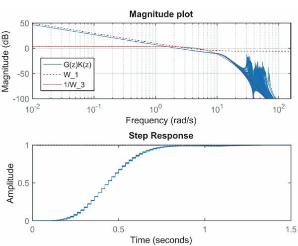
Figure 7 Magnitude plots and step responses for 100 random parameter sets.

Table 3 Controller parameters

Sampling period TS	20 ms
Faster sampling period used in the force filtering	2 ms
Time constants of the low-pass filters	50 ms
Feedforward gain KFF	0.8
Torque threshold τ tol	1 Nm
Wp	2×10–15 Nm Pa–3s m–3
Minimum pressure for accumulator 2	6 MPa
Target pressure for accumulator 2	7 MPa
Minimum pressure for accumulator 3	12 MPa
Target pressure for accumulator 3	13 MPa

The other controller parameters are given in Table 3. The sampling period is selected according to the response time of the logic valves. Because the inverter delay is 30 ms, the total delay of the controller (k in Equation 23) is two sampling periods. The time constants of the low-pass filters are tuned such that repetitive mode switching and bilge pump starts are avoided. The feedforward gain is selected such that the nominal response has no over-or undershoot. The torque threshold is selected to be as small as possible but such that repetitive mode switching is avoided. Parameter W_p of the cost function is tuned such that the accumulator pressures remain near target values. The target pressure for accumulator 3 is selected such that responses with high load forces are possible. The target pressure for accumulator 2 is selected rather arbitrarily; the selection may have an effect on performance and losses.

Simulated Results

Nominal Responses

The nominal system has three accumulators, 49000 kg load mass and 1100 MPa bulk modulus. The load force is either 9 kN, –18 kN or 36 kN. The fifth-order polynomial is used as the position reference. Figure 8 presents the simulated response with 9 kN load force. The left column shows the simulated and target piston positions, the simulated and target rotational speeds, pressures at the accumulators, the torque of the electric motor and the control signal of the bilge pump. Value one means that the bilge pump is stopped, value two that it is pumping into accumulator 2 and value three that it is pumping into accumulator 3. The right column presents the simulated and target piston velocities, chamber pressures, pressures at volumes C and D, the output power of the electric motor and cylinder actuator and the control signals of the logic valves. When compared to the previous studies with the same loading system and reference, the tracking performance is excellent. The peak torque of the system remains below 10.4 Nm, and the peak power of the electric motor is 2.2 kW. The mechanical output power is relatively small, because of the small load force. Figure 9 shows the simulated response with –18 kN load force. The performance is quite similar. The peak power of the electric motor is 1.9 kW, while the peak power of the actuator is 3.3 kW. Figure 10 presents the simulated response with 36 kN force. The peak power of the electric motor increases to 2.9 kW, while the peak power of the actuator is 4.5 kW.

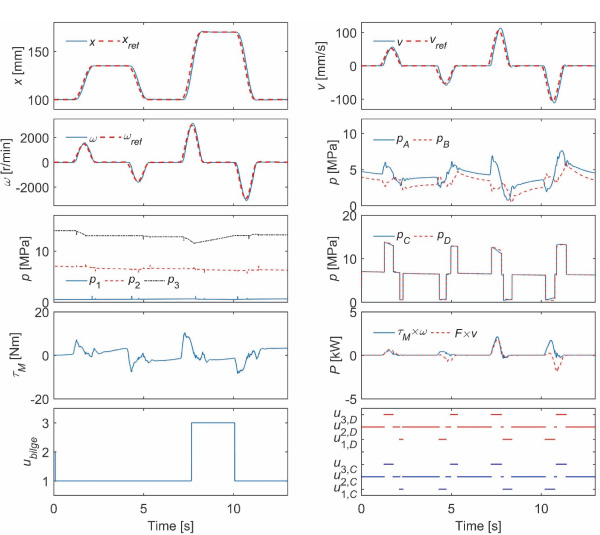
Figure 8 Nominal response with 9 kN load force.

Results with Different Numbers of Accumulators

Figure 11 shows the simulated responses for 36 kN load force when only the low-pressure accumulator is used (N = 1), when the low-pressure and high-pressure accumulators are used (N = 2), and when three accumulators are used (N =3). It is seen that the response with one accumulator is smooth, but the peak torque is 22.5 Nm. The response with two accumulators has strong transients, and the peak torque is 22.1 Nm. The switching between low and high pressure causes big torque disturbances on the electric servomotor, which results in large velocity transients. Three accumulators again produce a smooth response, and the peak torque is only 10.6 Nm. It can be concluded that at least two additional pressure sources are recommended and that the peak torque is reduced by 52 per cent in this case.

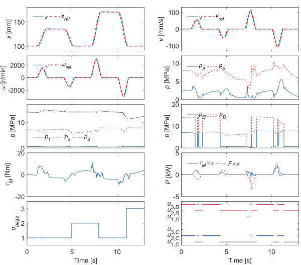
Figure 9 Nominal response with –18 kN load force.

Robustness

The robustness is studied by simulated step responses. The load force is 9 kN, and the number of accumulators is three. The following parameter sets are used:

1. m = 49000 kg, B_A =B_B = 800 MPa, x_ref = 0.17 m (minimum natural frequency)
2. m =10450 kg, B_A = B_B =1400 MPa, x_ref = 0.05 m (close to maximum natural frequency)

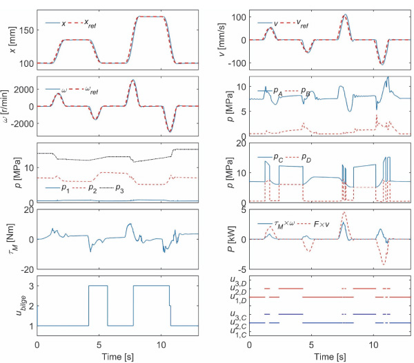
Figure 10 Nominal response with 36 kN load force.

Figure 12 presents the 20 mm step responses. Both responses are stable and close to each other. The rise time is similar, but the overshoot is slightly larger than predicted by the linearized model (Figure 7). The simulations prove that the system is robustly stable.

Energy Consumption

Table 4 summarizes the energy consumption of the system when three accumulators are used. The results are obtained by simulating ten consecutive responses similar to those in Figures 8–10. Energies are obtained from powers by integration. The output power of the electric servomotor is calculated as the product of the torque and the rotational speed; electrical losses are thus excluded. The bilge pump is assumed to be ideal, and its power is calculated as a product of flow and pressure. The mechanical output power is the product of the piston velocity and force calculated from the chamber pressures. The energy released from the accumulators is calculated by integrating the flow from the accumulator times the pressure in the accumulator. Finally, the energy loss is calculated by summing energies supplied by electric servo motor, bilge pump and accumulator, and subtracting the mechanical output energy from this value. A significant amount of input energy is inserted into the system via the bilge pump. Its role is to charge the accumulators, and the power is a maximum 500 W. The electric servomotor performs the motion control and has peak power up to 2.9 kW. The characteristic energy consumption is 15.6–16.0 J mm^–1, good values for this system. Characteristic power consumption with the same system has been measured at 45 J mm^–1 with electric load sensing and a mobile proportional valve (Linjama et al., 2007), at 29 J mm^–1 with electric load sensing and distributed digital hydraulic valves (Linjama et al., 2007), at 19 J mm^–1 with a secondary controlled multi-chamber cylinder (Linjama et al., 2009) and at 11.9 J mm^–1 with a multi-pressure hybrid actuator (Huova et al., 2017). It is important to note that pump losses are ignored in the abovementioned research, while realistic loss models are used in this paper for the pump motors.

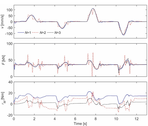
Figure 11 Simulated responses when the number of supply pressure is varied. Load force is 36 kN.

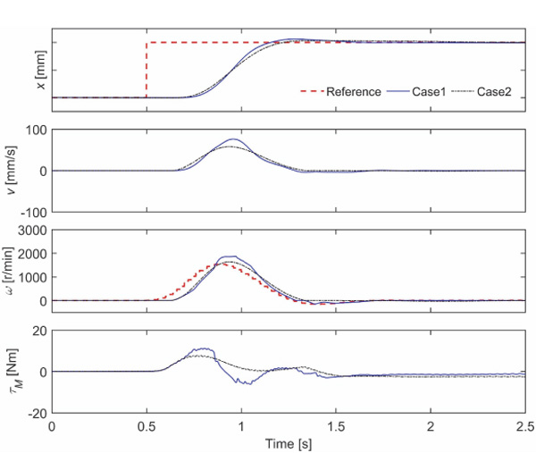
Figure 12 Simulated 20 mm step responses with two different parameter sets.

Table 4 Simulated energies for ten consecutive responses

	9kN	–18 kN	36 kN
Electric servo motor	17.1 kJ	18.8 kJ	23.0 kJ
Bilge pump	16.1 kJ	15.2 kJ	12.4 kJ
Mechanical output energy	1.2 kJ	1.2 kJ	1.1 kJ
Energy from accumulators	0.8 kJ	0.5 kJ	–0.6 kJ
Energy loss	32.8 kJ	33.3 kJ	33.6 kJ
Energy loss per stroke mm	15.6 J mm–1	15.9 J mm–1	16.0 J mm–1

Conclusions

The simulation results of this paper show that it is possible to implement a variable speed drive with small input power and large output power by using hydraulic accumulators to generate balancing torque. When three 1 l accumulators are used (one of them being a pressurized tank), the torque required from the electric servomotor is reduced by 52 per cent. The control performance is excellent with the proposed robust controller. The controller is also robust against large variations in the load mass, bulk modulus and friction. The hydraulics of the solution is somewhat complex, because a small bilge pump, two pump motors and three accumulators are needed. The geometric displacements of the pump motors must also closely match with the cylinder areas. In this case, a sufficient match was achieved with existing components, but in general, a cylinder with a non-standard piston rod diameter may be needed. These challenges must be weighed against the reduced size and price of the electric servomotor as well as good energy efficiency and excellent controllability.

Acknowledgement

The research was supported by the Academy of Finland under Grant number 278464.

References

Anon. 2017. GVM Global Vehicle Motor – Permanent Magnet (PMAC) Motors and Generators for Traction, Electro-Hydraulic Pump (EHP) and Auxiliary Systems, Brochure 192-300108N6, Parker Hannifin Corporation, October 2017.

Belda, K. 2013. Mathematical Modelling and Predictive Control of Permanent Magnet Synchronous Motor Drives. Transactions on Electrical Engineering, 2, 114–120.

Boes, C. and Helbig, A., 2014. Electro Hydrostatic Actuators for Industrial Applications. In: H. Murrenhoff, ed. 9th International Fluid Power Conference, 24–26 March 2014 Aachen. Aachen: Fördervereinigung Fluidtechnik e.V., 134–142 (Vol. 2).

Canudas de Wit, C., et al., 1995. A New Model for Control of Systems with Friction. IEEE Transactions on Automatic Control, 40, 419–425.

Filatov, D., Minav, T. and Heikkinen, J. 2018. Adaptive Control for Direct-Driven Hydraulic Drive. 11th International Fluid Power Conference, 19–21 March 2018 Aachen. Aachen: RWTH Aachen University, 110–118 (Vol. 1).

Huova, M., et al., 2017. Digital Hydraulic Multi-Pressure Actuator – The Concept, Simulation Study and First Experimental Results. International Journal of Fluid Power, 18, 141–152.

Huova, M., et al., 2018. Fuel Efficiency Analysis of Selected Hydraulic Hybrids in a Wheel Loader Application. Bath/ASME Symposium on Fluid Power and Motion Control, 12–14 September 2018 Bath. The American Society of Mechanical Engineers, 10 p.

Ketonen, M. and Linjama, M. 2017. High Flowrate Digital Hydraulic Valve System. The Ninth Workshop on Digital Fluid Power, 7–8 September 2017 Aalborg. Aalborg University, 13 p.

Koitto, T., et al., 2018. Experimental Investigation of a Directly Driven Hydraulic Unit in an Industrial Application. 11th International Fluid Power Conference, 19–21 March 2018 Aachen. Aachen: RWTH Aachen University, 348–361 (Vol. 2).

Leinamo E. 2018. Hydraulisen Testijärjestelmän Toteutus Kestomagneettimoottorin Kuormitushäiriöiden Tutkimiseksi. MSc thesis, Tampere University of Technology, Finland, 2018. http://URN.fi/URN:NBN:fi:tty-201802231312 (in Finnish).

Linjama, M., et al., 2007. Design and Implementation of Energy Saving Digital Hydraulic Control System. In: J. Vilenius, K.T. Koskinen and J. Uusi-Heikkilä, ed. Proceedings of the Tenth Scandinavian International Conference on Fluid Power, 21–23 May 2007 Tampere. Tampere: Tampere University of Technology, 341–359 (Vol. 2).

Linjama, M., et al., 2009. Secondary Controlled Multi-Chamber Hydraulic Cylinder. 11th Scandinavian International Conference on Fluid Power, 2–4 June 2009 Linköping. Linköping: Linköping University, 15 p.

Linjama, M., et al., 2015. Hydraulic Hybrid Actuator: Theoretical Aspects and Solution Alternatives. 14th Scandinavian International Conference on Fluid Power, 20–22 May 2015 Tampere. Tampere: Tampere University of Technology, 11 p.

Mare, J.-C., 2010. Towards More Electric Drives for Embedded Applications: (Re)discovering theAdvantages of Hydraulics. In: H. Murrenhoff, ed. 7th International Fluid Power Conference, 22–24 March 2010 Aachen. Aachen: Apprimus Verlag, 75–86 (Vol. 4).

Minav, T., et al., 2014. Direct Driven Hydraulic Drive. In: H. Murrenhoff, ed. 9th International Fluid Power Conference, 24–26 March 2014 Aachen. Aachen: Fördervereinigung Fluidtechnik e.V., 520–529 (Vol. 2)

Müller, K. and Dorn, U., 2010. Variable Speed Drives – Customer Benefits in Injection Molding Machines and Presses. In: H. Murrenhoff, ed. 7th International Fluid Power Conference, 22–24 March 2010 Aachen. Aachen: Apprimus Verlag, 165–176 (Vol. 4).

Paloniitty, M., Linjama. M. and Huova. M. 2018. Compact and Efficient Implementation of a Pressurized Tank Line. White paper, http://urn.fi/URN:NBN:fi:tty-201811262768.

Tikkanen, S. and Tommila, H. 2015. Hybrid Pump Drive. 14th Scandinavian International Conference on Fluid Power, 20–22 May 2015 Tampere. Tampere: Tampere University of Technology, 11 p.

Zhang, S., Minav, T. and Pietola, M., 2017. Improving Efficiency of Micro Excavator with Decentralized Hydraulics. In: ASME/BATH 2017 Symposium on Fluid Power and Motion Control, 16–19 October 2017 Sarasota. The American Society of Mechanical Engineers, 8 p.

Biography

Matti Linjama obtained a D Tech degree at Tampere University of Technology, Finland in 1998. Currently, he is an adjunct professor at the Automation Technology and Mechanical Engineering Unit, Tampere University. He started the study of digital hydraulics in 2000 and has focused on the topic since then. Currently, he is leader of the digital hydraulics research group and his professional interests include the study of hydraulic systems with high performance and energy efficiency.

International Journal of Fluid Power, Vol. 20 1, 125–150.
doi: 10.13052/ijfp1439-9776.2015
© 2019 River Publishers

Abstract

Introduction

System Model

Electric Servomotor and Inverter

Pump Motors

Accumulators, on/off Valves and Bilge Pump

Volumes between Valves and Pump Motors

Cylinder Actuator and Check Valves

Controller Design

Linearized Model of the System

Robust Controller Design

Control of Balancing Torque

Closed-loop Position Control

Control of Bilge Pump

Simulated System

Controller Tuning

Simulated Results

Nominal Responses

Results with Different Numbers of Accumulators

Robustness

Energy Consumption

Conclusions

Acknowledgement

References

Biography