Computational Valve Plate Design in Axial Piston Pumps/Motors
Paul Kalbfleisch* and Monika Ivantysynova
Purdue University, School of Mechanical Engineering, 585 Purdue Mall,
West Lafayette, Indiana 47907-2088, USA
E-mail: pkalbfle@gmail.com
* Corresponding Author
Received 04 February 2019; Accepted 28 August 2019; Publication 19 September 2019
Abstract
Many industries utilize axial piston machines for the compact design, high operating pressures, variable displacements, and high efficiencies that far outweigh the machines’ manufacturing costs. For all axial piston machines, the valve plate functions as an essential determinant of performance. The aim of this research is to develop a design methodology generalizable to all types of valve plates while remaining accessible to users without advanced technical knowledge. The proposed design methodology is organized to fit the form of the standardized optimization problem statement. This organization enables the use of any modern optimization algorithm. Specifically, the design methodology utilizes a previously developed computer model, which is based on the main physical phenomena influencing the design of flow passages from the pump port to the displacement chambers and vice versa. The chosen design methodology allows the precise optimization of the valve plate design by simulations rather than expensive trial and error processes. A recent case study demonstrated the strong positive correlation between application of the methodology and improved performance of the valve plate design.
Keywords: Valve plate, optimization, positive displacement, axial piston machine, relief grooves, noise, vibration.
1 Introduction
In swashplate-type axial piston machines, the pistons are supported on the swash plate, and the cylinder block usually rotates while the swash plate is stationary (Figure 1). The valve plate connects the individual displacement chamber with the high-pressure and low-pressure port.
As each displacement chamber rotates around the shaft, the valve plate connects the displacement chamber to the suction port or to the discharge port, or to both. Consequently, the valve plate design defines the time of connection between each displacement chamber to the pump/motor high-pressure and low-pressure port. In order to achieve a desired pressure gradient of rising the pressure from low to high pressure or visa versa relief grooves are often introduced.
The relief grooves, as shown in Figure 2, help control the flow entering from the suction or discharge port to the displacement chamber with respect to its piston position. By changing the position and size of the relief grooves the opening/closing time, the amount of flow can be influenced. This will influence the pressure rise/fall in each displacement chamber, which in turn impacts the pump/motor operation. This paper proposes a computationally based design methodology to optimize the valve plate design with respect to the pump/motor performance and noise emissions.

Figure 1 Axial piston swash plate pump.
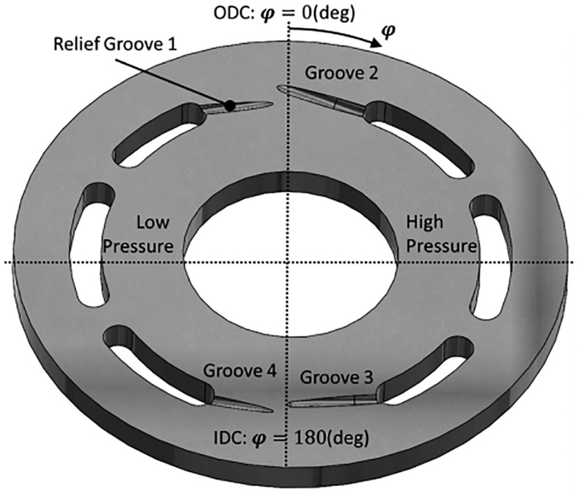
Figure 2 Valve plate with groove numbering.
2 State of the Art
The motivation for valve plate design optimization has been predominantly pushed by increasing requirements to reduce noise emissions of the machines. This valve plate optimization can be used to reduce both structure-borne noise sources (SBNS) and fluid-borne noise sources (FBNS). Many researchers have investigated fluid borne noise and structure borne noise generated in positive displacement machines. A comprehensive review about past researcher can be found in Edge (1999) and Seeniraj (2009).
Valve plate design was first considered for the reduction of fluid-borne noise sources in the summaries of reduction techniques and their limitations completed by Harrison (1997) and Johansson (2005). The simplest reduction technique is ideal timing. Ideal timing indicates the intentional delay of the opening between the displacement chamber and each of the ports. However, using ideal timing to achieve compression is effective only for a particular pressure level and for a specific displacement (Helgestad, 1974; Pettersson, 1991; Yamauchi, 1976; Pettersson, 1995; M.E. Pettersson, 1995; Zhang et al., 2009; Schleihs et al., 2014; Frosina et al., 2018; Ye, Zhang and Xu, 2018). Alternatively, relief grooves were found to be less sensitive to pressure levels and speeds than ideal timing. Relief grooves spread out the compressibility effect throughout multiple operating conditions (Harrison, 1997; Pettersson, 1991). Relief grooves achieve compression using high-pressure fluid from a discharge port. Rate of compression is controlled by geometry of relief grooves, limiting back flow from discharge port into displacement chamber (Palmberg, 1989). Achieving compression with fluid from a discharge port creates a strong positive correlation between groove geometry and flow ripple. Further, relief grooves influence volumetric efficiency if there is cross porting between discharge and suction ports (Pettersson, 1991).
Seeniraj (2009) developed a design methodology for valve plates in swash plate-type axial piston machines at the Maha Fluid Research Center. Convinced by Edge’s summary of fluid power noise research (1999), Seeniraj developed a design methodology to reduce both structure-borne noise sources and fluid-borne noise sources. This led Seeniraj to the field of multiobjective optimization. Multiobjective optimization attempts to minimize multiple objective functions (performance parameters) simultaneously. There will be, at some point, a subjective decision made, in order to choose the priority of the various objective functions.
Seeniraj (2009) sampled the operating conditions (Opcons) in order to estimate the entire operating condition range with only a few simulated conditions. He conservatively chose the eight extreme corner operating conditions of a pump.
Seeniraj’s design of experiments would be classified as a combination of a full factorial search and grid search. A true full factorial design of experiments does not require changing of the “parameter intervals.” Seeniraj’s methodology requires a human in the loop every few hours. This requires the user of the algorithm to be present at the computer/work in order for the algorithm to continue. In computer science, this process is known as a barrier and requires the entire algorithm to pause while waiting for the input of the user. In this paper, a methodology is proposed that removes the barrier.
Previous research conducted in the field of optimization presents an enormous amount of literature for scholastic consideration.
Blum and Roli (2003) provide a detailed overview and comparison of the many different metaheuristic methods involved in combinatorial optimization. Blum and Roli (2003) list a few famous metaheuristic algorithms, including (but not limited to)Ant Colony Optimization (ACO); Evolutionary algorithms (EA), including Genetic Algorithms (GA); Iterated Local Search (ILS); Simulated Annealing (SA); and Tabu Search (TS).
Two concepts in particular lend themselves directly to the development of the methodology presented in this paper: non-domination sorting (rank) and the crowding distance metrics (Deb, 2002).
3 Simulation Model
The simulation model is based on the utilization of a control volume approach. Figure 3 shows the control volume considered for the displacement chamber. The control volume is used to calculate the instantaneous pressure in the displacement chamber.
| (1) |
A lump parameter pump model calculates the individual flow of all the displacement chambers to and from both the HP port and LP port. QSKi represents the leakage flow rate between each piston and cylinder. QSBi represents the leakage flow rate between the cylinder block and valve plate. QSGi represents the leakage flow rate through the piston bore to the slipper. QSKi, QSBi, and QSGi can be set to zero when neglecting the effect of external leakages.
| (2) |
Qri represents the volumetric flow into a single displacement chamber and is calculated by summing the fluid flow between the displacement chamber and each port (HP port and LP port) (Equation 1).
QrHPi represents the volumetric flow from a single displacement chamber to the HP port. QrLPi represents the flow to a single displacement chamber from the LP port as described in Figure 3. Both flows are assumed to have high Reynolds numbers and are modeled using the orifice equation. A positive flow represents fluid flowing into the displacement chamber, and a negative flow represents fluid flowing out of the displacement chamber.
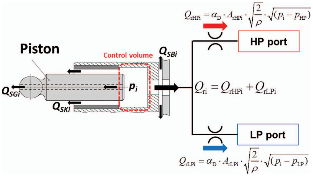
Figure 3 Control volume of displacement chamber (Kim, 2014).
The valve plate area openings at a given rotating angle of the shaft (ArLPi and ArHPi) are incorporated into the model through the use of a predefined lookup table. This lookup table includes both an ArLPi and ArHPi for a set number of discrete angular positions of the cylinder block, i.e. time steps. ArLPi and ArHPi are defined as the minimum cross-sectional area perpendicular to a streamline of the flow at each angular position from the port through the valve plate opening to the displacement chamber. The areas in between the table values are created by linear interpolating within the table. This table is external to the model, and is referred to as an Area file.
For an existing design, the area file is measured from the geometry of the pump. An additional software AVAS (Ivantysynova, 2004) was developed using a given CAD geometry and computational fluid dynamics (CFD) to automatically calculate these areas. AVAS calculates a single streamline using CFD and takes consecutive cross-sectional areas of the fluid volumes in order to find the smallest cross-sectional area.
A magnified image of the areas around Outer Dead Center (ODC) and Inner Dead Center (IDC) is emphasized in Figure 4 due to its enormous influence on the operation of the pump. It is only during expansion and compression of the fluid around ODC and IDC that the orifice flows, formed by restricted relief grooves areas, play a role in determining the pressure of the displacement chamber. The Area file will become the most crucial input to the pressure module, as the design of a particular valve plate can be completely characterized by a given Area file (assuming no change in the cylinder block). Therefore, the rest of this paper will be centered on the design of the Area file.
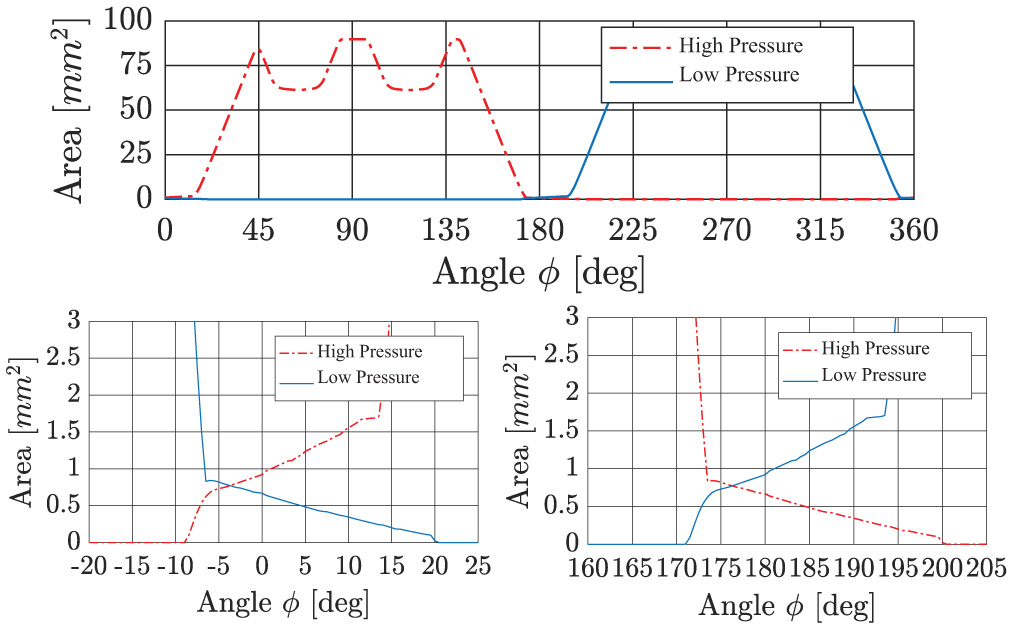
Figure 4 Example area file.
The total fluid model used in order to calculate displacement chamber pressure is shown in Figure 5. Notice that each box is a single fluid control volume, and all the fluid within each control volume is assumed to be at the same pressure, as this model is a lumped parameter model. This model is, therefore, a system of ordinary differential equations. Each fluid volume’s pressure is described using a single differential equation in all the fluid volumes being coupled by the connective orifice flows. The entire system is referred to as the pressure module. The essential outputs of the pressure module are the resulting instantaneous inlet and discharge flows and port pressures for an entire shaft revolution.
This system of ordinary differential equations is then solved using open-source numerical solvers. An example of a general explicit method is shown in Equation 3.
| (3) |
This particular system of ordinary differential equations dramatically varies its stiffness. An ordinary differential equation problem is stiff if the solution being sought is varying slowly, but there are nearby solutions that vary rapidly. As a result, the numerical method must take small steps to obtain satisfactory results. The current publicly available solver used here is the LSODA solver. LSODA is the acronym for Livermore Solver for Ordinary Differential Equations:Automatic method selection. It is a variant of the solver LSODE (Livermore Solver for Ordinary Differential Equations) developed by Linda R. Petzold (1983).
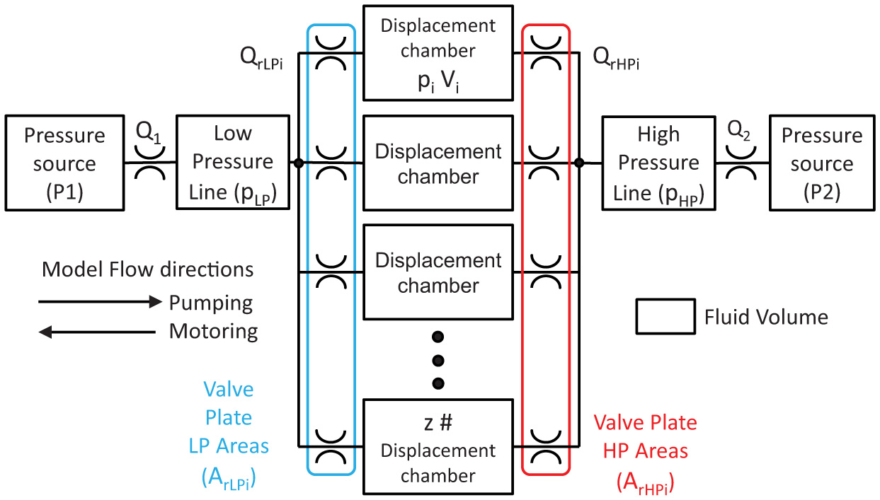
Figure 5 Simulation set-up for modeling of the displacement chamber pressure.
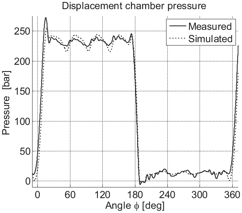
Figure 6 Example displacement chamber pressure.
Figure 6 shows an example for the calculated displacement chamber pressure as a function of the rotation angle phi. Measurements using a piezo electric pressure sensor mounted directly in the displacement chamber and a telemetry unit to transfer the signal from the rotating cylinder block was made in order to compare the simulation results and to verify the correctness of the pressure module. Figure 6 shows the comparison of the measurement and simulation displacement chamber pressure (Wieczorek, 2000). This will be used to calculate most of the performance parameters of the given valve plate design.
The effective discharge flow rate (Qe) (Figure 7), includes the kinematic flow ripple, compression of the fluid, external leakages, and the effect due to cross porting of the valve plate. The combination of cross porting and fluid compressibility greatly increases the peak to peak (maximum - minimum) amplitude of the discharge flow. This amplitude (ΔQhp) is referred to in the literature as the fluid-borne noise source (FBNS). The flow ripple generated by the pump transmits throughout the entire hydraulic system, inducing vibrations through other components and potentially causing airborne noise (ABN) detectable by human ears. The flow ripple generates pressure ripples in the hydraulic lines. These pressure ripples create proportional force ripples, which can cause violent oscillations in the physical structure of the machine.
To distinguish from the true volumetric losses (Qs), leakage* is introduced to refer only to the internal leakages (due to cross porting and compression losses).
| (4) |

Figure 7 Example discharge flow ripple.
Similarly, to distinguish from true volumetric efficiency, a term is defined as volumetric efficiency* .
| (5) |
Where, the geometric flow (Qgeo) is determined by summing all piston’s geometric displaced volume. These are calculated by the product of each piston’s area and its piston stroke. The effective discharge flow only includes internal leakages and excludes external leakages such as gap flows (QSKi, QSBi, and QSGi).
| (6) |
Figure 8 shows the instantaneous volumetric efficiency* for one revolution of a 44cc pump (example valve plate).
The resulting pressure force of all pistons and its point of application is known and allows the calculation (see Ivantysn and Invantysynova, 2004) of the swash plate moments MX, MY and MZ exemplified in Figure 9. The oscillating force and moments create vibrations of the solid parts of an axial piston machine and are a major source of what is referred to in the literature as structure-borne noise sources (SBNS).
| (7) |

Figure 8 Example volumetric efficiency*.
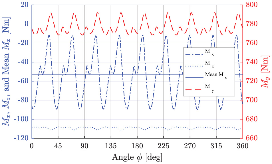
Figure 9 Example swash plate moments.
| (8) |
| (9) |
The force (Fpi) in Equations 7–9 is composed of the pressure and inertial forces, applied by each piston to the swash plate. The friction force is small compared to the pressure force and the inertia force (Lasaar and Invantysynova, 2004) and can therefore be neglected while studying the structure-borne noise sources.
The combination of the Fpi creates oscillations and unwanted periodic vibrations of the swash plate, which get transferred to the exterior case in the surrounding structures. The specific structure response and acoustic radiation will additionally attenuate far-field sound pressure. The peak-to-peak amplitude of each oscillating moment precisely quantifies the structure-borne noise source (ΔMx and ΔMy).
The optimization algorithm can also be used to optimize a design with respect to the mean of the moment Mx. The moment Mx forms an important design parameter for the pump control system: The pump control system has to be designed to overcome the mean value of Mx. An increased mean Mx is seen as a disadvantage, because it causes an increase of the required pump control system power. In case of a manually operated pumps large mean value will lead to fatigue of the human operator.
4 Valve Plate Design Space
As previously explained, the geometry of the valve plate openings is described in the area file. The most important sections of the valve plate’s area file are at the port boundaries. The two port boundaries are labeled ODC and IDC. Each boundary has decreasing opening areas to one port, while simultaneously increasing the opening areas to the other port. The relief grooves design was introduced in order to control these boundaries with greater fidelity. It is therefore sufficient to characterize the entire valve plate geometry (area file) with the description of these important areas of flow restriction located in the regions close to ODC and IDC.
To organize the multiple relief grooves, a convention was set in order to precisely map the modeled area files to real valve plate geometries. Figure 2 shows the groove numberings relative to the conventional coordinate system defined at the Maha Fluid Power Research Center when the displacement unit is operating in pumping mode.
A new category of nonlinear area file shapes is introduced in this paper. The improvement from traditional linear to nonlinear grooves came about for three reasons. First, some valve plates cannot physically be manufactured with linear grooves. Second, previous research with linear grooves demonstrated that grooves with an “offset” have better ΔMx performance (Seeniraj, 2009). Last, the circular nature of the nonlinear groove derives from the common practice of manufacturing valve plates by cutting the surface of the plates using ball end mills. The manufacturing of a nonlinear groove does not require the changing on the manufacturing process of linear grooves. The nonlinear start translates into drilling slightly deeper at the beginning of the grooves.
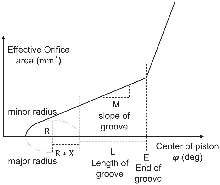
Figure 10 Nonlinear groove shape (area file).
The specific set of variables that parameterize the nonlinear groove shape were chosen for three main reasons. First, these specific variables provide essential aid to the optimization algorithm in making correlations between inputs and outputs. Second, variable orthogonality, or variable independence, played a major role in variable selection. Third, the current set of parameterization variables allows the designer to easily limit the possible designs to older reduction techniques, such as ideal timing and linear relief grooves (Figures A1 and A2).
Historically, it was common to assume certain symmetry of the valve plate (grooves) in order to simplify the design process. Experience from previous design studies revealed a compromise that could not be avoided using the traditional symmetric groove constraint. The constraint of symmetric grooves required a choice between pressure peaks at ODC or IDC. This was the motivation to decouple the ODC and IDC grooves, thus creating asymmetric grooves. Asymmetric grooves simply describe a set of four grooves wherein each has been designed independently.
5 Optimization Problem Statement
The design of a valve plate can be a subjective task. First, the precise problem to be solved must be clearly defined. In general, a mathematical optimization problem consists of minimizing an objective function, f, which is a function of a set of design variables, .
Each groove is defined by five variables. Therefore, every design using asymmetric nonlinear grooves has 20 design variables for the valve plate and an additional eight for the filter volumes. The input vector is 28 variables long.
| (10) |
The design of a valve plate is one example of the class of optimization problems known as Multiobjective Optimization. Multiobjective optimization is the field of minimizing multiple objective functions simultaneously. The objective functions are based on the previously discussed performance parameters. The performance parameters have been defined in such a way as to facilitate efficient translation into objective functions. Currently, there are five performance parameters used for objective functions. All five of these performance parameters are defined such that minimizing these functions increases the performance of the pump.
Minimize: For All Operating Conditions
| (11) |
| (12) |
| (13) |
| (14) |
| (15) |
It is extremely important to understand that the full optimization problem statement includes minimizing for all operating conditions. This is a theoretical problem statement; in reality, the operating conditions must be sampled in order to approximate the entire space.
Within a multi-objective problem, design A can only be certainly better then design B if all of design A’s objective function values are smaller than all of design B’s objective function values. This is defined as A dominates B. The set of all designs that are not strictly dominated by any other design are termed non-dominated designs. Non-dominated designs are also referred to as Pareto optimal. The set of all Pareto optimal designs form the Pareto front.
An example Pareto front from a well-known multi-objective optimization problem, ZDT1 (Zitzler et al., 2000), is shown in Figure 11.
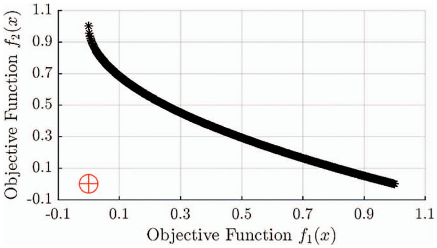
Figure 11 ZDT1 Pareto front.
An important term to define is the utopian point. The utopian point (Figure 11, red dot) is not a real design, but is the perfect solution to the multi-objective problem. The creation of the utopian point involves taking the smallest value from every objective function independently along the Pareto front and creating a single utopian point. The utopian point functions as a useful benchmark for determining the ideal manifestation of each objective function.
Most real-world applications require additional constraints to be placed upon the design variables. These constraint functions are also functions of the design variables. There are five inequality constraints and one equality constraint. All the constraints are each bounded by a separate limit variable, L. These limit variables are set in the beginning and remain constant throughout the running of the optimization algorithm.
| (16) |
| (17) |
| (18) |
| (19) |
| (20) |
| (21) |
The constraints were created in order to ensure a correct convergence of the solution (g3, g4, g5, and h1) and to guide the optimization algorithm towards a feasible solution.
6 Operating Condition Sampling
This paper next addresses sampling of operating conditions in order to estimate the whole operating range for the objective functions and constraints. The amount of operating conditions yields substantial influence on the total time needed to evaluate each valve plate design. The time needed is linearly proportional to the number of operating conditions simulated.
In order to show all the operating conditions in a single figure, a new type of plot has been introduced (Figure 12). This plot is, in short, referred to as an Opcon plot. A total of 1800 operating conditions are simulated for a single design and combined into a single graph. Each Opcon plot displays a single performance parameter.
Beginning with constraints g1 and g2, both the maximum pressure and minimum pressure extrema (above/below the average port pressures) occur at the same operating condition. This operating condition is the highest speed, highest displacement angle, and lowest Δpressure.
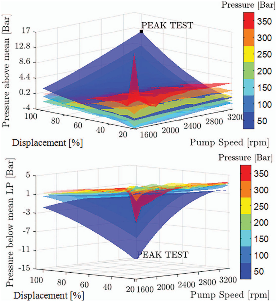
Figure 12 Opcons plot: Example “Peak Test” for maximum and minimum pressures.
As per Equation 1, the dv/dt term of the pressure buildup equation is the only term that can create pressures in the displacement chamber that are not between the port pressures. The dv/dt term increases with speed and swash plate angle. The orifice flows to/from the ports will always lead the displacement chamber pressure to a pressure equal to the corresponding port. The port orifice flows always reduce pressure peaks above/below the port pressures. The port orifice flows are based on the differential pressure (Figure 2) and are therefore minimized at the lowest high pressure. The pressure extrema will always be the worst at the peak test operating condition. The constraint for pressure extrema needs only be performed at this operating condition.
Similar to the pressure extrema, the volumetric efficiency* minimum always occurs at a consistent operating condition. This operating condition occurs at the lowest speed, lowest displacement, and highest Δpressure of interest (Figure 13). The volumetric efficiency’s* minimum always occurs at this operating condition because of cross porting (Kim, 2014).
Research completed by Klop (2010), showed that the noise generated by pump/motor is roughly proportional to the fluid power transmitted. Therefore, the first operating condition to consider is the maximum power.
A case study was performed to determine the minimal amount of simulated operating conditions in order to approximate the entire operating condition range. The study used ΔMx as the example performance parameter, because it is most influenced by the operating conditions. Minimizing the maximum power operating condition (OPCON A) had a negative effect on other operating conditions. In order to give control of this effect to the user, another operating condition must be chosen. In order to minimize the number of operating conditions simulated, the volumetric efficiency* constraint operating condition (OPCON C) was chosen because it will already be simulated. It was shown that the tested optimization algorithm could reduce the objective functions for the entire operating condition space using only two (A and C) sampled operating conditions (Figure 14).
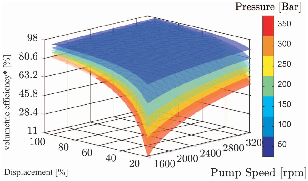
Figure 13 Opcon plot: volumetric efficiency.
It is always recommended to create the Opcon Plots in post processing to verify the success of the Opcon sampling. The current trends, using only two opcons, are dependent on the possible designs of groove geometry. More complicated groove geometries will enable the operating conditions influence on the performance parameters in a more complex way.
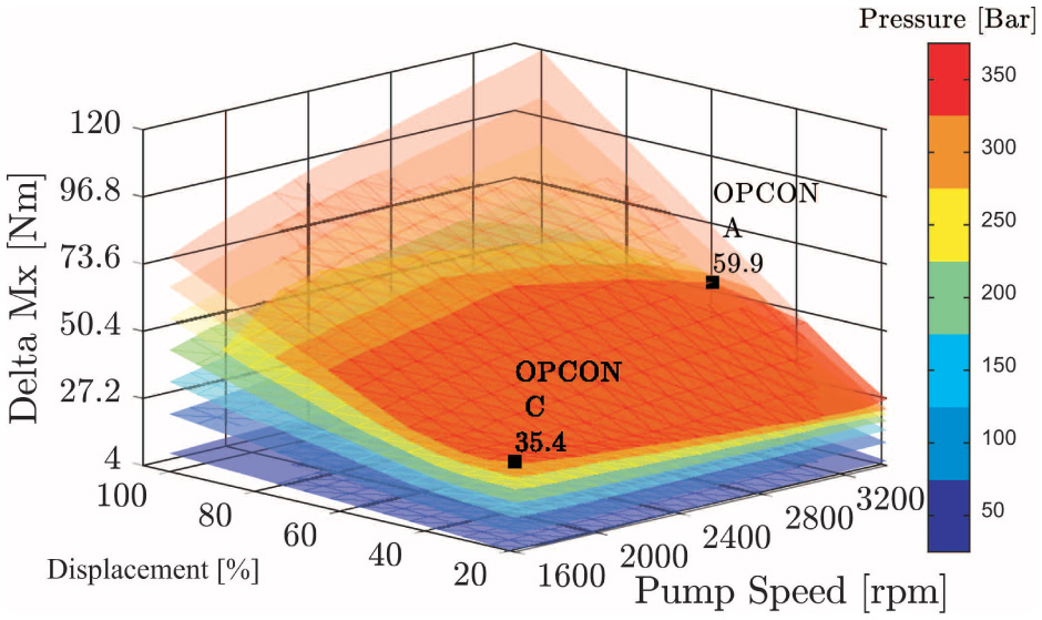
Figure 14 Opcon plot: ΔMx; 2 Opcons sampled.
Table 1 Problem statement summary
| A | B | C | |
| Leakage* [%] | |||
| ΔQhp | |||
| ΔMx | |||
| ΔMy | |||
| Max pressure | * | ||
| Min pressure | * | ||
| Leakage* | * | ||
| |HP mean – set| | * | * | * |
| |LP mean – set| | * | * | * |
| Finished Simulation | * | * | * |
To summarize the valve plate design problem statement, there are five objective functions and six constraint functions simulated at the three different operating conditions, labeled below.
A. Maximum Unit Power (Application)
B. max n, min Δp, max β
C. min n, max Δp, min β
7 Design Methodology
Non-dominated sorting genetic algorithm II (NSGA-II) is the selected optimization to solve the valve plate optimization problem (VpOptim). NSGA-II satisfies all the necessary constraints given by the valve plate design problem. The main characteristic of NSGA-II is the novel solution of combining any multi-objective optimization problem by sorting every design’s Domination Rank. A complete explanation of the algorithm is given by its creators (Deb, 2002), so it is not necessary to explain all the fine details of the algorithm. In summary, NSGA-II satisfies the following necessities: It solves multiobjective optimization problems, global optimization problems, and it can be parallelized.
Figure 15 summarizes the entire proposed design methodology, including the implementation of the selected optimization algorithm (NSGA-II).
Before starting the NSGA-II algorithm, the designer must first specify the following inputs needed for the pressure module and/or the optimization algorithm. This automated methodology has enabled fewer inputs required from the designer. Those inputs are now automatically adjusted within the algorithm. This reduces the total design time needed as each input requires additional time by the designer. The following lists of inputs are required by the pressure module and are not design variables, therefore remaining constant throughout the entire design process. Only the four bold inputs contain information not readily available to the public. However, the bold inputs can be measured if the designer has access to an existing pump. This allows vehicle manufacturers to design valve plates for their machines without requiring technical information from the supplier, such as the specification of oil bulk modulus and viscosity (function of pressure and temperature), pitch diameter cylinder block, diameter piston, piston/slipper mass, max swash plate angle, number of pistons, and displacement chamber dead volume.
Second, designers will need to choose the operating conditions specific to their applications. If a designer has no experience with which operating conditions to choose, the three operating conditions (A, B, and C) will satisfy the majority of valve plate designs. The design variable limits and constraint limits given in the following case study will provide a guideline. The design variable limits given in the case study are designed to increase the variable boundaries as far as possible. It is therefore highly recommended to use the predetermined variable limits (Tables A1 and A2).

Figure 15 Design Methodology.
Finally, the two NSGA-II variables, number of generations and population size, are often incredibly difficult to determine a priori. However, the proposed new design methodology enables the designer to change these variables at the end of the optimization algorithm without having to rerun the entire optimization. It is recommended that the number of generations be set to a high number (200 to 300) because both stop and pause buttons have been implemented allowing the designer to stop NSGA-II at any generation.
The best improvement made by the current design methodology is the ability of the optimization algorithm to completely automate the optimization once the NSGA-II has begun. In this case, the NSGA-II will run for the given set number of generations and the given population size. The simulation time for a single generation will be very consistent. The designer can therefore estimate the length of the optimization routine to complete before the next work day.
The output of the NSGA-II is the set of all Pareto optimal designs of size Npop. Therefore, a single valve plate design must be chosen by the designer from the final Pareto optimal designs. This final decision made by the designer is the most abstract decision throughout the entire design methodology. This choice will be based on the designer’s priorities of the objective functions. This can be based on the specific application, measurement results, cost analysis, client preferences, and manufacturing abilities (of the valve plates). For this reason, there is a dearth of advice regarding selection of the final valve plate design. However, a safe choice from the Pareto optimal designs would include all designs that strictly dominate the original valve plate design. This would guarantee that the chosen valve plate yields better performance parameters than the original design.
8 Case Study
The proposed new design methodology was tested using a 44 cc axial piston pump. The valve plate was designed for a specific application where noise was the highest priority among the performance parameters. The given Operating conditions were chosen based on the application.
The following constraint limits were chosen and are very conservative.
| (22) |
| (23) |
| (24) |
| (25) |
| (26) |
Equality constraint(s):
| (27) |
Table 2 Case study operating conditions
| OpCon | Speed [rpm] | Displacement [%] | High Pressure [bar] | Low Pressure [bar] |
| A | 3200 | 50 | 345 | 25 |
| B | 3400 | 100 | 50 | 25 |
| C | 1600 | 20 | 345 | 25 |
The final two inputs are required for the NSGA-II algorithm. The number of generations was set to 200. The population size (Npop) was set to 450.
The optimization algorithm utilizes parallelization over multiple computers. The total number of simultaneous simulations was 120 threads. Each valve plate took, on average, 30 seconds to complete a simulation. The total average simulation time per generation was roughly 1.9 minutes. The total simulation time was roughly 6 hours 20 minutes. The Pareto front generated by NSGA-II was sufficiently evenly distributed.
The output of the NSGA-II simulations is a set of 450 (Npop) Pareto optimal designs. It is extremely difficult to graphically depict 450 designs, each containing eight objective functions. Under a normal design process, the designer would select only one final design. For the purposes of elucidation, three designs were selected in order to highlight the design methodology. Creating a weighted average function of the eight objective functions and ranking the 450 designs based on chosen weights will help organize the final 450 Pareto designs.
The best ΔMxA was chosen to highlight the lowest possible ΔMXA at operating condition A. Similarly, the best ΔQhpA was chosen to highlight the lowest possible flow ripple at operating condition A. For both of these valve plate designs, a huge compromise must be made in order to drastically decrease a single objective function. Several of the other objective functions (ΔQhpA) are worse than the original design for the ΔQhpA valve plate design. This highlights the multi-objective nature of valve plate design in the consequences of neglecting some of the performance parameters. The fourth and most important Pareto optimal design chosen would be a balanced selection of all the objective functions. The comparison of the original and balanced designs area files is shown in Figure 17.
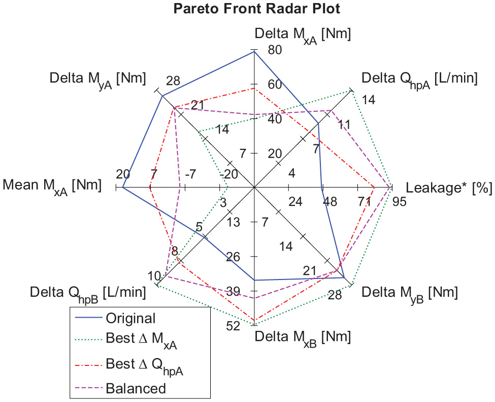
Figure 16 8 objective functions radar plot.
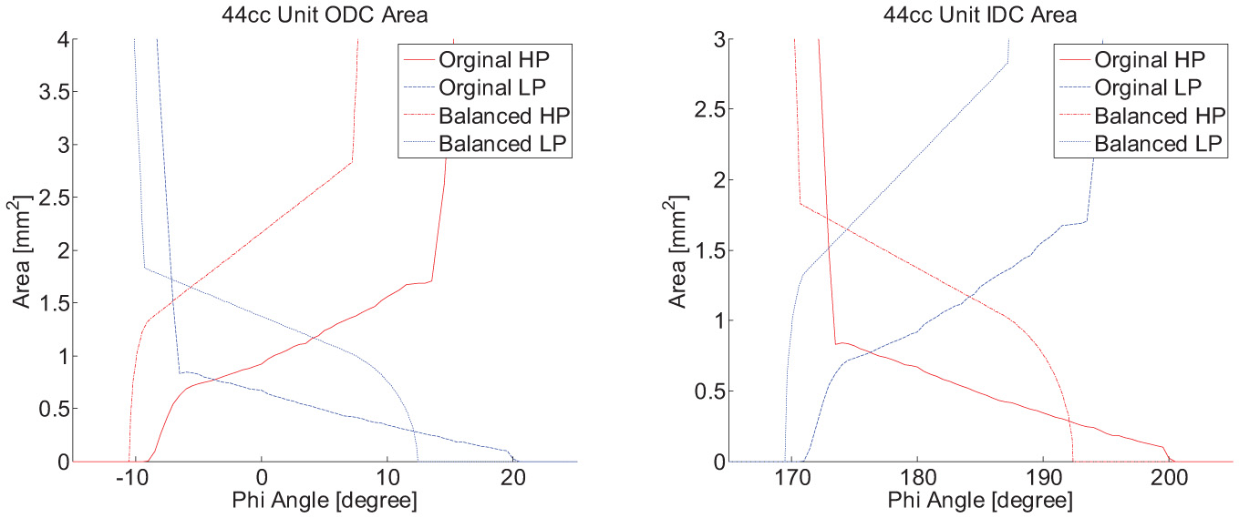
Figure 17 Balanced Vs. original area file.
The success of these results is best understood in context with the previous design methodologies. Seeniraj (2009) reached a reduced of the ΔMx by roughly 10 percent. The current reduction of 47 percent represents a more significant reduction.
This case study demonstrates the proposed design methodology’s ability to efficiently optimize multiple performance parameters, nearing the limitations of the physics modelled. The design methodology effectively populated the entire eighth dimension Pareto front, allowing the designer to simply choose the preferred priorities of performance parameters.
9 Application Specific Optimization
The proposed design methodology is an extremely fast design process as compared to the state-of-the-art in valve plate design. This design methodology enables a designer to have a large amount of control over the preferred objective functions. Moreover, the high level of control and speed enables a designer to quickly design, for the same pump, different valve plates depending on the application. The same displacement unit could be optimized for multiple machines, each requiring a different priority of the performance parameters. For example, the same pump could be installed in:
- A car where noise is very important (specifically structure-borne noise sources) and the control moment is important. The operating condition varies considerably.
- A manufacturing facility, where the fluid-borne noise sources are more important. The operating condition remains fairly constant.
- A construction vehicle, where the control moment is very important and needs to be negative (tending towards minimal displacement).
Application-specific valve plate design enables the pump manufacturer or applications engineer to customize the same pump for a wider range of applications.
To customize the vale plate design for various applications, the designer only needs to consider two components of the design methodology. The sampling of the operating conditions for each specific application; this allows the designer to narrow the optimization, considering only the usable operating range of that application (machine). As previously explained (Figure 14), minimizing a single operating condition will yield negative consequences for other operating conditions. Therefore, when minimizing multiple operating conditions, a compromise must be made. Decreasing the operating conditions base to be more specific to the application decreases the amount of compromise needed. A smaller range of operating conditions allows the designer to improve performance parameters to greater effect.
The second component of the design methodology that changes with different applications is a selection of the specific Pareto optimal design within the Pareto front. Different applications, as previously discussed, require different sets of priorities on the performance parameters.
10 Summary/Conclusions
This paper summarizes research targeted to a proposed design methodology for improving the performance of valve plates across various industries and applications. The computational model used was previously developed and verified as an accurate predictor of the valve plate’s performance. A new differential equations solver was implemented and demonstrated an increased simulation speed by 100 times, without sacrificing accuracy.
The design methodology was developed for designers that did not possess intricate knowledge of the relationship between a valve plate’s design and pump performance. The use of an optimization algorithm allows a nontechnical user to optimize a valve plate without the years of experience previously required.
The present research took further pains to ensure that the pressure module simulations in the optimization algorithm were robust to handle the vast majority of the possible errors that could occur numerically in the models.
The improvements to speed consist of a 100-times speed up from the LSODA differential equations solver, a 140 times speed up from the paral-lelization, and a subtle 8/3 speed up by reducing the number of operating conditions needed to estimate the entire operating condition space. This yields a combined speed up in simulation time of roughly 37,000 times. The parallelization architecture allows the speed up to increase linearly with the amount of computers available. Utilizing more computers would enable even greater amounts of speed improvements.
The improvements to speed and to the optimization algorithm in reducing the amount of function evaluations needed have allowed greater complexity of designs. The complexity of the valve plate designs has been increased from six design variables for the grooves to 20 design variables. This increase in complexity allows the optimization algorithm the freedom to find significantly better designs than previously allowed.
The present research highlights the performance of the design methodology. The case study involved an existing stock axial piston pump optimized for the application of a real working machine. The design methodology not only optimizes the valve plate for a specific component (displacement unit), but also takes into account the specific application (vehicle). The case study shows the success of the design methodology in substantially improving the performance parameters of a valve plate design.
Nomenclature
| ABN | Airborne noise | |
| AVAS | Automated Valve plate Area Search | |
| CFD | Computational fluid dynamics | |
| CW | Clock wise | |
| DC | Displacement Chamber | |
| FBNS | Fluid Borne Noise Source | |
| HP | high pressure | |
| IDC | Inner dead center | |
| LP | Low pressure | |
| LSODA | Livermore Solver of Differential Equations Automatic | |
| ODC | Outer dead center | |
| OPCON | Operating condition | |
| SBNS | Structure Borne Noise Source | |
| Vol Eff* | Volumetric efficiency (without external leakages) | |
| VP | Valve plate | |
| VpOptim | Valve plate optimization | |
| A | Area | [m2] |
| ArHP | Valve plate area open to discharge port | [m2] |
| ArLP | Valve plate area open to suction port | [m2] |
| Fp | Piston Pressure Force | [N] |
| I | Axial index | [-] |
| K | Fluid Bulk modulus | [Pa] |
| Mx | Swash plate moment about X axis | [Nm] |
| My | Swash plate moment about Y axis | [Nm] |
| Mz | Swash plate moment about Z axis | [Nm] |
| Performance Parameter function | ||
| n | Rotational speed | [rpm] |
| p | Pressure | [Pa] |
| pi | ith displacement chamber pressure | [Pa] |
| pDC | Displacement chamber pressure | [bar] |
| Δp | Pressure differential | [bar] |
| Q | Flow rate | [m3/s] |
| Qe | Effective flow rate | [m3/s] |
| Qgeo | Geometric flow rate | [m3/s] |
| Qkin | Kinematic flow rate | [m3/s] |
| Qr | Resultant flow rate | [m3/s] |
| QrHP | Resultant high pressure flow rate | [m3/s] |
| QrLP | Resultant low pressure flow rate | [m3/s] |
| Qs | Volumetric loss flow rate | [m3/s] |
| QSB | Gap flow through cylinder block and valve plate | [m3/s] |
| Qse | Volumetric flow through lubricating interfaces | [m3/s] |
| QsG | Gap flow through slipper and swash plate | [m3/s] |
| Qsi | Internal volumetric losses | [m3/s] |
| Qsk | Gap flow through piston and cylinder block | [m3/s] |
| t | Time | [s] |
| V | Displacement chamber volume | [m3] |
| Design Vector | [-] | |
| αD | Orifice coefficient of discharge | [-] |
| β | Swash plate angle | [°] |
| Δ | Peak to Peak Amplitude | |
| ΔMx | Amplitude of swash plate moment Mx | [Nm] |
| ΔMy | Amplitude of swash plate moment My | [Nm] |
| ΔMz | Amplitude of swash plate moment Mz | [Nm] |
| ΔQHP | Amplitude of swash plate moment QHP | [L/min] |
| ηυ | Volumetric efficiency | [-] |
| ρ | Oil density | [kg/m3] |
| φ | Shaft angular position | [°] |
Appendix
Table A1 Case study valve plate design variable boundaries
| Variable | Lower Bound | Upper Bound | Units |
| e1 | −15 | −5 | [deg] |
| e2 | 5 | 15 | [deg] |
| e3 | −15 | −5 | [deg] |
| e4 | 5 | 15 | [deg] |
| l1 | 0 | 30 | [deg] |
| l2 | 0 | 30 | [deg] |
| l3 | 0 | 30 | [deg] |
| l4 | 0 | 30 | [deg] |
| r1 | 0 | 2 | [mm2] |
| r2 | 0 | 2 | [mm2] |
| r3 | 0 | 2 | [mm2] |
| r4 | 0 | 2 | [mm2] |
| x1 | 1 | 15 | [unit less] |
| x2 | 1 | 15 | [unit less] |
| x3 | 1 | 15 | [unit less] |
| x4 | 1 | 15 | [unit less] |
| m1 | 0.01 | 0.1 | [mm2/deg] |
| m2 | 0.01 | 0.1 | [mm2/deg] |
| m3 | 0.01 | 0.1 | [mm2/deg] |
| m4 | 0.01 | 0.1 | [mm2/deg] |
Table A2 Case study filter volume boundaries
| Variable | Lower Bound | Upper Bound | Units |
| ΦSPCFV | 0.22 | 0.22 | [deg] |
| ΦPCFV | 2 | 2 | [deg] |
| mPCFV | 4 | 4 | [mm2/deg] |
| ΦSDCFV | 0.22 | 0.22 | [deg] |
| ΔDCFV | 182 | 182 | [deg] |
| mPCFV | 184 | 184 | [mm2/deg] |
| rPCFV | 0.0012 | 0.0012 | [deg] |
| VPCFV | 9e–5 | 9e–5 | [deg] |
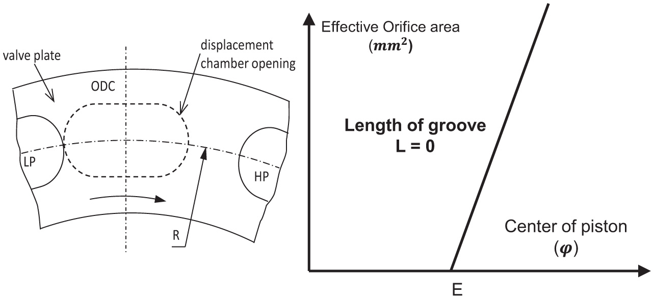
Figure A1 Groove area for ideal timing.
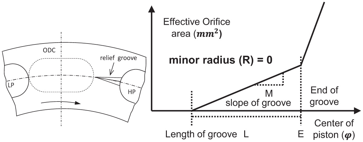
Figure A2 Groove area for linear relief groove.
References
Blum, C. and Roli, A. 2003. Metaheuristics in combinatorial optimization: Overview and conceptual comparison. ACM Computing Surveys, pp. 268–308.
Deb, K., Pratap, A., Agarwal, S. and Meyarivan, T. 2002. A fast and elitist Multiobjective genetic Algorithm: NSGA-II. IEEE Transactions on evolutionary Computation, 6(2).
Edge, K.A. 1999. Designing quieter hydraulic systems – some recent developments and contributions. In Fourth JHPS International Symposium on FLuid Power. Tokyo, Japan, 1999.
Edge, K.A. and Liu, Y. 1989. Reduction of piston pump pressure ripple. In Second International Conference on Fluid Power Transmission and Control. China, 1989.
Frosina, E., Marinaro, G., Senatore, A. and Pavanetto, M. 2018. Effects of PCFV and Pre-Compression Groove on the Flow Ripple Reduction in Axial Piston Pumps. 2018 Global Fluid Power Society PhD Symposium, GFPS 2018, (July).
Harrison, A.M. 1997. Reduction of Axial Piston Pump Pressure Ripples. PhD Thesis, University of Bath, UK.
Helgestad, B.O., Foster, K. and Bannister, F.K. 1974. Pressure transient in an axial piston hydraulic pump. In Institution of Mechanical Engineers., 1974.
Ivantysn, J. and Ivantysynova, M. 2001. Hydrostatic Pumps and Motor, Principles, Designs, Performance, Modeling, Analysis, Control and Testing. New Delhi: Academic Books International.
Ivantysynova, M., Huang, C. and Christiansen, S.K. 2004. Computer Aided Valve Plate Design – An Effective Way to Reduce Noise. In Proceedings of the SAE Commercial Vehicle Engineering Congress & Exhibition. Chicago, IL USA, 2004. SAE Technical Paper.
Johansson, A. 2005. Design Principles for Noise Reduction in Hydraulic Piston Pumps – Simulation, Optmization and Experimental Verification. PhD Thesis, Linkoping University, Sweden.
Kim, T., Kalbfleisch, P. and Ivantysynova, M. 2014. The effect of cross porting on derived displacement volume. International Journal of Fluid Power, 15(2), Taylor & Francis. pp. 77–85.
Klop, R.J. 2010. Investigation of Hydraulic Transmisson Noise Sources. PhD thesis, Purdue University.
Lasaar, R. and Invantysynova, M. 2004. An investigation into micro- and macrogeometric design of piston/cylinder assembly of swash plate machines. International Journal of Fluid Power, (1). pp. 23–36.
Palmberg, J.O. 1989. Modelling of flow ripple from fluid power piston pumps. In 2nd Bath International Power Workshop., 1989. Univeristy of Bath, UK.
Pettersson, M.E. 1995. Design of Fluid Power Piston Pumps: with Special Reference to Noise Reduction. Universitetet i Linköping.
Pettersson, M., Weddfelt, K. and Palmberg, J.O. 1991. Methods of reducing flow ripple from fluid power piston pumps – a theoretical approach. In SAE International Off-highway and Powerplant Congress. Milwaukee, USA, 1991.
Petzold, L. 1983.Automatic Selection of methods for solving stiff and nonstiff systems of ordinary differential equations. SIAM Journal on Scientific and Statistical Computing, 4(1).
Schleihs, Christian, Viennet, Emmanuel, Deeken, Michael, Ding, Hui, Xia, Yanjun, Lowry, Samuel and Murrenhoff, Hubertus 2014. 3D-CFD simulation of an axial piston displacement unit. Internationales Fluidtechnisches Kolloquium.
Seeniraj, G.K. 2009. Model based optimization of axial piston machines focusing on noise and efficiency. PhD Thesis, Purdue University.
Wieczorek, U. and Ivatysynova, M. 2002. Computer aided optimization of bearing and sealing gaps in hydrostatic machines – the simulation tool CASPAR. International Journal of Fluid Power, 3(1). pp. 7–20.
Yamauchi, K. and Yamamoto, T. 1976. Noises gernated by hraulic pumps and their control method. Mitsubshi Techical Review, 13(1).
Zhang, B., Xu, B., Xia, C. and Yang, H. 2009. Modeling and Simulation on Axial Piston Pump Based on Virtual Prototype Technology. Chinese Journal of Mechanical Engineering, 22(1), Editorial Office Chinese Journal Mechanical Engineering. pp. 84–90.
Zitzler, E., Deb, K. and Thiele, L. 2000. Comparison of Multiobjective Evolutionary Algorithms: Empirical Results. Evolutionary Computation, 8(2). pp. 173–95.
Biographies
Paul Kalbfleisch Born on November 20th 1988 in Louisville, Kentucky (USA). He received his B.S degree in Engineering in Acoustics from Purdue University in 2011, a M.S.E degree in Mechanical Engineering at Purdue University in 2015 and currently a Phd student. His main research interests are Noise, Vibration, and Harshness modeling and design of hydraulic pumps/motors and transmissions.
Monika Ivantysynova Born on December 11th 1955 in Polenz (Germany). She received her MSc. Degree in Mechanical Engineering and her PhD. Degree in Fluid Power from the Slovak Technical University of Bratislava, Czechoslovakia. After 7 years in fluid power industry she returned to university. In April 1996 she received a Professorship in fluid power & control at the University of Duisburg (Germany). From 1999 until August 2004 she was Professor of Mechatronic Systems at the Technical University of Hamburg-Harburg. Since August 2004 she is Professor at Purdue University, USA. Her main research areas are energy saving actuator technology and model based optimization of displacement machines as well as modelling, simulation and testing of fluid power systems. Besides the book “Hydrostatic Pumps and Motors” published in German and English, she has published more than 80 papers in technical journals and at international conferences. Monika passed away August 11th 2018.
International Journal of Fluid Power, Vol. 20_2, 177–208.
doi: 10.13052/ijfp1439-9776.2022
© 2019 River Publishers