An Electrohydraulic Pressure Compensation Control System for an Automotive Vane Pump Application
Ryan P. Jenkins* and Monika Ivantysynova
Maha Fluid Power Research Center, School of Mechanical Engineering, Purdue University, 585 Purdue Mall, West Lafayette, Indiana 47907, USA
E-mail: jenkins.r89@gmail.com
* Corresponding Author
Received 13 February 2019; Accepted 05 March 2020; Publication 20 March 2020
Abstract
Pressure compensated vane pumps are an excellent solution for supplying hydraulic power with minimal waste in many automotive applications. An electrohydraulic pressure compensation control system for an automatic transmission supply that promises improved pressure response times over the baseline architecture is discussed. Suggested valve specifications are determined through calculations based on available data and refined via a validated simulation model of the proposed system. Two controller designs are formulated and compared: a basic PI control law and a cascaded model following controller including a nonlinear feedback linearization component. Simulations of the proposed system for a given duty cycle reveal that the nonlinear controller provides only minor improvements over a basic PI control law and is thus not an economical solution.
Keywords: Vane pump, electrohydraulic pressure compensation, automotive transmission supply, PID control, nonlinear control.
1 Introduction
Variable displacement vane pumps (VDVP) are well suited to the task of supplying hydraulic power in many automotive applications as they are easily configurable as a pressure compensated system which reduces power loss at high engine speeds. Pump displacement control in these situations can be effected directly via a bias spring and internal routing of the pump outlet pressure [1, 2]. Valves can also be used to regulate the pressure acting against the spring thereby controlling the pump displacement [3, 4].
An advantage of using valves to control the pump displacement is that a variable pressure compensation set point (i.e. the reference outlet pressure) can be used to better meet pressure requirements of distinct load functions. For example, the automatic transmission oil supply system treated in [3] must maintain a nearly constant low pressure to satisfy cooling and lubrication demands while providing a high pressure during shifting events. At each of these two pressure levels, the traditional pressure compensation function of regulating the pump displacement to match the flow requirement of the load must still be met. This may be done with a solenoid-valve-controlled pilot pressure acting on a conventional regulation valve as in the baseline system considered here and treated in [3].
This baseline control system architecture, depicted on the left-hand side of Figure 1, has several drawbacks including a 190 ms response time and an unstable zero in the transfer function from the pump outlet pressure to the regulation valve’s (V1) flow output. The primary reason for this poor performance is the solenoid valve V3 which contributes a low bandwidth of 1.84 Hz and a 30 ms time delay along with other nonlinearities such as hysteresis and sensitivity to temperature [3, 5]. The unstable zero, on the other hand, arises from the architecture itself with the pilot line feedback loop containing V3 supplied by V2.
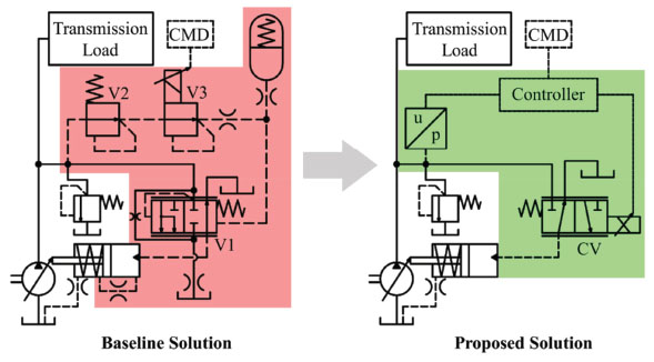
Figure 1 Proposed electrohydraulic architecture compared with the current semi-active pressure compensation control system for an automotive application taken as a baseline.
To address these limitations, the proposed electrohydraulic control system treated in this article was introduced in [3] and is depicted on the right-hand side of Figure 1. This control system consists of a 3/2 proportional directional control valve (CV), a miniature pressure transducer near the pump outlet, and a microcontroller to both process the transducer signal and generate a proportional command to control the valve. The introduction to this proposed system architecture provided in [3] only includes a brief description of its design and results from initial proof of concept simulations and measurements only considering a PI controller.
This paper, on the other hand, goes more in depth and evaluates this proposed design by first specifying control valve requirements before demonstrating its performance with a validated simulation model. The formulation, and subsequent comparison, of two pressure compensation controller designs is presented. These designs can be categorized as a simple PI approach and a cascaded nonlinear approach. Comparing these options provides a valuable initial framework for a cost/benefit analysis of electrifying automotive oil supply systems with variable displacement vane pumps in this fashion.
Figure 2 gives an example of one of these pumps which falls under the classification of pivoting-cam type single-stroke variable displacement vane pumps [6]. Other common vane pump designs used in automotive applications include sliding-cam type variable displacement units [7] and some double stroke fixed displacement units [8] although other designs have been explored [9]. While the pivoting-cam type pump in the case study system is only one pump configuration, the results here can be applied to other pump configurations for other automotive applications.
2 State of the Art
Currently, there is no – or at least very little – literature available treating the electrohydraulic control of a variable displacement vane pump (VDVP) in a pressure compensated automotive application specifically. Considerably more literature is available for electrohydraulic pump displacement control in high power pressure controlled applications which primarily use swashplate-type axial piston pumps [10–12]. While many of the techniques used in these high power applications have not been applied to vane pumps, several authors have nevertheless investigated a few techniques for similar electrohydraulic control system designs for vane pumps in low pressure applications.
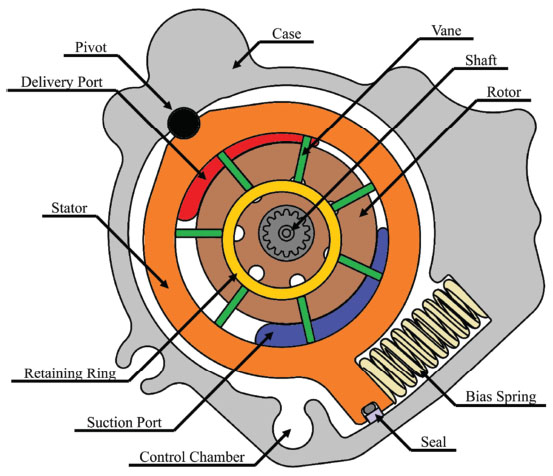
Figure 2 Cross-sectional schematic of the 25cc/rev case study vane pump for an automotive transmission application.
In 1997, Thompson and Kremer presented the development of an optimal feedback controller design using the Quantitative Feedback Theory technique [13]. Their work was based on a linearized parametrically uncertain model. While the problem statement in [13] indicates a similar setup and control task (i.e. line pressure regulation), no results are shown to indicate the achieved, or predicted, performance.
Later, Köster and Fidlin presented a nonlinear volume flow control law for a VDVP in an automotive transmission application [14]. They employ input-output linearization to develop an observer-based state-space control approach and also present an inversion-based feedforward controller design. Both controllers result in good displacement control, but their application to a pressure compensation task is not demonstrated.
The notion, however, of using a pump with electrohydraulic displacement control as a pressure controlled supply is not new as it is commonly done with the primary unit in secondary controlled hydraulic circuits (see [15, 16] for an example). Considering this, there is a wealth of literature that deals in some respect with the topic of electrohydraulic pressure compensation that may be referred to in selecting a control methodology. However, many of these approaches (including that introduced in [15]) may not be feasible for an automotive application in light of a cost/benefit analysis.
Regardless of the chosen approach, development and virtual evaluation of the controller relies on a validated system model capable of generating representative dynamics and the internal forces that must be overcome by the control system to effect displacement changes. The work presented here is based on a lumped parameter model of this type describing the case study VDVP previously developed by the author and discussed in [17].
3 Control Valve Requirements
Determining appropriate requirements on the control valve characteristics begins with an understanding of the dynamic flow demands and desired system response times for the case study application. In this case study, the 25 cc/rev pump is chain-driven by the engine crankshaft and supplies hydraulic power to the transmission required to actuate clutches as well as lubricate and cool the gears. Figure 3 provides measured pump speeds and system pressures from an example duty cycle for the case study system where the vehicle accelerates from stand-still to a moderate speed. As the flow demand and pump displacements were not measured in the case study vehicle, the pump displacement was estimated for this cycle using the validated lumped parameter model presented in [17].
With this information, the pressure-flow characteristics for the control valve in the proposed system architecture can be determined by calculating the flow rate required to effect the desired displacement change in a given time interval and analysing the differential pressure across the valve during that interval. If this flow is denoted by Qβ and the corresponding differential pressure by Δp, then the flow gain Kv is given by (1).
| (1) |
This flow gain may be calculated for a given event such as the step increase at 10 s in Figure 3 (what was done in [3]). While the value of Kv determined from this event may be adequate to satisfy other events, it is better to calculate an instantaneous Δp and Qβ using the simulation model and the definitions (2) through (4) for a typical duty cycle.
| (2) |
| (3) |
| (4) |
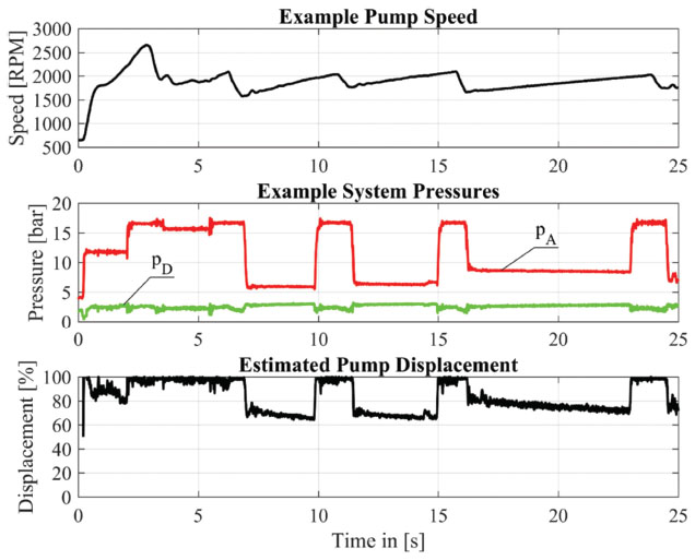
Figure 3 Example pump speeds and system pressures along with estimated pump displacements calculated using a validated lumped parameter model.
In these expressions, β refers to the pump displacement, VD to the control chamber volume, pA to the main line pressure, pT to the reservoir pressure, M1 to the internal moments acting on the stator, k to the bias spring rate, and CS to the lumped stator friction coefficient. The parameter τRC is for converting the control chamber pressure pD into an applied moment acting on the stator and is the sum of the product of two projected areas orthogonal with each other and the distance between their centroids and the pivot pin centreline. The other parameters are geometric constants such as moment arm lengths (bL) and spring lengths (lf and l0) required for calculating the spring’s compressed length (see [17] for more details).
The pD calculated by (4) estimates the required pressure level for the proposed architecture, neglecting the impact of the stator inertia, even though a measurement of the control pressure for the cycle in Figure 3 is available because this measurement is affected by the increased control chamber leakage and line capacitance of the baseline system depicted in Figure 1.
Figure 4 illustrates the varying requirement on Kv for a brief segment of the cycle containing the maximum value. This corresponds to a step in the required system pressure and flow supplied by the pump in anticipation of a transmission shifting event. Rounding this maximum value up to a flow gain of 5 [L/min]/bar means that the control valve flows required by the duty cycle depicted in Figure 3 can be provided with a small safety margin. Since this selection corresponds to a shifting event and it is unknown how many clutches were actuated in this instance, the highlighted moment in Figure 4 may or may not represent the most demanding requirement. It is nevertheless a valuable guidepost in selecting an appropriate control valve.
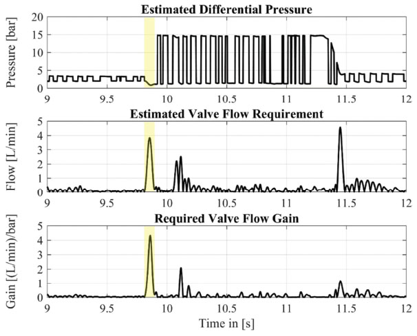
Figure 4 Estimate of the maximum required valve flow gain during the duty cycle depicted in Figure 3.
While the flow gain is certainly an important defining characteristic of the control valve, it is not the only parameter that should be considered. In order to satisfy the required dynamic performance of the system, the control valve should also possess a satisfactory frequency response which will be characterized here by its bandwidth. The assumption is that higher bandwidths will translate into faster changes in the spool position resulting in a tighter control of the control chamber flow. Tighter flow control means tighter pump displacement control and, ultimately, a better possible pressure compensation behaviour.
Estimating the required valve bandwidth, however, can be difficult. Analysing the step response of the baseline system during the highlighted event in Figure 4 reveals a displacement rise time of 100 ms and a pressure rise time of 190 ms. Since the rise in the reference pressure profile during this event occurs over 40 ms, it stands to reason that a target rise time for the displacement might be 20 ms. Assuming that, due to the stiffness of the oil within the control chamber, the valve spool must therefore exhibit a similar 10% to 90% rise time tr, (5) can be used to estimate the required bandwidth fBW in Hertz.
| (5) |
Performing this calculation results in a bandwidth of 17.5 Hz. Direct drive valves are capable of attaining these bandwidths for a relatively low cost [18], so a selection of a 20 Hz at ±100% stroke can reasonably be taken as a starting point for the valve specifications. These valve specifications (5 [L/min]/bar and 20 Hz at ±100% stroke) could be iteratively refined through simulations and physical experimentation, but will be assumed as the nominal valve specifications for this research.
4 Simulation Model
Implementing a control valve with these suggested specifications in simulation allows for an evaluation of the proposed system for comparison with the baseline architecture. In this context, and assuming a simple PI controller, the proposed system model can then be expressed by the block diagram given in Figure 5.
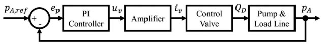
Figure 5 Block diagram giving the general structure of the simulation model describing the proposed system with a basic PI control law.
The electromechanical behaviour of the control valve, neglecting amplifier dynamics, can be expressed through the use of a standard second order LTI transfer function (6) which expresses the normalized spool position xv response to a proportional voltage command uv.
| (6) |
Where ωBW is fBW expressed in rad/s and ζv is the damping ratio set to a value of 0.7. This xv is used to determine control valve flow QD when combined with Kv in the orifice equation for turbulent flow with appropriate differential pressures as in (7), where ρf represents the density of the working fluid. This approach is similar to the one in [14].
| (7) |
This flow QD is converted into the main system pressure pA by solving the system of equations described by (8) through (10). In these equations, β is the angular eccentricity of the vane pump’s pivoting cam and Kf is the effective bulk modulus of the working fluid. Meanwhile, (10) approximates the transmission as a general impedance model resistance.
| (8) |
| (9) |
| (10) |
The terms QA and M1 here represent the effective flow output and internal moments of the pump, respectively, and come from the displacement chamber module presented in [17] which simulates the rotating group. These quantities, therefore, are essentially nonlinear functions of the pump displacement β, line pressure pA, and pump speed n. The term Mst in (9) is also a nonlinear function of β that introduces some damping and a stiff spring force when the stator reaches the limits of its motion as defined by the pump geometry.
It should be noted that while (10) is a simplistic representation of the automatic transmission load in the case study application, a more realistic model as in [19, 20] is outside the scope of this work. The objective of this research is merely to present an electrohydraulic pressure compensated pump architecture suitable for an automotive transmission application and not provide a complete transmission model.
5 Basic PI Control Law
As the most commonly used controller design, proportional-integral-derivative (PID) controllers in various forms solve between 90–95% of all control problems [21]. Due to the fact that each of the three terms in a general PID controller has a different interpretation, and therefore function, an initial part of the design procedure includes the selection of a proper controller structure for the application at hand [22]. For the automatic transmission application studied here, a relatively first order process dynamics and a line pressure set point that is normally constant and low with periodic steps up to a constant high value preclude the use of a derivative term. In order to reduce steady-state errors and assure that sufficient pressures are maintained for proper lubrication and clutch operation, an integral term is desirable. For these reasons, a standard PI controller as given by (11) was selected.
| (11) |
Where ep is the difference between the set point pA,ref and the measured pA as defined in Figure 5. The gains in (11) were found to result in a satisfactory response in simulation after some manual tuning as there are not readily available PID gain formulas for pump controlled pressure applications as there are for valve controlled ones [23]. A starting point for this tuning procedure can be easily found using a simplified form of the model presented in the previous section. Assuming a restrictive nominal differential pressure, QD can be approximated by (12). Assuming the control chamber pressure dynamics to be sufficiently fast and the resulting moment on the stator perfectly balances the internal displacement chamber moments and bias spring preload, QD can be subsequently thought of as a velocity input to the stator dynamics equation and (9) can be rewritten as (13).
| (12) |
| (13) |
| (14) |
Equation (14) completes this simplified pump model by assuming QA is close to the theoretical volumetric flowrate of the pump for a mean value of the speed during the duty cycle in Figure 3 and can therefore be represented by the product of the speed, stator eccentricity, and a constant c. Combining (6) with (12) through (14) approximates the plant portion of the system as diagrammed in Figure 5.
This new representation can then be analysed in MATLAB using automated tuning methods find control gains that result in a robust response time less than 20 ms. Despite using such a simplified plant model, this approach generates PI controller gains that give good results and only need minor fine tuning to arrive at (11).
6 Experimental Validation
In order to validate the control valve model, the experimental setup introduced in [24] was modified according to the proposed electrohydraulic control system architecture with a custom plate to adapt an available servo-valve to the existing pump/valve block interface. A permanent magnet linear force motor actuates the spool of the implemented direct drive valve which was sized for a 10 L/min flowrate at a differential pressure of 35 bar per metering edge and exhibited a 60 Hz frequency response at ±50% stroke.
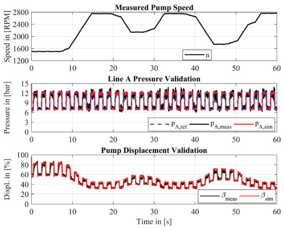
Figure 6 Comparison of experimental data and simulated results for the PI controlled proposed electrohydraulic pressure compensated pump system to highlight the representative model agreement and responsiveness of the system.
While the flow gain of the implemented valve is suboptimal for this application and results in flow saturation of the valve at such low differential pressures, the frequency response exceeds the required specifications given earlier. Fortunately, with reduced leakages, the control chamber pressure dynamics are stiff enough that smaller flows can now produce changes in the displacement more easily. This effect is sufficient enough that proper pressure compensation behaviour is observed in the measured results given by Figure 6 (black lines) when the PI control law (11) is used.
These measurements not only provide a physical proof of concept that the proposed system is a capable of satisfying the demands of the case study application, but also indicate the validity of the simulation model when two small modifications to the model are made. First, the valve specifications of the implemented valve are substituted for the proposed ones discussed in Section 3 of this paper. Second, the coefficients used in (10) were tuned using additional measurements to characterize the experimental loading conditions.
Since the transmission load model can be handled separately from the supply pump model, Figure 6 is therefore sufficient to conclude that the control valve and pump models discussed in this work may be used to predict the performance of the proposed system over the case study duty cycle assuming the suggested valve characteristics. A comparison of the predicted performance with the baseline performance (see [3] for an in depth discussion of the baseline control system for the case study application) will therefore be presented in Section 8 of this work.
7 Cascaded Nonlinear Controller
While PI controllers can be used to satisfactorily solve many control problems, they are also frequently used as a first approach when designing a feedback controller as the “bread and butter” of automatic control [22]. Advanced controller designs of many varieties have been developed over the past few decades and may be applied to numerous applications [25]. Many of these approaches have been previously applied to fluid power systems and automotive applications to accomplish various tasks. Thus, the focus here is only to provide an alternate controller design that may be compared with the basic PI law as a way to cast the framework for a brief cost/benefit analysis within the context of an automotive application. Figure 7 diagrams the system with this alternate controller.
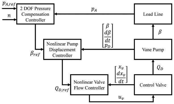
Figure 7 Block diagram of the proposed system simulation model with the cascaded nonlinear controller.
As Figure 7 indicates, there are three levels of control in this cascaded structure. At the highest level, a two degree of freedom pressure compensation law given by (15) outputs a desired pump displacement for a given pA,ref, pa, and n. The feedforward portion βff of (15) is based on a model inversion gained by inverting (10) and dividing the result by the theoretical pump flow as given by (16). The feedback portion βfb, (17), combines a low-pass filter and a PI law tuned to reduce remaining steady-state errors after application of the feedforward term that are due to modelling error.
| (15) |
| (16) |
| (17) |
The two nonlinear controller blocks depicted in Figure 7 are similar in construction, but different in purpose. In both cases the controller is comprised of a local state feedback control law derived using the feedback linearization approach available in Chapter 46 of [25] (utilizing Lie derivatives which can be thought of as a type of partial derivative) and a model following control law. The Lie derivatives of the two nonlinear state space systems are not included here for the sake of brevity, but both are of the so called ‘standard form’ in [25] and lead to the following observations.
- The relative degree of the vane pump system is three when the state vector is described by the pump feedback line in Figure 7, β is the output, and the model described in Section 4 of this work is used to describe the three state equations. This means that the system can be transformed into a system that is linear and controllable by means of a local static state feedback [25] given by (18) in terms of an artificial input νβ and the Lie derivatives and .
- The term normally included in (18) corresponding to the partial derivative of with respect to pD was neglected as initial simulations proved that it cancelled out a stabilizing term in the third state equation of the vane pump system.
- The relative degree of the control valve system is two when the state vector is described by the valve feedback line in Figure 7 with the state equations given by the relationship contained in (6) and the output is QD as given by (7). The case structure of (7) was removed by combining the two flow cases using appropriate sign function representations of the Heaviside step function. For simplicity, the derivative of the sign function was assumed to be zero everywhere. As before, the relative degree here indicates that a local static state feedback, (19), with an artificial input νQ results in a linear and controllable system.
| (18) |
| (19) |
The artificial inputs in (18) and (19) are given by the model following control laws (20) and (21), respectively, for errors defined by (22) and (23). The gains γβ and γQ in (20) and (21) were set to 3207T and 80π for this application and were tuned using simulations of the vane pump and control valve subsystems with other parameters, such as the pump speed, held constant and produced good tracking results.
| (20) |
| (21) |
| (22) |
| (23) |
The nonlinear controller described in this section is similar to the inversion-based feedforward controller design presented in [14] and is thus not a new concept within automotive transmission research. As previously stated, the purpose of this work is to provide a single alternative to PI control and is therefore sufficient for the present discussion, as the results in the following section will show, despite any limitations it may have. It could be made more robust by augmenting the model following component with integrator action or a fast-switching sliding mode term, but that will be left to future work.
8 Predicted Performance
Figure 8 compares the predicted pressure response of the proposed system using both PI control and the cascaded nonlinear controller with the measured response taken from vehicle data where the baseline case study system was installed. As this figure illustrates, the proposed electrohydraulic pressure compensation control system satisfies the specific requirements of the case study application in that it maintains constant mean pressure levels despite variable engine speeds and responds quickly to changes in the reference.
However, it is clear that there is still room for improvement as the PI controller results exhibit large pressure oscillations. This is largely due to chattering in the control signal that arises from trying to damp out existing, and inherent, pump pressure fluctuations. Improving the robustness and disturbance rejection properties of the implemented controller, along with considering more realistic transmission load dynamics, will only help the proposed system in this respect. The nonlinear controller results are better as it is capable of cancelling out more of these oscillations, even with a limited valve bandwidth, through its feedback linearization component.
The ability of the controller (nonlinear or not) to cancel out oscillations improves with higher control valve bandwidths. Figure 9 provides predicted responses for the proposed system with identical controllers and a 60 Hz control valve with the suggested flow gain for comparing to Figure 8. As can be clearly seen, the higher valve bandwidth coupled with the PI controller significantly attenuates the pressure oscillations in the system. Meanwhile, fluctuations with the nonlinear controller increase. This indicates further tuning of the model following gains is required.
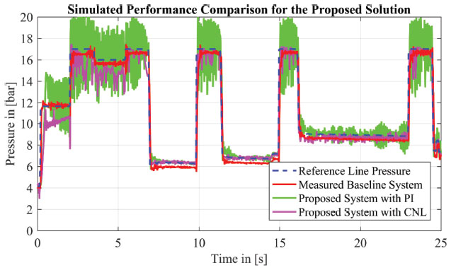
Figure 8 Comparison of the predicted pressure responses for the proposed system employing both the basic PI controller and the cascaded nonlinear (CNL) controller with the measured baseline response for the duty cycle shown in Figure 3.
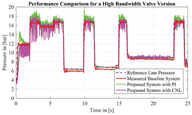
Figure 9 Comparison of the predicted performance with the baseline system similar to Figure 8 but considering a 60 Hz at ±100% control valve.
For either controller approach, additional development efforts of this nature will clearly lead to improved performance. As the work presented here is intended more as a proof of concept to highlight the potential of an electrohydraulic pressure compensation control system for an automotive transmission application than a thorough treatise on the controller development as a precursor to actual implementation, no additional development will be included. However, looking closer and past the depicted pressure oscillations gives another measure of the proposed system architecture’s potential.
Figure 10 shows a single 2.5 s step event from the duty cycle to allow for a more direct comparison of the resulting performance with both controllers alongside the baseline performance for context. As Figure 10 shows, the proposed system responds more quickly to a reference step input. In fact, the proposed system, with the suggested 20 Hz valve, offers a 47% reduction in the 10% to 90% rise time over the baseline system with the PI controller and a 58% reduction with the cascaded nonlinear controller. Considering the 60 Hz valve and the same controllers, as in Figure 10, results in 69% and 77% reductions, respectively. Surprisingly and despite a sub-optimal flow gain on the implemented control valve, the measured rise time with PI control in the experimental setup exceeded even these predictions with almost a 90% reduction (see also [3]).
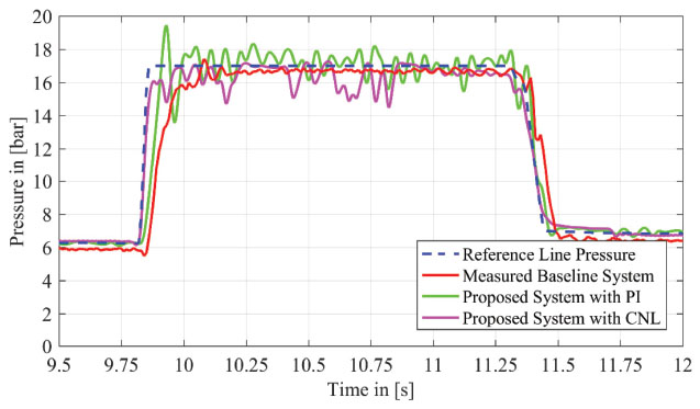
Figure 10 Contracted timescale view of the results depicted in Figure 9 to allow for a more direct comparison of the step response.
9 Summary
While response time is only one metric of the system performance, it does illustrate the potential of the proposed system in an automotive application. As the results in the previous section convey, significant improvements in terms of the pressure response times are possible with a simple PI controller and an appropriate selection of a 3/2 proportional control valve. This configuration only requires the addition of a single pressure transducer to monitor the outlet pressure of the pump and is thus more economical as a solution than implementing a more complex controller which only gives marginal improvements (over the PI) and requires additional sensors and/or nonlinear observers.
Selection of an appropriate valve is therefore of paramount significance. Calculations based on available data can aid in determining an appropriate flow gain and simulations can help to determine a target valve bandwidth to adequately meet a given duty cycle. For the case study application, it is suggested that the valve be sized for a flowrate of 5 L/min at a 5 bar differential pressure per metering edge and possess a 20 Hz bandwidth at ±100% stroke and 60 Hz bandwidth at ±40% stroke. This can be accomplished using currently available permanent magnet linear force motors [26] and an appropriate spool design.
Acknowledgements
The primary author would like to acknowledge Prof. Andrea Vacca for his support and advice in the preparation of this article which occurred after the passing of Prof. Monika Ivantysynova during the final stages of the research discussed here.
References
[1] B. Geist, W. Resh, K. Aluru, ‘Calibrating an Adaptive Pivoting Vane Pump to Deliver a Stepped Pressure Profile’, SAE Technical Paper 2013-01-1729, 2013.
[2] T. Arata, N. Novi, K. Ariga, A. Yamashita, G. Armenio, ‘Development of a Two-Stage Variable Displacement Vane Oil Pump’, SAE Technical Paper 2012-01-0408, 2012.
[3] R. Jenkins, M. Ivantysynova, ‘An Empirically Derived Pressure Compensation Control System for a Variable Displacement Vane Pump’, Proceedings of the 2018 Bath/ASME Symposium on Fluid Power and Motion Control, Bath, United Kingdom, 2018.
[4] M. Rundo, ‘Piloted Displacement Controls for ICE Lubricating Vane Pumps’, SAE International Journal of Fuels and Lubricants, Vol. 2, No. 2, pp. 179–184, 2009.
[5] Z. Sun, K. Hebbale, ‘Challenges and Opportunities in Automotive Transmission Control’, Proceedings of the 2005 American Control Conference, pp. 3284–3289, Portland, Oregon, 2005
[6] J. Ivantysyn, M. Ivantysynova, ‘Hydrostatic Pumps and Motors’, New Delhi: Academic Books International, 2001.
[7] M. Rundo, G. Altare, ‘Lumped Parameter and Three-Dimensional Computational Fluid Dynamics Simulation of a Variable Displacement Vane Pump for Engine Lubrication’, Journal of Fluids Engineering, Vol. 140, No. 6, pp. 061101-061101-9, 2018.
[8] A. Giuffrida, R. Lanzafame, ‘Cam Shape and Theoretical Flow Rate in Balanced Vane Pumps’, Mechanism and Machine Theory, Vol. 40, No. 3, pp. 353–369, 2005.
[9] M. Rundo, N. Nervegna, ‘Lubrication Pumps for Internal Combustion Engines: A Review’, International Journal of Fluid Power, Vol. 16, No. 2, pp. 59–74, 2015.
[10] J. Grabbel, M. Ivantysynova, ‘An Investigation of Swash Plate Control Concepts for Displacement Controlled Actuators’, International Journal of Fluid Power, Vol. 6, No. 2, pp. 19–36, 2005.
[11] C. Williamson, S. Lee, M. Ivantysynova, ‘Active Vibration Damping for an Off-Road Vehicle with Displacement Controlled Actuators’, International Journal of Fluid Power, Vol. 10, No. 3, pp. 5–16, 2009.
[12] M. Bahr Khalil, V. Yurkevich, J. Svoboda, R. Bhat, ‘Implementation of Single Feedback Control Loop for Constant Power Regulated Swash Plate Axial Piston Pumps’, International Journal of Fluid Power, Vol. 3, No. 3, pp. 27–36, 2002.
[13] D. Thompson, G. Kremer, ‘Quantitative Feedback Design for a Variable-Displacement Hydraulic Vane Pump’, Proceedings of the 1997 American Control Conference, Albuquerque, New Mexico, 1997.
[14] M. Köster, A. Fidlin, ‘Variable Displacement Vane Pump, Part II: Nonlinear Volume Flow Control’, Nonlinear Dynamics, Vol. 90, No. 2, pp. 1091–1103, 2017.
[15] E. Busquets, M. Ivantysynova, ‘A Robust Multi-Input Multi-Output Control Strategy for the Secondary Controlled Hydraulic Hybrid Swing of a Compact Excavator with Variable Accumulator Pressure’, Proceedings of the 2014 Bath/ASME Symposium on Fluid Power & Motion Control, Bath, United Kingdom, 2014.
[16] E. Busquets, M. Ivantysynova, ‘Adaptive Robust Motion Control of an Excavator Hydraulic Hybrid Swing Drive’, SAE International Journal of Commercial Vehicles, Vol. 8, No. 2, pp. 568–582, 2015.
[17] R. Jenkins, M. Ivantysynova, ‘A Lumped Parameter Vane Pump Model for System Stability Analysis’, International Journal of Hydromechatronics, Vol. 1, No. 4, pp. 361–383, 2018.
[18] A. Plummer, ‘Electrohydraulic servovalves – past, present, and future’, Proceedings of the 10th IFK International Conference on Fluid Power, Dresden, Germany, 2016.
[19] A. Karmel, ‘Dynamic Modeling and Analysis of the Hydraulic System of Automotive Automatic Transmissions’, American Control Conference, Seattle, Washington, 1986.
[20] G. Lucente, M. Montanari, C. Rossi, ‘Modelling of an Automated Manual Transmission System’, Mechatronics, Vol. 17, No. 2–3, pp. 73–91, 2007.
[21] K. Åström, T. Hägglund, ‘PID Control’, The Control Handbook: Control System Fundamentals, 2nd edition, CRC Press, Edited by W. Levine, 2010.
[22] K. Åström, T. Hägglund, ‘The Future of PID Control’, IFAC Proceedings Volumes, Vol. 33, No. 4, pp. 19–30, 2000.
[23] M. Liermann, ‘PID Tuning Rule for Pressure Control Applications’, International Journal of Fluid Power, Vol. 14, No. 1, pp. 7–15, 2013.
[24] R. Jenkins, M. Ivantysynova, ‘Investigation of Instability of a Pressure Compensated Vane Pump’, Proceedings of the 9th FPNI Ph.D. Symposium on Fluid Power, Florianópolis, Brazil, 2016.
[25] The Control Systems Handbook: Control System Advanced Methods, 2nd Edition, CRC Press, Edited by W. Levine, 2010.
[26] Moog.com, ‘Direct Drive Servovalves D633/D634’, [online] Available at: http://www.moog.com/literature/ICD/Moog-Valves-D633_D634-Catalog-en.pdf [Accessed 5 Feb. 2019], 2009.
Biographies

Ryan P. Jenkins was born on December 16, 1989 in Provo, Utah (USA). He received his B.S degree in Mechanical Engineering from Brigham Young University in 2014. He worked as a PhD student under the direction of Monika Ivantysynova with a focus on the modeling, analysis, and control of fluid power systems at Purdue University’s Maha Fluid Power Research Center. He has worked on several projects dealing with automotive applications of fluid power technologies and defended his thesis in January 2019. He now works as a hydraulics engineer overseeing advanced engineering development and simulations for hydraulic systems and components at CNH Industrial with a focus on developing subsystems for use in autonomous agricultural machinery.

Monika Ivantysynova was born on December 11th 1955 in Polenz (Germany). She received her MSc. Degree in Mechanical Engineering and her PhD. Degree in Fluid Power from the Slovak Technical University of Bratislava, Czechoslovakia. After 7 years in fluid power industry she returned to university. In April 1996 she received a Professorship in fluid power & control at the University of Duisburg (Germany). From 1999 until August 2004 she was Professor of Mechatronic Systems at the Technical University of Hamburg, Harburg. Since August 2004 she is Professor at Purdue University, USA. Her main research areas are energy saving actuator technology and model based optimization of displacement machines as well as modelling, simulation and testing of fluid power systems. Besides the book “Hydrostatic Pumps and Motors” published in German and English, she has published more than 80 papers in technical journals and at international conferences. Monika passed away August 11th 2018.
International Journal of Fluid Power, Vol. 20_3, 353–374.
doi: 10.13052/ijfp1439-9776.2034
© 2020 River Publishers