A Note on Leakage Jet Forces: Application in the Modelling of Digital Twins of Hydraulic Valves
Zoufiné Lauer-Baré1,*, Erich Gaertig1, Johannes Krebs1, Christian Arndt1, Christian Sleziona1 and André Gensel2
1Simulation Department, Hilite Germany GmbH, Nürtingen, Germany
2Testing Department, Hilite Germany GmbH, Nürtingen, Germany
E-mail: zoufine.lauer-bare@hilite.com
*Corresponding Author
Received 25 September 2020; Accepted 23 February 2021; Publication 27 April 2021
Abstract
The proper modelling of fluid flow through annular gaps is of great interest in leakage calculations for many applications in fluid power technology. However, while detailed numerical simulations are certainly possible, they are very time consuming, in various cases prone to numerical instabilities and may not even include all physically relevant effects. This is an issue especially in system simulations, where a large set of computations is needed in order to prepare the lookup-tables for the required input fields. In this work, an analytical approximation for the shear force, which is induced by viscous flow between two eccentric cylinders, is presented. This relation, and its derivation, mimics and enhances the well-known Piercy-relation for the corresponding volume flow that is utilized in state-of-the-art system simulation tools. To determine its range of validity, the analytical relation for the shear force is compared to 3D-simulations. Additionally, an application of this approximation for creating digital twins of hydraulic valves is also discussed in this work.
Keywords: Annular flow, flow force, leakage, eccentric annulus, valve, digital twin.
1 Introduction
The flow through annular gaps is of great interest in all areas of fluid power technology, see for instance [10, 5, 16], where the flow is caused by internal leakage of valves. Other applications of this kind can be found in petroleum engineering; see e.g. [6, 9], or in the nuclear sciences (see [1]) in the context of two-phase flows. It is also utilized for hemodynamic studies in medical appliances; see for instance [24] for a study of the blood flow in arteries. In general, the fluid flow through an annular domain between two cylinders is viscous and induces shear forces (leakage jet forces, viscous flow forces) that act upon the surface of the inner cylinder; see [21] or [4]. These forces can either be computed numerically, which requires detailed meshing and is time consuming, or in certain simple cases analytically, which then yield results that are as accurate as equivalent numerical findings from full 3D-simulations.
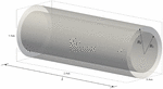
For further reference and as the general setup for the following discussion, Figure 1 shows two concentric cylinders of length , inner radius and outer radius , oriented along the positive -axis. The annular flow domain mentioned above is contained in the region between these two cylinders.
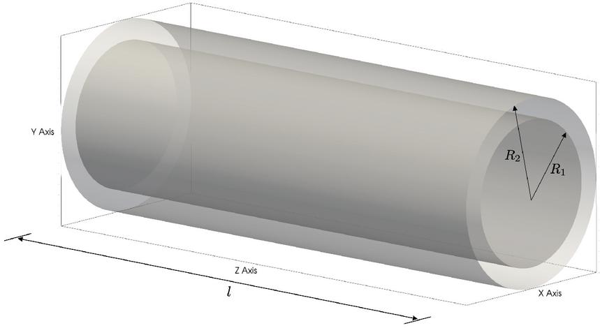
Figure 1 General setup of fluid flow in a cylindrical gap.
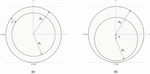
The following Figure 2 shows the corresponding cylinder cross sections in the -plane both without and with eccentricity. The latter case is included here since it is conceptually the most challenging and interesting one; it is also very common in practice as perfect concentricity is rarely obtained in realistic applications.
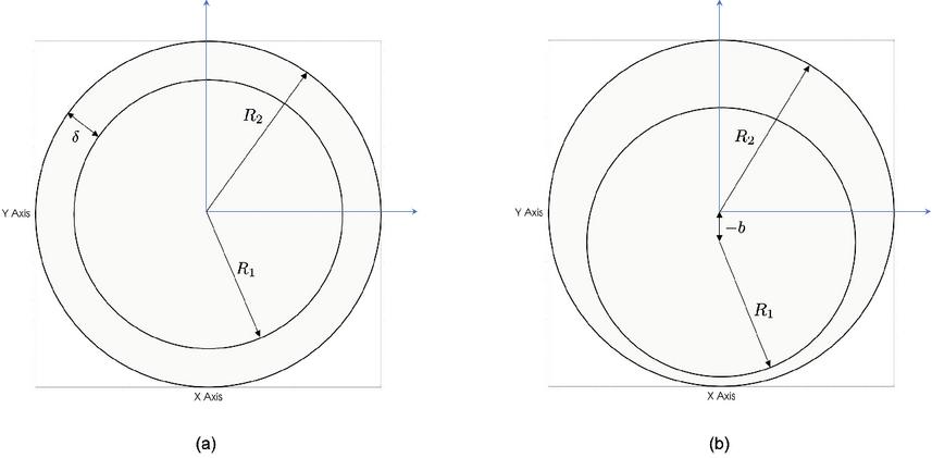
Figure 2 Cross sections of the cylinders of Figure 1, concentric case (a) and eccentric case (b).
In the eccentric case, Figure 2(b), the inner cylinder is displaced vertically from the common symmetry axis by a value of , where is called the absolute eccentricity. On the other hand, the relative eccentricity is defined by , where is the difference between outer and inner radius (see Figure 2(a)).
In this work we will establish a connection between the shear force , that is induced by the viscous flow in between two eccentric cylinders, and its corresponding concentric counterpart by a relation of the form
| (1) |
where is a scale-invariant correction term that only depends on the intrinsic geometry of the system, i.e. the ratio of inner to outer radius, . In particular, is the leading term in a 2nd-order Taylor-expansion of around . As far as we can tell, this relation was unknown previously.
Simplifying even further, since the correction term is a rather complicated expression in , using its derivative to obtain a linear approximation around leads to a very convenient recipe for jet forces in many applications where , i.e.
| (2) |
Following this derivation, we will demonstrate an application of relation (1) in the context of assembling look-up tables for jet forces, which can be used to create a digital twin of hydraulic valves. The concept of a digital twin in this article consists of a complex system-simulation model which includes data from all relevant sub-systems (e.g. fluid forces, magnetic forces, stresses, …). This component is then utilized as a digital twin of hydraulic valves in an automotive system modelling software like Simcenter Amesim.
When implementing the currently available analytical relations for and , due to singular terms the expression for the eccentric case does not reduce easily to the concentric one for . It has to be evaluated either by a limiting process or one would need to switch between and depending on the actual geometry. A similar and well-known situation occurs for the corresponding flow rates and . However, in this case a relation like Equation (2) is known in the form of (see [21])
| (3) |
This approximation is very popular (see for instance [10] or [26]) and is used as state-of-the-art leakage flow model in modern system simulation tools. The proposed Equation (1) is a universal relation for the shear forces and either this expression or its more manageable limit (2) could be implemented as part of the Simcenter Amesim component “BRF01”.
This article is structured as follows: In the following Section 2 the utilization of relation (1) is motivated within the context of generating input data for a digital twin (as defined above). Furthermore, it is reviewed how the current analytical approximations for , , and can be derived from the incompressible, steady-state Navier-Stokes equations and why the currently available relation for does not easily reduce to .
In Section 3 the motivation for the approach chosen here is briefly demonstrated for an already known case. Afterwards, the main result of this work, relation (1) along with the expression for the coefficient , is derived by a Taylor-expansion around . In addition the domain of validity of (1) is discussed, also with regard to approximation (2).
In Section 4 the general setup for the corresponding 3D-simulations of leakage jet forces with Ansys CFX is described. The analytical relation for the jet force is then compared to its proposed approximation as well as to the numerical value obtained in a post-processing step from CFX. This will show the high accuracy of the analytical approximation if the necessary conditions for its application are met.
Finally, in Section 5 the flow rate-curves of the digital twin described in Section 2 are compared to testing results. The good agreement between system simulation and actual measurements motivates the inclusion of 3D-effects into digital twins for hydraulic components. They can be used for the development of hydraulic products that incorporate these components as sub-models.
2 Hydraulic Valves and Digital Twin Technology
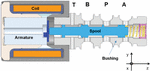
The motivation for deriving relation (1) originates from the necessity to create digital twins for magneto-hydraulic proportional valves as shown in the following Figure 3. The interplay between magnetic and hydraulic forces is harnessed here in order to control the flow of oil to and from the various ports labelled T, B, P and A in the figure below.

Figure 3 Cross section of a typical magneto-hydraulic proportional valve.
There are several different ways, the notion of a digital twin is used in current literature. An approach similar to the one presented here describes a digital twin as a component in a system simulation environment; see e.g. [14]. However, simulation based digital twins may also interact with their hardware surroundings as described in [27]. Additionally they can even continuously evaluate testing data obtained from appropriate sensors; see for instance [12].
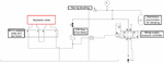
In our case the digital twin is a virtual Amesim representation of the valve depicted in Figure 3 (an Amesim component). The necessary input fields of the magnetic force are computed by axisymmetric 2D-FEM-simulations while the results for the flow forces are based on 3D-FVM-models. The generated data can be incorporated as a parametrized righthand-side for the equation of motion in a system simulation tool such as Amesim. In particular, the relevant CFD-fields which depend on pressure drop, stroke position and fluid temperature can be included in the digital twin by utilizing Amesim’s Signal and Control library. When using this component in a system simulation model of the test rig, the digital twin picks the temperature from the oil property component (labelled “FP04” in the Amesim library) and the corresponding CFD data is used. This general idea is sketched in the following Figure 4.
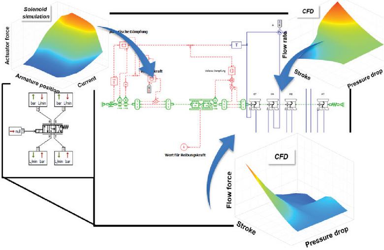
Figure 4 Linking input fields as lookup-tables into a complex, multi-domain system simulation model.
The details of the method described here are not relevant for the main goal of this article; the interested reader is referred to [8] for the magnetic field simulations and to [7, 11] for additional information on the CFD-methods and system simulation. Concerning the flow rate- and jet force-modelling, numerical, analytical and hybrid techniques are available; see for instance [3, 2, 15]. In particular, a contribution modelling flow rates in valves analytically with an orifice equation approach was presented in [23]. There is vibrant activity both in the industrial and academic sector concerning these topics, hence this reference list is not exhaustive at all.
The flow rate and the force that act on the spool of a magneto-hydraulic valve can be computed in a postprocessing step once the velocity distribution is obtained as solution to the incompressible, steady-state Navier-Stokes equation (gravity is neglected here)
| (4) | |||
| (5) |
Equation (4) is the momentum equation for a fluid with density , dynamic viscosity and pressure ; the subsequent Equation (5) ensures conservation of mass in the time-independent and constant-density case considered here.
The PDEs of (4), (5) need to be supplied by proper boundary conditions; in our case these are given by
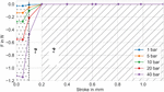
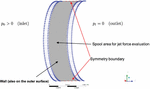
However, when compiling the necessary jet force-fields for the digital twin, the question emerges which values for the forces should be included especially in the overlap area of the stroke. A detailed numerical leakage-simulation of system (4)–(5) for this type of geometry is very time consuming and just setting the fluid force to zero there by brute-force will neglect physical effects and may lead to numerical instabilities; see [18] or [17]. This artificial commitment to vanishing jet-forces when feasible is depicted in Figure 5; numerically computed values are available in a range between 0 mm and 0.1 mm.
The jet forces shown in this figure are negative because the BT fluid flow is directed towards the negative z-direction in the coordinate system of Figure 3 and laminar flows induced by a pressure drop lead to jet forces in direction of the flow (see [4] and the following Equations (7)–(9)).
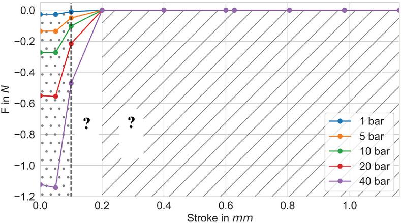
Figure 5 Jet force acting on the spool when the path BT is closed by the spool in Figure 3.
The search for an effective and accurate way of dealing with the regions indicated by question marks in Figure 5 is the main motivation in this article for taking a closer look at analytic relations for the shear force induced by an annular flow between two cylinders.
When the path BT is about to close, the relevant flow domain can be modelled as an annular gap as depicted schematically in Figure 1 and Figure 2. This domain is also depicted in the following Figure 6 for the actual valve used here.
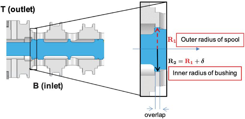
Figure 6 Cross-section view of bushing and spool and zoomed metering edge, where the spool is in a stroke position that closes BT.
Since in this case the flow is dominated by the axial component, the original Navier-Stokes equation reduces to the linear Stokes problem, i.e. an ordinary differential equation; see [21] for example. Using cylindrical coordinates and the divergence constraint (5), the PDE-system (4) can be recast into
| (6) |
with boundary conditions
Here, denotes the axial component of the velocity vector and indicates the pressure drop. The advantage of this type of equation is that for certain flow domains it can be solved analytically. After obtaining the velocity distribution, it is a simple post-processing step to compute the corresponding jet force. The solutions of (6) depend only on the distance to the symmetry axis of the outer cylinder (with Radius ) and integrating them leads straight to flow rates and shear forces. Hence, in cases where the flow is almost purely axial, the Stokes equation already contains the full information of the original system (4)–(5); no time-consuming CFD needed. It is also worth mentioning, that in these cases there is no need for any additional calibration or fitting of the flow rate or flow force as in the case of an analytical orifice equation approach. There, an auxiliary parameter, the so-called discharge or contraction coefficient, is introduced which is not uniquely determined by the Navier-Stokes equations. This coefficient re-implements viscosity-driven effects that are neglected in the Euler- and Bernoulli-equations and are therefore also missing in the resulting orifice equation (see [25] or [13]).
When the relevant shear stresses are integrated over the surface of the inner cylinder, one obtains two different flow force relations, depending on eccentricity. For instance from [4] it is known that in the concentric case, , the jet force acting on the inner cylinder is given by
| (7) |
As described above, this relation is obtained by integrating the corresponding shear stress over the surface of the inner cylinder, i.e.
| (8) |
where the axial velocity component ist given by
| (9) |
Analogously, for the “strict” eccentric case it is known from e.g. [21] that again by integrating the shear stress, the force acting on the surface of the inner cylinder is given by
| (10) |
where
| (11) |
and
| (12) |
An implementable formulation of the corresponding velocity distribution can be found for instance in [22].
Unfortunately as one can see from Equation (10), it is not immediately clear what happens in the concentric case, i.e. for . Simply evaluating this expression for is not allowed since one would divide by . Of course one could compute in a limiting process for ever decreasing values of but this procedure does not at all shed a light on how exactly Equation (10) reduces to Equation (7) in the concentric case.
In the following Section 3 we will therefore derive a practical relation that unites the jet forces for all relative eccentricities, e.g. Equation (1).
3 Analytical Modelling of Leakage Jet Forces
As motivation for our approach, let us start again by considering the different flow rates obtained by solving the Stokes problem for the geometries shown in Figure 2. As already mentioned in the introduction, the flow rate for the eccentric case, , is related to its concentric counterpart by the approximate relation (3), where (see e.g. [21, 26])
| (13) |
Similar to the flow force computation leading to (7), (13) is obtained in a post-processing step by integrating the very same velocity distribution (9), which solves the Stokes Equation (6) within a concentric annulus,
| (14) |
There is also an expression for the corresponding flow rate in the eccentric case, albeit as an infinite series representation (see [21]), given by
| (15) |
Relation (3) seems to be a truncated Taylor-expansion of Equation (15) in the relative eccentricity around , although to the best of our knowledge, the expansion itself is never made explicit in current literature. Now an obvious question related to this discussion is, whether there exists an approximation, relating the jet force of the eccentric case to its concentric counterpart in a similar manner as relation (3) does for the flow rates.
In order to illustrate this point further, let us recall that this approach is already very common in oil hydraulics. The popular approximation (see [10]) for the flow rate in the concentric case
| (16) |
which is also used in the Simcenter Amesim 16.1 component “BAF01” and in DSHPlus (see [20]), is simply the leading term in a Taylor-expansion of Equation (13) around ( is kept fixed there and is replaced by ). In [26] one can even find the next term (of fourth order) in this expansion, which is not widely used in fluid power literature though, i.e.
| (17) |
As a sidenote, it is also rather straightforward to calculate higher-order corrections for this truncated Taylor-series. For example including the fifth order term (not seen by the authors in the literature by now), the corresponding expansion now reads as
| (18) |
Following this idea, Equation (10) for the jet force is regarded as a function of the relative eccentricity and a Taylor-expansion around is carried out. Assuming analyticity of (that is, the Taylor-expansion of (10) is identical to within its convergence radius), we can write
| (19) |
and truncate the expression after the quadratic term. For practical calculations it is actually more convenient to work with the absolute eccentricity as dependent variable since (10) is already expressed in that way. After evaluating the required derivatives, it is an easy application of the ordinary chain rule to switch to as expansion parameter, i.e. .
As a simple example for this approach, let us derive the constant term in (19) which is identical to in (10) and does not include any derivatives at all. The only non-trivial part there is the second term in parentheses; we will consider numerator and denominator separately.
From the Definitions (11), (12) it is clear that
and therefore
| (20) |
For the denominator we write
Now, from (11) we know that for the first two terms in this fraction
and for the third summand
that is (using (20))
Due to continuity of the natural logarithm, putting all this together leads to
| (21) | |||
Since all limits exist, one can then safely divide (20) by (21) and we straightforwardly arrive at
| (22) |
Similar but more tedious calculations involving the first- and second-order derivatives of show that
| (23) |
and finally
| (24) |
Substituting (22)–(24) into Equation (19) and omitting cubic and higher order terms leads to
| (25) |
Replacing in the above expression with Equation (7), factoring out this contribution as well as another term in both numerator and denominator, one finally arrives at relation (1), i.e.
with
| (26) |
This is the main result of this article; a relation that approximates the eccentric shear force by its concentric counterpart and a correction term that depends on the relative eccentricity and the ratio of the radii involved.
While expression (26) is valid for all values of , in many practical applications is close to and therefore . In this case is already specified sufficiently enough by its linear contribution and evaluating the relevant derivative then leads to relation (2), i.e.
This approximation mimics the well-known Piercy-relation for the flow rate and extends it in a similar fashion to jet forces as well.
In order to work out the similarities and differences between the different approaches, we define
| (27) |
and
| (28) |
Both definitions can be understood as expressions mainly dominated by the concentric part but modified by a smaller contribution that depends on eccentricity. This will avoid confusion when we want to compare (15) with its approximation (27) and (10) with (28) respectively.
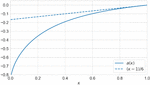
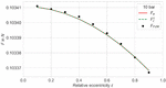
It’s immediately obvious that the constant coefficient of the quadratic correction term in Equation (27) does trivially not include any information about the actual geometry (e.g. the radius of bushing and/or housing in Figure 6). In contrast, the corresponding factor in (28) depends in a rather intricate way on , i.e. the ratio of inner to outer radius; see (26). It is also depicted in the following Figure 7.
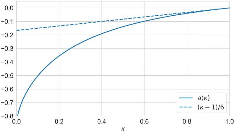
Figure 7 Variation of the correction term and its linear approximation at when increasing the ratio of inner to outer radius.
In addition, the linear approximation of at is shown there as well. As one can see there is a reasonable agreement between these two graphs for .
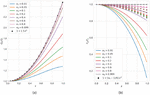
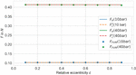
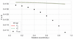
It is worth pointing out, that [21] were well aware of the fact, that their prefactor is not constant at all, but also depends on the ratio of the radii involved. This is depicted in the following Figure 8(a) which compares obtained from (15) on the one hand (solid) with corresponding values computed from (27) on the other hand (dotted); in both cases is evaluated using (13). This figure already appeared in the aforementioned paper and clearly shows that the Piercy-relation (27) is valid only for .
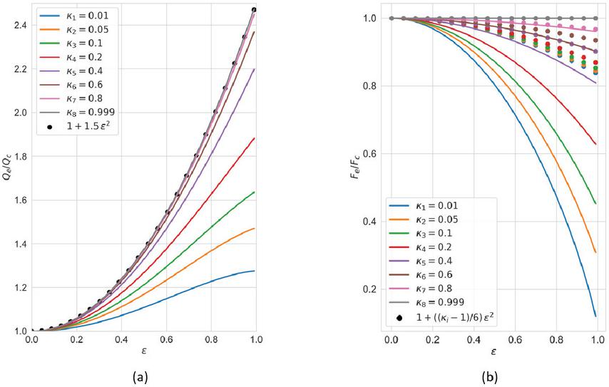
Figure 8 (a) Ratio of eccentric to concentric flow rates and (b) corresponding jet forces (solid), as well as their proposed approximations which are valid for (dotted).
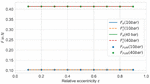
Figure 8(b) shows a similar comparison for the jet forces, i.e. (10) vs. (2); is obtained from (7). One can clearly see that the simple relation (2) is a very good approximation as long as and can therefore be regarded as equivalent to the Piercy-relation for the flow rate.
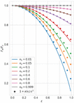
However, in addition to Equation (2) we also derived the entire corresponding 2nd-order approximation (in relative eccentricity ); see relation (28). It should adequately describe the behaviour of the jet forces for an even wider range of possible . This is indeed the case as can be seen in the following Figure 9.

Figure 9 Comparison of relative jet forces, exact (solid) vs. full 2nd-order approximation (dotted).
In contrast to the previous case it is obvious that Equation (28) proposed in this paper is a suitable approximation for all values of . Only when considering large eccentricities and huge differences between inner and outer radius, higher-order corrections to (28) become relevant. But as already mentioned before, in the same regime where the Piercy-relation holds, (28) could easily be replaced by its much simpler version (2).
In order to further check the accuracy of both and its suggested alternative , the following Section 4 will compare them with results obtained from 3D CFD-simulations.
4 Numerical Modelling and Comparison of Leakage Jet Forces
In order to evaluate whether the assumption of a purely axial flow is in fact justified in the cases studied here, a 3D-simulation is performed in the leakage flow domain between bushing and spool as depicted in Figure 6.
The initial overlap in our example valve was 0.6 mm, however different designs might also lead to different overlaps so as a second test case, a value of 1.55 mm was chosen as well. The task is then to solve the laminar and incompressible, steady-state Navier-Stokes system (4),(5) for prescribed geometries and boundary conditions.
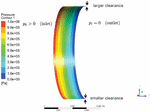
Ansys CFX was used to carry out FVM-simulations for the general setup described in Section 1 and depicted in Figures 1, 2. The following Figure 10 illustrates in more detail the computational domain and the boundary conditions chosen here.
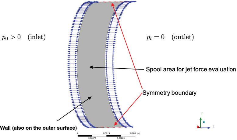
Figure 10 Half symmetric computational domain and corresponding boundary conditions for 1.55 mm overlap; only the inner cylinder surface is visible.
Some relevant information about the geometrical and numerical specifications for the simulations is summarized in Table 1.
Table 1 Summary of parameters for numerical leakage simulation
| Data | Value | Unit |
| 10 & 40 | bar | |
| 3.29 | mm | |
| 3.3 | mm | |
| 0.997 | – | |
| 10.11 | mPa s | |
| 805 | kg/m | |
| mm | ||
| 0.6 & 1.55 | mm | |
| no. of nodes (overlap 0.6 mm) | 1,012,112 | – |
| no. of elements (overlap 0.6 mm) | 932,400 | – |
| no. of nodes (overlap 1.55 mm) | 2,588,352 | – |
| no. of elements (overlap 1.55 mm) | 2,408,700 | – |
Particular care has to be taken of an appropriate meshing of the computational domain. For cases in which the flow is dominated mainly by the axial velocity component and varies smoothly with distance from the symmetry axis, a sweep meshing method with radial boundary refinement is used; see the following Figure 11 as an example.
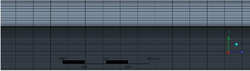
Figure 11 Mesh for the expected laminar fluid flow, dominated by the axial component.
In order to compare the analytical expression for , i.e. relation (10), and its proposed approximation (which by contrast trivially includes the concentric case, see Equation (28)) to numerical results, the jet force obtained from the 3D-simulations is evaluated for eccentricities .
In the following Figure 12 one can see, how well our relation for the jet force performs when benchmarked against both numerically obtained forces and the original analytical relation for .
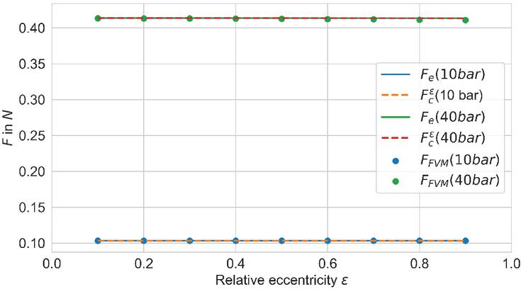
Figure 12 Comparison of numerically and analytically obtained jet forces for 10 bar and 40 bar pressure drops and an overlap of 0.6 mm.
For the comparison shown in Figure 12, an overlap of 0.6 mm was used. However, results are identical for the second test case considered here, i.e. an overlap of 1.55 mm; see the following Figure 13. As expected from the analytic expressions, there is no noticeable influence of the overlap on the jet forces; they are virtually identical for both values considered here.
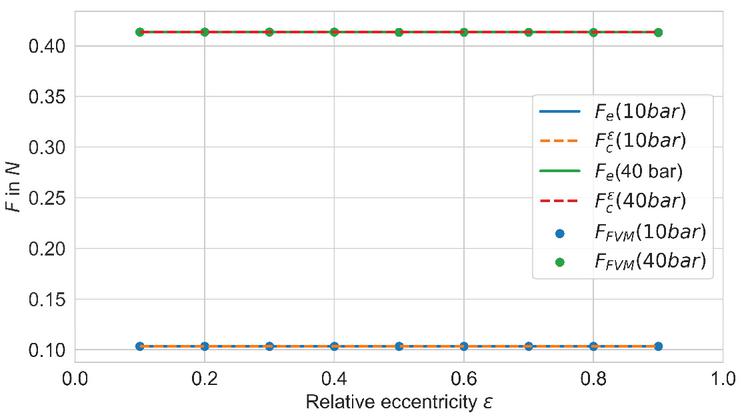
Figure 13 Comparison of numerically and analytically obtained jet forces for 10 bar and 40 bar pressure drops and an overlap of 1.55 mm.
The relative difference between the proposed relation (28) and the numerical results is less than 0.6 % which emphasizes the good accuracy of our approximation for . The reason for this agreement is partly because the requirements for its application are met in this case, i.e. a clearly laminar behaviour of the fluid flow as highlighted in the following Figure 14 (see also Figure 10).

Figure 14 Linear pressure distribution for an overlap of 1.55 mm, relative eccentricity of 0.8 and a 10 bar pressure-drop.
Even though it is not apparent from Figures 12, 13, the quality of the approximation proposed in this article depends on the correctness of its underlying assumptions, one of them being that the resulting flow can be described by the linear Stokes equation, therefore neglecting turbulence. The following Table 2 summarizes Reynolds number (Re) and maximum values of the velocity components in the Cartesian system used for the simulation. Keep in mind, that in the nomenclature developed in Sections 2 and 3.
Table 2 Reynolds number and component-wise speed maxima obtained from the CFD-simulations, velocities are given in .
| 10 bar, 0.6 mm | 10 bar, 1.55 mm | 40 bar, 0.6 mm | 40 bar, 1.55 mm | |
| Re | 66.61 | 35.53 | 262.02 | 141.77 |
| 0.18 | 0.04 | 0.96 | 0.32 | |
| 0.40 | 0.1 | 1.91 | 0.71 | |
| 6.59 | 2.55 | 25.7 | 10.3 |
It’s obvious from the data presented in Table 2, that the simulation with a pressure difference of 10 bar and an overlap of 1.55 mm leads to the smallest Reynolds number as well as the largest ratio of axial to radial velocity components, that is . This would signal both a laminar and an axially dominated flow, i.e. the two assumptions that are prerequisites for applying the proposed relation (28). On the other hand, based on the same reasoning one would expect the largest deviation from our approximation in the corresponding simulation of a 40 bar-pressure drop and an overlap of 0.6 mm.
These predictions are corroborated by the following Figures 15 and 16, which are zoomed-in versions of the relevant curves already depicted in Figures 12, 13.
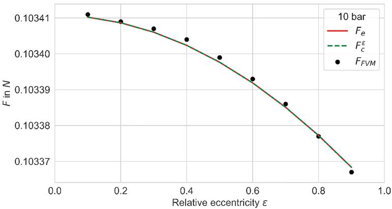
Figure 15 Comparison of numerical and analytical forces for a 10 bar pressure drop and an overlap of 1.55 mm (scaled-up from Figure 13).
Although the differences are minuscule from a practical point of view, the figures still show vividly how good relation (28) approximates the analytical solution (10) of the linear Stokes equation and how both approaches, strictly speaking, fail once the corresponding fluid flow gets more turbulent and less axially dominated.
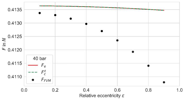
Figure 16 Comparison of numerical and analytical forces for a 40 bar pressure drop and an overlap of 0.6 mm (scaled-up from Figure 12).
On the other hand, especially Figures 12 and 13 show that apart from this rather academic discussion, even stronger violations of the assumptions required for applying (28) still lead to a good estimate of the jet forces for all practical purposes. A rigorous study of the sensitivity of the proposed approximation with respect to the ratio (annular gap divided by overlap) with methods from asymptotic analysis (as used in [19]) could be the content of future work.
The following Figure 17 finally answers the question of how the jet forces can be modelled when the path BT is closed. For geometries like concentric or eccentric gaps, analytical approximations like relation (28) are applicable.
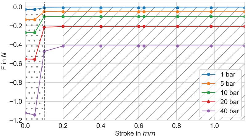
Figure 17 Completion of numerically obtained shear forces by analytically computed shear forces; compare with Figure 5.
The last Section 5 will describe an experimental setup to gauge the accuracy of the combined numerical/analytical model of the jet forces for usage in a digital twin.
5 Experimental Testing and Validation of the Combined Model
In order to illustrate the accuracy of the response from the digital twin schematically depicted in Figure 4, numerical and analytical input fields were generated by post-processing 3D-simulations as well as utilizing relations like (27) and (28). The digital twin described in Section 2 is then included in an Amesim model of the hardware test rig. The oil temperature (determined by the ambient temperature of the climate chamber), which dictates the relevant CFD-fields for the system simulation model, can be set via the Amesim component ”FP04”; see also [7] or [11] for further details on using input data with Amesim. Finally, the numerically obtained flow rates are compared to corresponding measurements from the test rig, including the hardware twin of the valve.
The following Figure 18 depicts the Hilite test rig used for hydraulic measurements of a flow regulating valve. Since the test bench is employed for other measurements as well, the overall setup shown here is slightly larger than required.

Figure 18 Test rig used for measuring flow rates; the red arrow points to the actual valve within this setup.
The reduced hydraulic scheme corresponding to this setup is depicted in Figure 19; the actual valve that is marked by an arrow in previous Figure 18 is outlined in red here.
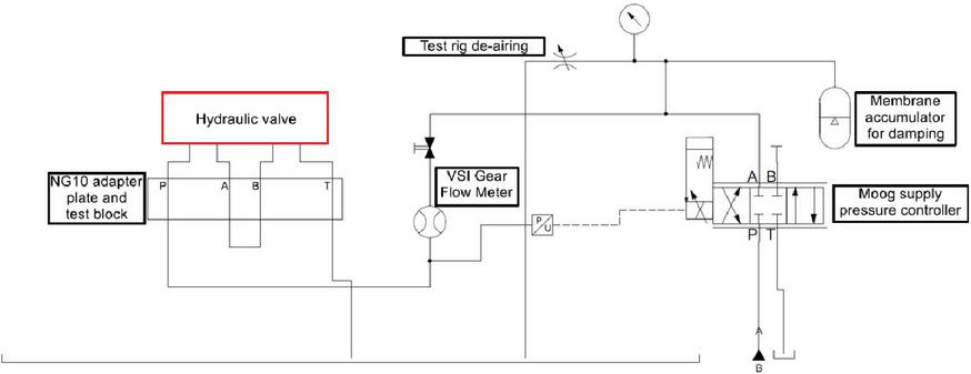
Figure 19 Reduced hydraulic scheme; the valve to be measured is outlined in red.
A direct acting servo valve by Moog is used for adjusting the supply pressure. It features a very short response time and is used in our test benches for facilitating static supply pressures and to eliminate pressure differences during each single test. The built-in accumulator prevents undesired pressure oscillations. Prior to the inlet a VSI gear flow meter is employed for measuring the flow rate. In this type of device gear rotation is monitored by a non-contacting signal pickup system. This allows for a precise determination of the fluid volume that is enclosed in the measuring chambers between the gear teeth. The VSI is a pre-amplifier that greatly improves signal quality, leading to measurement errors below 0.3% within a temperature range from 40 C to 120C.
A Kulite pressure sensor placed between gear flow meter and valve is used in a feedback-loop with the Moog controller to monitor and adjust the pressure on the inlet of the valve. The sensor is calibrated for all specified temperatures before starting any flow measurements in order to achieve a high accuracy.
For measurements at different temperatures the entire test rig can be put into a CTS conditioning chamber; see the following Figure 20.
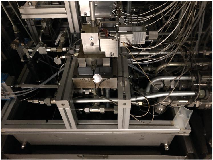
Figure 20 Interior view of the CTS temperature test chamber.
In this way, it is possible to simulate and adjust for environmental influences on the valve as well as attached transmission components. This is a standard test procedure for automotive testing and it allows for separate heating/cooling of fluid and environment. The CTS chamber is set to the required temperature and in addition, the fluid (oil in this case) is also cooled or heated. When the chamber has reached the necessary temperature there is an auxiliary holding time of about 6 hours so that chamber, fluid and test rig can achieve thermal equilibrium.
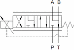
A schematic diagram of the measured valve is depicted in the following Figure 21.
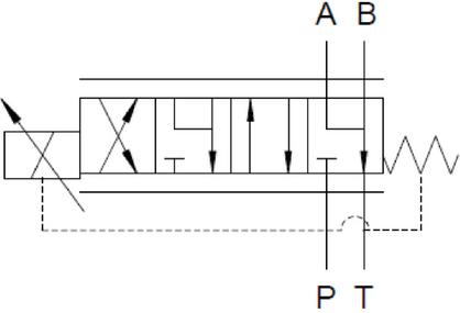
Figure 21 Fluid circuit diagram of the valve used for testing.
In this case, it is a 4/4 proportional valve with an adjustable solenoid acting from the left (as indicated by the corresponding symbol, see also Figure 3). In its neutral position, a floating condition is achieved while blocking the connection to the pump and no fluid flow will occur. Once energized, the solenoid will move the spool inside the bushing so that with increasing stroke fluid is passing from pressure inlet P (a supply pressure of 10 bar is applied here) to port A and from port B back to the reservoir T respectively. Moving further, another floating position with zero volume flow is reached before the high pressure inlet P is connected to B and accordingly port A back to the reservoir T.
For measurements the solenoid contained within the valve is subjected to a current ramp. After a brief currentless activation at the start of this routine (automated postprocessing of data is initiated here), the electric current is increased with a ramp speed of 33 mA/s before reaching its final value of 1000 mA after roughly 30 seconds. From this maximum the current is decreased to 0 A at the same speed. In addition to this current ramp there is also a harmonic dither-signal with a frequency of 125 Hz and an amplitude of 250 mA which is superimposed to the carrier current.
The following Figure 22 depicts the time-dependent current variation outlined above.
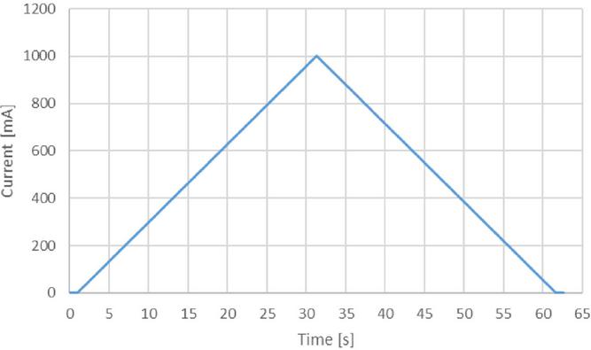
Figure 22 The variation of electric current with time used for the flow rate measurements; dither-signal not included here.
All signals are recorded with an initial sampling frequency of 30 kHz and are then subsequently downsampled to 10 kHz in order to reduce the amount of data to be processed. As required by most of the customers, the signals are filtered afterwards with a 4th-order Bessel filter employing a cutoff-frequency of 10 Hz and separated into rising and falling segments according to the current ramp of Figure 22.
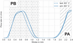
The following Figure 23 shows the characteristic flow curve obtained as an average over rising and falling segments for the digital twin and compares it to the corresponding measurements at an operating temperature of 60 C. Due to required confidentiality, the -axis needs to remain unlabelled.
Figure 23 Comparison between simulated and measured flow rate (average of rising and falling segments) at a temperature of 60 C.
As one can see, the agreement between simulation and measurement is very good. The areas in which PA and PB are open are marked with point and line patches respectively. The flow outside of the marked areas is due to partial openings due to the spool geometry (see Figure 3), the connection of PB and AT and PA and BT respectively and internal leakage. This also extends to other temperatures as well; see the following Figure 24.
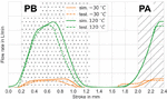
Figure 24 Same as Figure 23 but for 30 C and 120 C.
As expected, mainly due to viscous effects which increase for lower temperatures, the flow rates decrease significantly when dropping the temperature; see also Equations (13), (15). While there are slightly larger deviations between simulation and measurement, the overall agreement is still satisfactory.
This comparison shows the usefulness of employing proper modelled digital twins of valves in system simulations in order to optimize the performance of these elements as components of larger transmission assemblies.
6 Conclusion
In this work an analytical approximation for the shear force, which is induced by viscous flow between two cylinders, is presented. This relation, as well as its derivation, mimics the well-known Piercy-approach for the corresponding volume flow which involves the relative eccentricity as an expansion parameter for a Taylor-series. While the latter one is strictly valid only in a certain limiting case (that is nevertheless mostly fulfilled in practical applications), the approximation for the shear forces proposed here exhibits a much broader range of validity. Its utilization is restricted only by the inherent limitation of a truncated series expansion and the requirement of a laminar, axially dominated fluid flow.
These findings were corroborated by comparisons with 3D-simulations of the complete Navier-Stokes equations. The detailed case studies not only showed under which circumstances our approximation will fail to hold but also how minute the observed discrepancies between analytical and numerical results are. From this point of view, our statement about the suggested domain of validity is rather a mathematical conclusion than something that would severly limit the application of our relation for the jet forces in any realistic scenario. In fact, it could be implemented quite universally for example in subsequent releases of the Simcenter Amesim component “BRF01”. This would also neatly fit with other components, e.g. “HYDORG11”, that already utilize similar analytical estimates.
As an application example, the proposed approximation for jet forces was applied for the generation of input fields for a digital twin. These are needed by system simulation software in order to accurately predict the behaviour of actual, real devices on which the corresponding digital counterparts are based upon. Proper modelled components also help to optimize preliminary designs in a cost-effective manner. Of course, the success of this approach stands and falls by the accuracy of the digital reproduction of a physical object. The procedure presented here in case of a magneto-hydraulic valve leads to a very good agreement between simulation and measurements. This will undoubtedly encourage and foster the development of hydraulic systems by exchanging digital twins between vendors and customers in a modern, networked environment.
7 Nomenclature
| R1 | radius of inner cylinder |
| R2 | radius of outer cylinder |
| δ | annular gap/clearance between cylinders, i.e. |
| κ | ratio of inner and outer cylinder radius, i.e. |
| b | absolute eccentricity/shift of inner cylinder |
| ε | relative eccentricity/shift of inner cylinder, i.e. |
| p0 | pressure at inlet |
| pl | pressure at outlet |
| Δp | pressure drop, i.e. |
| Fe | flow force in the eccentric case |
| Fc | flow force in the concentric case |
| Qe | flow rate in the eccentric case |
| Qc | flow rate in the concentric case |
| Qcε | known approximation of eccentric flow rate, as correction of |
| Fcε | new approximation of eccentric jet force, a truncated expansion of |
| Q1 | leading term of Taylor-expansion of in , around |
| Q2 | first two non zero terms of mentioned Taylor-expansion of |
| Q3 | first three terms of mentioned Taylor-expansion of , not seen by authors in literature |
| μ | dynamic viscosity of fluid |
| ρ | density of fluid |
| v | fluid velocity field, whith radial components , and axial contribution |
| p | pressure of fluid |
References
[1] Yutaka Abe, Hajime Akimoto, and Yoshio Murao. Estimation of shear stress in counter-current annular flow. Journal of Nuclear Science and Technology, 28, 1991.
[2] Riccardo Amirante, Elia Distaso, and Paolo Tamburrano. Sliding spool design for reducing the actuation forces in direct operated proportional directional valves: Experimental validation. Energy Conversion and Management, 119, 2016.
[3] Riccardo Amirante, G. Vescovo, and Antonio Lippolis. Flow forces analysis of an open center hydraulic directional control valve sliding spool. Energy Conversion and Management, 47, 01 2006.
[4] R.B. Bird, E.N. Lightfoot, and W.E. Stewart. Transport Phenomena. J. Wiley, 2002.
[5] Patrik Bordovsky, Katharina Schmitz, and Hubertus Murrenhoff. Cfd simulation and measurement of flow forces acting on a spool valve. In 10th International Fluid Power Conference , Dresden , Germany, 2016.
[6] Wilson C. Chin. Chapter 4 - steady, two-dimensional, non-newtonian, single-phase, eccentric annular flow. In Wilson C. Chin, editor, Managed Pressure Drilling. Gulf Professional Publishing, 2012.
[7] Christian Hugel. Optimization of a piston geometry in a pressure control valve. RDO Journal Issue 2, 2016.
[8] Christian Hugel. Optimization of an actuators magnetic force with optislang. RDO Journal Issue 2, 2019.
[9] D. Joseph, Ruijing Bai, Kang Chen, and Yuriko Renardy. Core-annular flows. Annu. Rev. Fluid Mech., 29, 11 2003.
[10] E.M. Khaĭmovich. Hydraulic Control of Machine Tools. Pergamon Press, 1965.
[11] Johannes Krebs. optislang in functional development of hydraulic valves. RDO Journal Issue 2, 2019.
[12] Francois Laborie, Ole Christian Røed, Geir Engdahl, and Audrey Camp. Extracting value from data using an industrial data platform to provide a foundational digital twin. Offshore Technology Conference, 2019.
[13] L.D. Landau and E.M. Lifshitz. Fluid Mechanics: Volume 6. Elsevier Science, 2013.
[14] Ryan Magargle, Lee Johnson, Padmesh Mandloi, Peyman Davoudabadi, Omkar Kesarkar, Sivasubramani Krishnaswamy, John Batteh, and Anand Pitchaikani. A simulation-based digital twin for model-driven health monitoring and predictive maintenance of an automotive braking system. 2017.
[15] Noah Manring. Modeling spool-valve flow forces. ASME 2004 International Mechanical Engineering Congress and Exposition, 2004.
[16] Mario Neto and Luiz Goes. Use of lms amesim model to predict behavior impacts of typical failures in an aircraft hydraulic brake system. In Proceedings of 15th Scandinavian International Conference on Fluid Power, pages 29–43, 12 2017.
[17] Jarmo Nurmi and Jouni Mattila. Detection and isolation of leakage and valve faults in hydraulic systems in varying loading conditions, part 1: Global sensitivity analysis. International Journal of Fluid Power, 2011.
[18] Michael Païdoussis. Annular- and Leakage-Flow-Induced Instabilities. 12 2016.
[19] Grigory Panasenko and Konstantin Pileckas. Asymptotic analysis of the nonsteady viscous flow with a given flow rate in a thin pipe. Applicable Analysis, 91, 2012.
[20] Enrico G. Pasquini. Eindimensionale Berechnung instationärer Ringspaltströmungen mit thermofluiddynamischer Betrachtung. Reihe Fluidtechnik, RWTH Aachen, 2020.
[21] N.A.V. Piercy, M.S. Hooper, and H.F. Winny. Liii. viscous flow through pipes with cores. The London, Edinburgh, and Dublin Philosophical Magazine and Journal of Science, 1933.
[22] R.K. Shah and A.L. London. Laminar flow forced convection in ducts. Academic Press, 1978.
[23] Marko Šimic, Mihael Debevec, and Niko Herakovič. Modelling of hydraulic spool-valves with special designed metering edges. Strojniški vestnik-Journal of Mechanical Engineering, 60(2):77–83, 2014.
[24] Jeffrey Tithof, Douglas H Kelley, Humberto Mestre, Maiken Nedergaard, and John H Thomas. Hydraulic resistance of periarterial spaces in the brain. Fluids and Barriers of the CNS, 16, 2019.
[25] Frank M White. Fluid mechanics. Tata McGraw-Hill Education, 1979.
[26] Frank M. White. Viscous fluid flow. McGraw-Hill New York, 2006.
[27] Holger Zipper, Felix Auris, Anton Strahilov, and Manuel Paul. Keeping the digital twin up-to-date — process monitoring to identify changes in a plant. 2018 IEEE International Conference on Industrial Technology (ICIT), 2018.
Biographies

Zoufiné Lauer-Baré currently works as simulation engineer in the development of electro-hydraulic valves. He received his Ph.D. in 2014 at the Fraunhofer Institute for Industrial Mathematics (ITWM) and the TU Kaiserslautern. The topic of his thesis was the modeling of elastic rod structures.

Erich Gaertig finished his Ph.D. in theoretical astrophysics at the University of Tübingen in 2008. After further postdoc studies and a short interlude as development engineer, working on novel numerical approaches, he joined the simulation group at Hilite. There, he is mainly responsible for electromagnetic field calculation of actuators. Other areas of interest include modelling and numerical/analytical methods in physics and engineering.

Johannes Krebs currently works as a simulation manager at the simulation department. He is responsible for the transmission simulation. After he finished his thesis in numerical fluid- and aerodynamics at the University of Stuttgart (IAG) in 2014, he started at Hilite as a CFD-simulation specialist. Other fields he is working on are system simulation and the modelling of digital valve systems including DOE and robust design analysis.

Christian Arndt finished his study of Aerospace Engineering at the University of Stuttgart in 2008. After that he worked as simulation engineer in the development of gasoline engines with focus on 1D- and 3D-CFD simulations. He joined Hilite in 2016 where his field of work are system simulations as well as 3D-CFD simulations in the development of hydraulic cam phaser systems.

Christian Sleziona received his Ph.D. in Plasma Propulsion at the University of Stuttgart. He finished his postdoctoral thesis on Hypersonic Flows and started as professor for Hypersonic Aerothermodynamics at Tohoku University in Japan. After working at the ITWM of the University of Kaiserslautern and IHI Charging Systems International, he currently works as head of the simulation department at Hilite.

André Gensel currently works as a manager at testing department. He is responsible for transmission valve testing. He joined Hilite in 2014 after he finished his diploma thesis in reducing of drag torque on wet running multi-plate clutch systems at Brandenburg University of Technology (BTU).
International Journal of Fluid Power, Vol. 21_1, 113–146.
doi: 10.13052/ijfp1439-9776.2214
© 2021 River Publishers