Model-based Simulation of a Hydraulic Closed-loop Rotary Transmission with Automatic Control

Gunnar Grossschmidt^1,* and Mait Harf²

¹Department of Mechanical and Industrial Engineering, Tallinn University of Technology, Tallinn, Estonia

²Department of Software Science, Tallinn University of Technology, Tallinn, Estonia

E-mail: gunnar.grossschmidt@ttu.ee; mait@cs.ioc.ee

^*Corresponding Author

Received 12 October 2020; Accepted 06 December 2020; Publication 27 April 2021

Abstract

Model-based simulation of a hydraulic closed-loop rotary transmission with automatic control of hydraulic pump and hydraulic motor is considered in the paper. The approach is based on multi-pole modelling and intelligent simulation. In the paper the functional scheme of the transmission is proposed and multi-pole models of components are introduced. Mathematical multi-pole models of components for steady state conditions and for dynamic transient responses are presented. A high-level graphical environment CoCoVila (Compiler Compiler for Visual Languages) is used as a tool for describing models and performing simulations. Object-oriented multi-pole models, visual programming environment, automatic program synthesis and distributed computing are as original approach in simulation of fluid power systems.

Keywords: Hydraulic closed-loop rotary transmission, automatic control, multi-pole mathematical model, intelligent simulation environment, visual task description, automatic program synthesis.

1 Introduction

Power transmission is the movement of energy from its place of generation to a location where it is applied to perform useful work. In a hydrostatic rotary transmission hydraulic energy is generated in a hydraulic pump. The energy is used in a hydraulic motor to perform useful work. There are two main types of hydraulic rotary transmission compositions – open- and closed-loop transmissions. Closed-loop transmission requires less tank thus it is preferable in mobile machines. An electric or a combustion engine can be used to drive a hydraulic pump. The latter is preferred in transmissions of mobile machines. In the paper we consider a rotary transmission for low power mobile machines mainly as it is more compact in size and infinitely variable despite the fact that efficiency coefficient of a hydraulic transmission is lower than mechanical transmissions. Rotary transmissions of simple configuration containing only a pump and a hydraulic motor are observed (Murrenhoff 2005, Parambath 2016, Zhang 2019). Mainly output angular speed, moment, power and efficiency coefficient are calculated. The catalogues describe adjustable hydraulically and electrically controlled pumps and motors that maintain a constant drive speed, constant torque and constant power (Bosch Rexroth AG 2005). A hydraulic servo-system with feedback that controls the position of the swash plate of the pump or the hydraulic motor is described in (Bosch Rexroth AG 2005, Park et al. 2002).

A hydro-mechanical transmission is used in small tractors, where the hydraulic transmission is connected to a mechanical planetary gearbox which allows part of the power to be transferred mechanically (Cao and Zhang 2010, Seok Hwan Choi et al. 2013). STEYR presented its first tractors with continuously variable transmissions in 1999 (Aitzetmüller 2000). The engine and transmission are regulated automatically by the S-tronic system depending on load, and easily controlled with the Multicontroller or accelerator pedal (parallel mode). In 2000, STEYR launched the first tractors with continuously variable transmissions in the power range 120 to 170 hp. This technology is today still the benchmark in the higher power classes.

Designing automatically controlled hydraulic systems in experimental way is time consuming and expensive. One of the first steps in designing such a multi-component transmission is to model and simulate it on a computer, which allows better solutions and more efficient parameters to be found. Modelling and simulation of rotary transmission have been discussed in several published works (Vacca et al. 2007, Cao and Zhang 2010). The hydro-mechanical transmission (HMT) tractor simulator (Seok Hwan Choi et al. 2013) consists of the AMESim model of the HMT, engine and tractor dynamics and MATLAB/Simulink interface of the driver model, a controller, and a road load.

In the paper model-based intelligent simulation of a complex hydraulic closed-loop rotary transmission system with an automatic adjustment range is considered. Hydraulic closed-loop rotary transmission under consideration consists of a variable displacement pump driven by a diesel engine, a variable displacement hydraulic motor, regulators for angle inclination of swash plates, a feeding pressure relief valve and a flushing pressure relief valve, the hydraulic hoses, valves and auxiliary equipment. The hydraulic pump and the hydraulic motor are automatically controlled depending on load moment to the transmission. Modelling and simulation of steady state conditions and dynamic responses of the hydraulic transmission are considered.

Multi-pole mathematical and graphical models (Grossschmidt and Harf 2009a, 2010, 2012, 2016, 2018; Harf and Grossschmidt 2013, 2014, 2015) are used to describe the rotary transmission. Visual programming environment CoCoViLa (Grigorenko et al. 2005, Grigorenko and Tyugu 2006, Kotkas et al. 2011) is used as a tool for graphical modelling and simulation. CoCoViLa supports declarative programming in a high-level language and automatic program synthesis. Using multi-pole models of components enables to use distributed simulation of steady state conditions and dynamic transient responses. In this way we can avoid compiling and solving large differential equation systems.

Automatic control system proposed in the paper does not contain sensors, proportional valves, servo-valves and electronic equipment. Therefore it is of a quite simple configuration and is expected to be more reliable and cheaper.

2 Functional Scheme of a Closed-loop Hydraulic Rotary Transmission with Automatic Control

The functional scheme of a closed-loop hydraulic rotary transmission with automatically controlled hydraulic pump and hydraulic motor is shown in Figure 1.

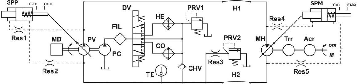
Figure 1 Functional scheme of a closed-loop hydraulic rotary transmission with automatic control.

In Figure 1 components of transmission are denoted as follows:

Acr – rotation actuator

CHV – check valve

CO – cooler

DV – directional valve

FIL – filter

H1, H2 – hydraulic hoses

HE – heater

MD – diesel engine

MH – automatically controlled variable displacement hydraulic motor

PC – fixed displacement feeding hydraulic pump

PRV1 – feeding pressure relief valve

PRV2 – flushing pressure relief valve

PV – automatically controlled variable displacement hydraulic pump

Res1…Res5  – hydraulic resistors

SPM – hydraulic motor swash plate with control piston

SPP – hydraulic pump swash plate with control piston

TE – contact-thermometer

Trr – speed reducer.

To ensure wide control range, simultaneous control of hydraulic pump and hydraulic motor takes place in dependence of load moment. Pressure differences at pump and motor outlet and inlet are used to characterize the load moment. Increasing load moment the swash plate position angle of the pump (pump working volume) decreases and swash plate angle of the motor (motor working volume) increases. At the same time angular speed of the working mechanism decreases. Maximum load moment is limited by maximum moment developed by the diesel engine, maximum moment of the hydraulic motor and the safety valve (not shown in the scheme). The speed reducer Trr is used for adjusting the drive to requirements of the rotation actuator Acr. To compensate volumetric losses (in both, pump and motor) and flushing flow a feeding pump PC is included. Feeding pump flow passes filter FIL and the directional valve DV that directs the flow through the heater HE or the cooler CO. Switching takes place according the signal from contact-thermometer TE. Part of the feeding pump flow is directed back to the tank through the pressure relief valve. Feeding pressure relief valve PRV1 guarantees constant pressure feeding of the main pump suction side. Flushing pressure relief valve PRV2 guarantees constant pressure flushing. Pressure relief valves are considered to consist of three components: poppet valve, flow opening of poppet valve and spring retainer. Check valve CHV avoids possible feeding flow in opposite direction at some moment of the dynamic transient response. In flushing chain part of the feeding flow is directed back to the tank through the connected in series hydraulic resistor (determines the flushing flow) and flushing pressure relief valve PRV2. As a result part of working fluid is continuously excluded from the circulation and is replaced with fresh fluid (flushing).

3 Multi-pole Model of the Transmission

Multi-pole mathematical models are used that adequately describe the physical processes in hydraulic and mechanical systems. The direct actions and feedbacks are expressed in component models.

Each component of the system is represented as a multi-pole model having its own structure including outer variables (poles), inner variables and relations between variables. Multi-pole models of components can be connected together only using poles. Poles can represent input or output variables of the component according the causality of the model.

The causalities of multi-pole models of components will be selected depending on:

• process of simulation (steady state conditions, dynamic transient response)

• the physical causality

• the obligatory causalities of separate devices

• possible variants of connecting the multi-pole models

• to avoid the “mathematical stiff” dependencies.

A component model can enclose nonlinear equations, inner iterations, logic functions and calculation programs as relations. Multi-pole model of the whole system doesn’t need substantial simplification. So we can perform simulations, taking into account adequately the dependencies of all components.

Using multi-pole models enables methodical, graphical representation of mathematical models of large and complicated systems. In this way we can be convinced of the correct composition of models and we don’t need to check the solvability. It is possible directly simulate the steady state conditions without using differential equation systems.

Implementing multi-pole models for each component gives us possibility to compose graphically the simulation tasks and to use distributed simulations. Calculations are performed in each model separately. This simplifies the simulation. To solve loop dependences between component models the iteration method is used.

Model of steady state conditions of the hydraulic rotary transmission with automatic control is shown in Figure 3. Model of dynamics of the transmission is similar except models of pressure relief valves having different inputs and outputs.

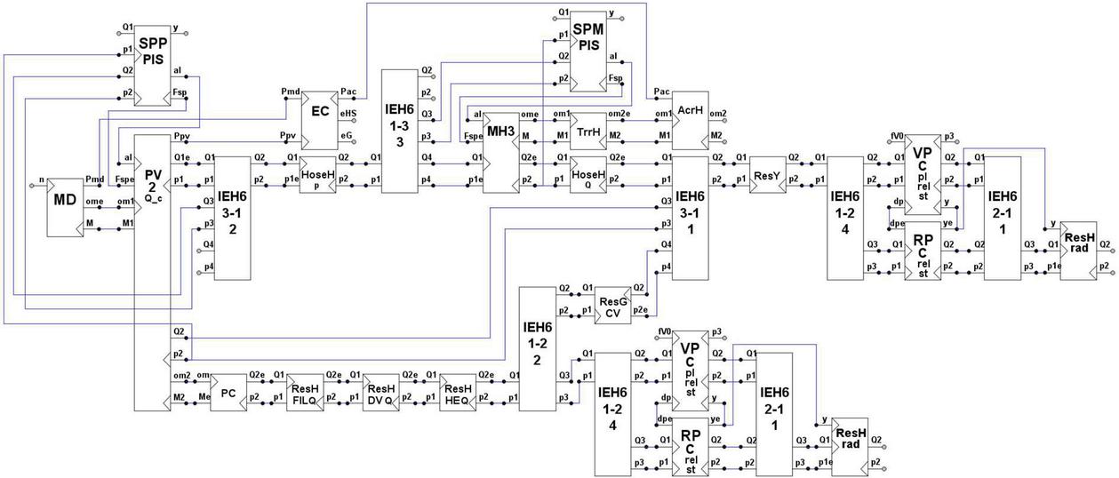
Figure 2 Multi-pole model of steady state conditions of the closed-loop hydraulic rotary transmission with automatic control.

In Figure 2 the following multi-pole models of transmission components are shown:

AcrH – rotary actuator

EC – efficiency coefficient calculator

HoseH_Q, HoseH_p – hydraulic hoses

IEH – hydraulic interface elements

MD – diesel engine

MH3 – hydraulic motor

PC – hydraulic feeding pump

PV2_Q – hydraulic pump

ResH_DV – direction valve as resistor

ResH_FIL – filter as resistor

ResH_HE – heater as resistor

ResH_rad – pressure relief valve spring retainer as resistor

ResY, ResG – hydraulic resistor

RPC_rel_st – feeding and flushing pressure relief valve opening to flow of steady state conditions

SPM_PIS – hydraulic motor swash plate with regulating piston

SPP_PIS – hydraulic pump swash plate with regulating piston

TrrH – speed reducer

VPC_pl_rel_st – feeding and flushing pressure relief valve poppet of steady state conditions.

The model for dynamics of the rotary transmission contains a set of resistors ResG to dampen vibrations. Also, the models of hydraulic pressure relief valves for dynamics are different.

VPC_pl_rel_dyn – feeding and flushing pressure relief valve poppet of dynamics

RPC_rel_dyn – feeding pressure relief valve opening to flow of dynamics

RPPC – flushing pressure relief valve opening to flow of dynamics.

4 Mathematical Multi-pole Models of Components

Mathematical multi-pole model of a component contains variables and formulae that express dependencies between variables. Some of variables are defined as input or output variables, latter are used for interaction with other components.

In general mathematical models of components for steady state conditions and dynamic transient responses are different. +In the models where the role of dynamics is minimal, formulae of steady state conditions are used for dynamics as well.

When describing mathematical models of components for dynamics, mathematical relations are expressed through differences. The fourth-order classical Runge-Kutta method is used for integration in component models.

The values of parameters of components used in the simulations must be specified. Some parameters are specified by the requirements to the transmission or are taken from the catalogues of producing companies. Usually catalogue data do not contain all the information required for simulation. Some components can be original for the transmission, values of their parameters cannot be found from literature. Missing values of parameters must be initially chosen approximately and are to be adjusted during the simulations. Further in this chapter final values of parameters of all the components used in the simulations e.g. adjusted during the simulation, are presented.

Mathematical multi-pole models of all the components of the transmission under consideration are described as follows.

4.1 Diesel Engine MD

The rotary transmission under consideration is driven by diesel engine.

Inputs: n – rotational speed, rpm at load moment M $=$ 0, M – load moment, Nm.

Outputs: om – angular speed, rads${\mathrm{}}^{-1}$, Pmd – power available from diesel engine, W.

4.1.1 Model of steady state conditions

Angular speed of diesel engine, rads${\mathrm{}}^{-1}$

$\mathrm{o}\mathrm{m}=\mathrm{o}\mathrm{m}0-\mathrm{k}*\mathrm{M}/\mathrm{M}\mathrm{m}\mathrm{a}\mathrm{x},$

(1)

where om0 – angular speed, rads${\mathrm{}}^{-1}$ at load moment M $=$ 0

$\mathrm{o}\mathrm{m}0=2*\mathrm{\pi }*\mathrm{n}/60$

(2)

k – coefficient of the characteristic, rads${\mathrm{}}^{-1}$
Mmax – maximum moment developed by the diesel engine, Nm.

The maximum moment Mmax developed by the diesel engine depends on its rotational speed (Vacca et al. 2007, Mollenhauer and Tschöke 2010). Used dependence is shown in Figure 3.

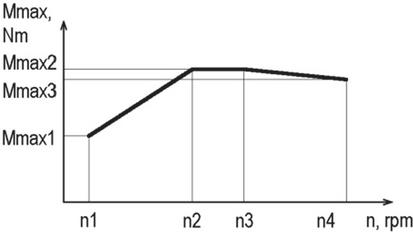
Figure 3 Dependence of the maximum moment Mmax of the diesel engine from the rotational speed n.

The load moment that diesel engine must develop, Nm

$\mathrm{M}\mathrm{d}=\mathrm{M}/{\mathrm{\eta }}_{\mathrm{d}\mathrm{m}}+\mathrm{M}0,$

(3)

where
${\mathrm{\eta }}_{\mathrm{d}\mathrm{m}}$ – diesel engine mechanical efficiency coefficient
M0 – resisting moment of diesel engine at idle run, Nm.

Power available from diesel engine, W

$\text{Pmd}=\text{Md}*\mathrm{o}\mathrm{m}.$

(4)

4.1.2 Model of dynamics

Difference of moment, developed by diesel engine, Nm

$\mathrm{d}\mathrm{M}\mathrm{d}=(\mathrm{\Delta }/\mathrm{T})*((\mathrm{M}\mathrm{m}\mathrm{a}\mathrm{x}/\mathrm{k})*(\mathrm{o}\mathrm{m}0-\mathrm{o}\mathrm{m})-\mathrm{M}\mathrm{d}),$

(5)

where
$\mathrm{\Delta }$ – simulation time step, s
T – time constant, s.

Difference of diesel engine angular speed, rads${\mathrm{}}^{-1}$

$\mathrm{d}\mathrm{o}\mathrm{m}=(\mathrm{\Delta }/\mathrm{J})*(\mathrm{M}\mathrm{d}-\mathrm{M}),$

(6)

where
J – total moment of inertia of diesel engine, hydraulic pump and feeding pump, kgm${\mathrm{}}^2$rad${\mathrm{}}^{-1}$.

4.1.3 Values of parameters

$\mathrm{k}$=$5,\mathrm{n}1$=$1000$ rpm, $\mathrm{n}2$=$1400$ rpm, $\mathrm{n}3$=$1600$ rpm, $\mathrm{n}4$=$2000$ rpm, $\mathrm{M}\mathrm{m}\mathrm{a}\mathrm{x}1=130$ Nm, $\mathrm{M}\mathrm{m}\mathrm{a}\mathrm{x}2=260$ Nm, $\mathrm{M}\mathrm{m}\mathrm{a}\mathrm{x}3=240$ Nm, ${\mathrm{\eta }}_{\mathrm{d}\mathrm{m}}=0.95$, $\mathrm{M}0$=$1$ Nm, $\mathrm{T}$=$0.05$ s, $\mathrm{J}$=$0.33$ kgm${\mathrm{}}^2$ rad${\mathrm{}}^{-1}$.

4.2 Variable Displacement Hydraulic Pump PV2_Q

Variable displacement hydraulic pump is taken as A4VSG (Mannesmann Rexroth AG 2005). The pump consists of body, cylinder block, driving shaft, pistons, swash plate with control lever, swash plate support surface, steering cylinder piston rod and distribution plate.

Inputs: $\mathrm{\alpha }$ – position angle of the pump swash plate, deg, om1 – angular speed, rads${\mathrm{}}^{-1}$, p1 – pressure in pump outlet, Pa, p2 – pressure in pump inlet, Pa, M2 – operating moment of the feeding pump PC, Nm.

Outputs: Q1 – outlet volumetric flow, m${\mathrm{}}^3$s${\mathrm{}}^{-1}$, Q2 – inlet volumetric flow, m${\mathrm{}}^3$s${\mathrm{}}^{-1}$, om2 – angular speed of the feeding pump PC, rads${\mathrm{}}^{-1}$, M1 – total operating moment of pumps, Nm, Fsp –friction force of swash plate against the support surface, reduced to control piston, N, Ppv – power for hydraulic pumps operating, W.

4.2.1 Model of steady state conditions

Working volume of the main pump, m${\mathrm{}}^3$rad${\mathrm{}}^{-1}$

$\mathrm{V}1\mathrm{r}$	$=\mathrm{V}{1}_{\mathrm{m}\mathrm{a}\mathrm{x}}*\mathrm{t}\mathrm{a}\mathrm{n}(\mathrm{\alpha }*\mathrm{\pi }/180))/(\mathrm{t}\mathrm{a}\mathrm{n}({\mathrm{\alpha }}_{\mathrm{m}\mathrm{a}\mathrm{x}}*\mathrm{\pi }/180)$
	$\mathrm{\hspace{1em}}*(1-\mathrm{t}\mathrm{a}\mathrm{n}(\mathrm{\beta }*\mathrm{\pi }/180)),$	(7)

where
V1${\mathrm{}}_{\mathrm{m}\mathrm{a}\mathrm{x}}$ – maximum pump working volume, m${\mathrm{}}^3$rev${\mathrm{}}^{-1}$
$\mathrm{\alpha }$ – position angle of the pump swash plate, deg
${\mathrm{\alpha }}_{\mathrm{m}\mathrm{a}\mathrm{x}}$ – swash plate maximum position angle, deg
$\mathrm{\beta }$ – angle of inclination of the pump pistons, deg.

Hydraulic linear resistances for calculation of volumetric losses at pump pistons RLp, at outer border RL1 and at inner border RL2 of the distribution plate, Nsm${\mathrm{}}^{-5}$

$\mathrm{R}\mathrm{L}\mathrm{p}$	$\mathrm{}=12*\mathrm{\nu }*\mathrm{\rho }*\mathrm{l}*\mathrm{n}\mathrm{p}/2/(\mathrm{\pi }*\mathrm{d}*{\mathrm{h}}^3)/(1+1.5*{(\mathrm{e}\mathrm{x}/\mathrm{h})}^2)$	(8)
$\mathrm{R}\mathrm{L}1$	$\mathrm{}=12*\mathrm{\nu }*\mathrm{\rho }*\mathrm{l}1/(\mathrm{\pi }*\mathrm{d}\mathrm{s}1*\mathrm{h}{1}^3)/2,$	(9)
$\mathrm{R}\mathrm{L}2$	$\mathrm{}=12*\mathrm{\nu }*\mathrm{\rho }*\mathrm{l}2/(\mathrm{\pi }*\mathrm{d}\mathrm{s}2*\mathrm{h}{1}^3)/2,$	(10)

where
$\mathrm{\nu }$ – fluid kinematic viscosity, m${\mathrm{}}^2$s${\mathrm{}}^{-1}$
$\mathrm{\rho }$ – fluid density, kgm${\mathrm{}}^{-3}$
l, l1, l2 – flow gap lengths, m
ds1, ds2 – outer and inner diameter of the distribution plate, m
np – number of pistons,
h1 – flow gap thickness of distribution plate, m
h – pump pistons radial gap, m
ex – eccentricity of pump pistons, m.
Resistance of resistors in parallel connection, Nsm${\mathrm{}}^{-5}$

$\mathrm{R}\mathrm{L}\mathrm{s}=1/(1/\mathrm{R}\mathrm{L}1+1/\mathrm{R}\mathrm{L}2+1/\mathrm{R}\mathrm{l}\mathrm{p}).$

(11)

Pump volumetric flow losses, m${\mathrm{}}^3$s${\mathrm{}}^{-1}$

$\mathrm{Q}\mathrm{v}\mathrm{o}\mathrm{l}=1/\mathrm{R}\mathrm{L}\mathrm{s}*(\mathrm{p}1-\mathrm{p}2)/2.$

(12)

Pump outlet volumetric flow, m${\mathrm{}}^3$s${\mathrm{}}^{-1}$

$\mathrm{Q}1=\mathrm{o}\mathrm{m}1*\mathrm{V}1\mathrm{r}-\mathrm{Q}\mathrm{v}\mathrm{o}\mathrm{l},$

(13)

where
om1 – angular speed of pump, rads${\mathrm{}}^{-1}$.
Total operating moment of pumps, Nm

$\mathrm{M}1=\mathrm{V}1\mathrm{r}*(\mathrm{p}1-\mathrm{p}2)/{\mathrm{\eta }}_{\mathrm{h}\mathrm{m}}+\mathrm{M}01+\mathrm{M}2,$

(14)

where
${\mathrm{\eta }}_{\mathrm{h}\mathrm{m}}$ – hydro-mechanical efficiency coefficient of the main pump

${\mathrm{\eta }}_{\mathrm{h}\mathrm{m}}=1-{\mathrm{k}}_{\mathrm{h}\mathrm{m}}*(\mathrm{p}1-\mathrm{p}2)-{\mathrm{k}}_{\mathrm{o}\mathrm{m}}*\mathrm{o}\mathrm{m}1,$

(15)

where
k${\mathrm{}}_{\mathrm{h}\mathrm{m}}$ – coefficient of dependence of ${\mathrm{\eta }}_{\mathrm{h}\mathrm{m}}$ on pressure drop (p1 $-$ p2), Pa${\mathrm{}}^{-1}$
k${\mathrm{}}_{\mathrm{o}\mathrm{m}}$ – coefficient of dependence of ${\mathrm{\eta }}_{\mathrm{h}\mathrm{m}}$ on om1, srad${\mathrm{}}^{-1}$
M01 – resisting moment at idle run, Nm
M2 – feeding pump operating moment, Nm.

Power used by main pump and feeding pump, W

$\mathrm{P}\mathrm{p}\mathrm{v}=\mathrm{M}1*\mathrm{o}\mathrm{m}1.$

(16)

Friction force of swash plate against the support surface, reduced to control piston, N

$\mathrm{F}\mathrm{s}\mathrm{p}=\mathrm{k}\mathrm{s}\mathrm{p}*\mathrm{A}*\mathrm{n}\mathrm{p}/2*(\mathrm{p}1-\mathrm{p}2)*\mathrm{i},$

(17)

where
ksp – friction coefficient
A – piston area, m${\mathrm{}}^2$ $\mathrm{A}=\mathrm{\pi }*{\mathrm{d}}^2/4$
d – effective diameter of pump piston, m
np – number of pistons
i – force transmission ratio from swash plate to control piston (i $<$ 1).

4.2.2 Model of dynamics

The model of dynamics is similar to the model of steady state conditions except the calculation of volumetric losses.

To calculate volumetric losses of the pump dynamics the inertia of the loss flow, kgm${\mathrm{}}^{-4}$

$\mathrm{L}=\mathrm{\rho }*(\mathrm{l}/\mathrm{A}\mathrm{p}+\mathrm{l}1/\mathrm{A}1+\mathrm{l}2/\mathrm{A}2),$

(18)

where total area of the pistons loss flows, m${\mathrm{}}^2$

$\mathrm{A}\mathrm{p}=(\mathrm{\pi }*\mathrm{d}*\mathrm{h})*\mathrm{n}\mathrm{p}/2*(1+1.5*{(\mathrm{e}\mathrm{x}/\mathrm{h})}^2),$

(19)

areas of the loss flows of distribution plate

$\mathrm{A}1=\mathrm{\pi }*\mathrm{d}\mathrm{s}1*\mathrm{h}1,\mathrm{A}2=\mathrm{\pi }*\mathrm{d}\mathrm{s}2*\mathrm{h}1.$

(20)

Difference of volumetric losses, m${\mathrm{}}^3$/rad

$\mathrm{d}\mathrm{Q}\mathrm{v}\mathrm{o}\mathrm{l}=\mathrm{\Delta }/\mathrm{L}*(\mathrm{p}1-\mathrm{p}2-\mathrm{R}\mathrm{L}\mathrm{s}*\mathrm{Q}\mathrm{v}\mathrm{o}\mathrm{l}).$

(21)

4.2.3 Values of parameters

V1max $=$ 56e–6 m${\mathrm{}}^3$rev${\mathrm{}}^{-1}$ (8.9187e-6 m${\mathrm{}}^3$rad${\mathrm{}}^{-1}$), ${\mathrm{\alpha }}_{\mathrm{m}\mathrm{a}\mathrm{x}}$=$35$ deg (0.6109 rad), ${\mathrm{\alpha }}_{\mathrm{m}\mathrm{i}\mathrm{n}}$=$5$ deg (0.08726 rad), $\mathrm{\beta }=8$ deg (0.1396 rad), $\mathrm{n}\mathrm{p}$=$7$, $\mathrm{l}$=$0.04$ m, $\mathrm{l}1$=$0.01$ m, $\mathrm{l}2$=$0.01$ m, h $=$ 1e–5 m, h1 $=$ 2e–5 m, ex $=$ 1e–5 m, d $=$ 0.0206 m, ds1 $=$ 0.08 m, ds2 $=$ 0.04 m, ksp $=$ 0.03, k${\mathrm{}}_{\mathrm{h}\mathrm{m}}$ $=$ 3e–9 Pa${\mathrm{}}^{-1}$, k${\mathrm{}}_{\mathrm{o}\mathrm{m}}$ $=$ 1e–4 s rad${\mathrm{}}^{-1}$, M0 $=$ 0.1 Nm, i $=$ 0.85.

4.3 Constant Displacement Hydraulic Feeding Pump PC

In the mathematical multi-pole model of the feeding pump the same formulae (see formulae (8)…(15) and (18)…(21)) to those from the model of the main pump are used.

Inputs: om – angular speed, rads${\mathrm{}}^{-1}$, p2 – pressure, Pa.

Outputs: M – driving moment, Nm, Q2 – volumetric flow, m${\mathrm{}}^3$s${\mathrm{}}^{-1}$.

4.3.1 Values of parameters

V $=$ 10e–6 m${\mathrm{}}^3$rev${\mathrm{}}^{-1}$, M0 $=$ 0.02 Nm.

4.4 Variable Displacement Hydraulic Motor MH3

Design of the hydraulic motor is taken similar to the hydraulic pump. Mathematical model of the hydraulic motor is analogous to the model of the hydraulic pump. Some input/output variables are different.

Inputs: $\mathrm{\alpha }$ – position angle of the motor swash plate, deg, M – load moment, Nm, p2 – outlet pressure, Pa.

Outputs: p1 – inlet pressure, Pa, Q2 – volumetric flow, m${\mathrm{}}^3$s${\mathrm{}}^{-1}$, Fsp – Friction force of swash plate against the support surface, reduced to control piston, N, om – angular speed, rads${\mathrm{}}^{-1}$.

Equation for calculating Fsp is similar to hydraulic pump, see (17). Some equations of hydraulic motor are different.

The hydraulic motor inlet pressure, Pa

$\mathrm{p}1=\mathrm{M}1/\mathrm{V}\mathrm{r}/{\mathrm{\eta }}_{\mathrm{h}\mathrm{m}}+\mathrm{M}0/\mathrm{V}\mathrm{r}+\mathrm{p}2,$

(22)

volumetric flow, m${\mathrm{}}^3$s${\mathrm{}}^{-1}$

$\mathrm{Q}2=\mathrm{Q}1-\mathrm{Q}\mathrm{v}\mathrm{o}\mathrm{l},$

(23)

angular speed, rads${\mathrm{}}^{-1}$

$\mathrm{o}\mathrm{m}=\mathrm{Q}2/\mathrm{V}\mathrm{r}.$

(24)

The model is used for both steady state conditions and dynamics considering that the moment of inertia of hydraulic motor rotor is added to speed reducer.

4.4.1 Values of parameters

V $=$ 54.8e-6 m${\mathrm{}}^3$rev${\mathrm{}}^{-1}$, h $=$ 3e-5 m, l $=$ 0.03 m, ${\mathrm{\alpha }}_{\mathrm{m}\mathrm{i}\mathrm{n}}$ $=$ 12 deg, the remaining parameters are the same as for the hydraulic pump (see 4.2.3).

4.5 Control Cylinders SPP_PIS and SPM_PIS

Control cylinders SPP_PIS and SPM_PIS are used for automatic control of the hydraulic pump and the hydraulic motor correspondingly. The cylinders are of the same design, have the same parameters and are described by the similar multi-pole model. Piston in control cylinder moves the swash plate of the pump or the motor depending on the input and output pressure of the pump or motor.

Inputs: p2 – pressure in pump or motor inlet, Pa, p1 – pressure in pump or motor outlet, Pa, Fsp –friction force of the swash plate support surface reduced to the control piston, N.

Outputs: y – control piston displacement, m, $\mathrm{\alpha }$ – position angle of the pump or motor swash plate, deg, Q1, Q2 – volumetric flows, m${\mathrm{}}^3$s${\mathrm{}}^{-1}$.

4.5.1 Model of steady state conditions

Effective areas of the control pistons, m${\mathrm{}}^2$

$\mathrm{A}1=\mathrm{\pi }*(\mathrm{d}\mathrm{c}{\mathrm{y}}^2-\mathrm{d}{1}^2)/4,\mathrm{A}2=\mathrm{\pi }*(\mathrm{d}\mathrm{c}{\mathrm{y}}^2-\mathrm{d}{2}^2)/4,$

(25)

where
dcy – inner diameter of control cylinder, m
d1, d2 – diameters of control piston rods, m.
Friction force reduced to the control piston, N

$\mathrm{F}\mathrm{f}\mathrm{r}=\mathrm{F}\mathrm{f}\mathrm{r}0+\mathrm{k}\mathrm{f}\mathrm{r}*(\mathrm{p}2-\mathrm{p}1),$

(26)

where
Ffr0 – friction force at idle run, N
kfr – coefficient of dependence of friction force on pressure drop (p1 – p2),
m${\mathrm{}}^2$.

Force of spring preliminary deformation, N

$\mathrm{F}0=\mathrm{y}0*\mathrm{c},$

(27)

where
y0 – preliminary deformation of the spring, m
c – stiffness of the control piston spring, Nm${\mathrm{}}^{-1}$

$\mathrm{c}=\mathrm{G}*{\mathrm{d}}^4/(8*\mathrm{n}\mathrm{s}*{\mathrm{D}}^3),$

(28)

where
G – shear modulus, Nm${\mathrm{}}^{-2}$
d – diameter of spring wire, m
D – diameter of spring, m
ns – number of turns of the spring.
Force acting on the control valve, m

$\mathrm{F}\mathrm{y}=\mathrm{p}2*\mathrm{A}2-\mathrm{p}1*\mathrm{A}1-\mathrm{F}\mathrm{s}\mathrm{p}-\mathrm{F}\mathrm{f}\mathrm{r}+\mathrm{F}0.$

(29)

Displacement of the control piston, m

$\mathrm{y}=\mathrm{F}\mathrm{y}/\mathrm{c}.$

(30)

Position angle of the hydraulic pump swash plate, deg

$\mathrm{\alpha }={\mathrm{\alpha }}_{\mathrm{m}\mathrm{a}\mathrm{x}}-\mathrm{a}\mathrm{t}\mathrm{a}\mathrm{n}(\mathrm{y}/(\mathrm{r}*\mathrm{i})*(180/\mathrm{\pi })),$

(31)

position angle of the hydraulic motor swash plate, deg

$\mathrm{\alpha }=\mathrm{a}\mathrm{t}\mathrm{a}\mathrm{n}(\mathrm{y}/(\mathrm{r}*\mathrm{i})*(180/\mathrm{\pi })),$

(32)

where
r – distance between control piston rod and swash plate turning axis, m
i – force transmission ratio from the swash plate to control piston (or displacement transmission from the control piston to swash plate) (i $<$ 1).

Volumetric flows

$\mathrm{Q}1=\mathrm{Q}2=0.$

(33)

4.5.2 Model of dynamics

Friction force, N

$\mathrm{F}\mathrm{f}\mathrm{r}=(\mathrm{F}\mathrm{f}\mathrm{r}0+\mathrm{k}\mathrm{f}\mathrm{r}*(\mathrm{p}2-\mathrm{p}1))*\mathrm{s}\mathrm{i}\mathrm{g}\mathrm{n}\mathrm{v}(\mathrm{v},{\mathrm{v}}_{\mathrm{l}\mathrm{i}\mathrm{n}}),$

(34)

where
signv – function characterising dependence from the direction of movement, velocity v of the control piston and the range of the linear effect of velocity ${\mathrm{v}}_{\mathrm{l}\mathrm{i}\mathrm{n}}$.

Difference of piston velocity, ms${\mathrm{}}^{-1}$

$\mathrm{d}\mathrm{v}=(\mathrm{\Delta }/\mathrm{m})*(\mathrm{F}\mathrm{y}-\mathrm{y}*\mathrm{c}-\mathrm{F}\mathrm{f}\mathrm{r}-\mathrm{h}*\mathrm{v}),$

(35)

where
$\mathrm{\Delta }$ – simulation time step, s
m – sum of mass of piston with pump swash plate and 1/3 mass of spring, kg
h – damping coefficient, Nsm${\mathrm{}}^{-1}$.

Difference of piston displacement, m

$\mathrm{d}\mathrm{y}=\mathrm{\Delta }*\mathrm{v},$

(36)

volumetric flows, m${\mathrm{}}^3$s${\mathrm{}}^{-1}$

$\mathrm{Q}1=-\mathrm{A}1*\mathrm{v},\mathrm{Q}2=\mathrm{A}2*\mathrm{v}.$

(37)

4.5.3 Values of parameters

dcy $=$ 0.04 m, dro1 $=$ 0.02 m, dro2 $=$ 0.035 m, r $=$ 0.08 m, Ffr0 $=$ 30 N, kfr $=$ 5e–7 m${\mathrm{}}^2$, y0 $=$ 0.001 m, G $=$ 8e11 Nm${\mathrm{}}^{-2}$, d $=$ 0.0034 m, D $=$ 0.024 m, ns $=$ 5, mv $=$ 0.5 kg, ms $=$ 0,06 kg, h=200 Nsm${\mathrm{}}^{-1}$, ${\mathrm{\alpha }}_{\mathrm{m}\mathrm{i}\mathrm{n}}$ $=$ 5 deg (for SPP_PIS), ${\mathrm{\alpha }}_{\mathrm{m}\mathrm{i}\mathrm{n}}$ $=$ 12 deg (for SPM_PIS), ${\mathrm{\alpha }}_{\mathrm{m}\mathrm{a}\mathrm{x}}$ $=$ 35 deg, i $=$  0.85, ${\mathrm{v}}_{\mathrm{l}\mathrm{i}\mathrm{n}}=1$e-7 ms${\mathrm{}}^{-1}$.

4.6 Pressure Relief Valves PRV1 and PRV2

Pressure relief valves are used to ensure the constant pressure under steady state conditions for feeding (PRV1) and for flushing (PRV2) of the closed-loop transmission. Both valves are of similar construction. The pressure relief valve is considered to consist of three components: poppet valve, flow opening of poppet valve and spring retainer (Harf and Grossschmidt 2014).

4.6.1 Poppet valve VPC_pl_rel

4.6.1.1 Model of steady state conditions

Inputs: y – displacement of the poppet valve, m, dp – pressure drop in flow opening, Pa, p2 – pressure acting to the spring retainer, Pa, p3 – outlet pressure; Pa, fV0 – preliminary deformation of the spring, m.

Outputs: p1 – inlet pressure, Pa, Q1, Q2 – volumetric flows.

Pressure, Pa

$\mathrm{p}1=\mathrm{F}1/\mathrm{A},$

(38)

where
F1 – hydraulic force to surface A necessary for opening the valve, N

$\mathrm{F}1$	$\mathrm{}=(\mathrm{y}+\mathrm{f}\mathrm{V}0)*\mathrm{c}-\mathrm{F}\mathrm{r}+\mathrm{F}2-\mathrm{F}\mathrm{j}-\mathrm{F}\mathrm{f}\mathrm{r}-\mathrm{\pi }$
	$\mathrm{\hspace{1em}}*(\mathrm{d}{2}^2-\mathrm{d}{1}^2)/8*\mathrm{d}\mathrm{p}*\mathrm{s}\mathrm{i}\mathrm{n}(\mathrm{\beta }*\mathrm{\pi }/180),$	(39)

where
c – stiffness of the pressure relief valve spring, Nm${\mathrm{}}^{-1}$, see (28)
Fr – force acting to the spring retainer in the valve opening direction, N

$\mathrm{F}\mathrm{r}=\mathrm{\pi }*(\mathrm{d}{\mathrm{r}}^2-\mathrm{d}{2}^2)/4*\mathrm{p}2/2$

(40)

dr – diameter of the spring retainer, m
d2 – larger diameter of the poppet, m
F2 – force acting in the valve closing direction on the spring retainer, N

$\mathrm{F}2=\mathrm{\pi }*\mathrm{d}{\mathrm{r}}^2*\mathrm{p}3/4$

(41)

Fj – force of fluid jet, acting in the valve opening direction, N

$\mathrm{F}\mathrm{j}$	$\mathrm{}=2*\mathrm{d}\mathrm{p}*\mathrm{\mu }*\mathrm{\pi }*((\mathrm{d}1+\mathrm{d}2)/2+\mathrm{y}*\mathrm{t}\mathrm{a}\mathrm{n}(\mathrm{\beta }*\mathrm{\pi }/180))$
	$\mathrm{\hspace{1em}}*\mathrm{y}*\mathrm{s}\mathrm{i}\mathrm{n}(\mathrm{\beta }*\mathrm{\pi }/180)*\mathrm{c}\mathrm{o}\mathrm{s}(\mathrm{\gamma }*\mathrm{\pi }/180),$	(42)

where
$\mathrm{\mu }$ – flow coefficient
d1, d2 – smaller and larger diameter of the poppet, m
$\mathrm{\beta }$ – inclination angle of the valve poppet, deg
$\mathrm{\gamma }$ – angle between the fluid jet and the valve axis, deg.
Ffr – friction force in the opposite direction of the valve opening, N

$\mathrm{F}\mathrm{f}\mathrm{r}=(\mathrm{F}\mathrm{f}\mathrm{r}0+\mathrm{k}\mathrm{f}\mathrm{r}*\mathrm{d}\mathrm{p}),$

(43)

where
Ffr0 – permanent part of the friction force, N
kfr – coefficient of dependence of friction force on pressure drop dp, m${\mathrm{}}^2$.
A – pressure relief valve effective area, m${\mathrm{}}^2$

$\mathrm{A}=\mathrm{\pi }*\mathrm{d}{1}^2/4.$

(44)

Volumetric flows

$\mathrm{Q}1=\mathrm{Q}2=0.$

(45)

4.6.1.2 Model of dynamics

Inputs: p1, p2, p3 – pressures, Pa, dp – pressure drop in flow opening, Pa, fV0 – preliminary deformation of the spring, m

Outputs: y – displacement of the poppet valve, m, Q1, Q2 – volumetric flows, m${\mathrm{}}^3$s${\mathrm{}}^{-1}$

Difference of valve velocity, m/s

$\mathrm{d}\mathrm{v}=(\mathrm{\Delta }/\mathrm{m})*(\mathrm{F}1+\mathrm{F}\mathrm{r}-\mathrm{F}2+\mathrm{F}\mathrm{j}-(\mathrm{y}+\mathrm{f}\mathrm{V}0)*\mathrm{c}+\mathrm{F}\mathrm{f}\mathrm{r}-\mathrm{h}*\mathrm{v}),$

(46)

where
$\mathrm{\Delta }$ – simulation time step, s
m – sum of valve mass mv and 1/3 of spring mass, kg
F1– lifting hydraulic force, N

$\mathrm{F}1=\mathrm{p}1*\mathrm{A}+\mathrm{\pi }*(\mathrm{d}{2}^2-\mathrm{d}{1}^2)/8*\mathrm{d}\mathrm{p}*\mathrm{s}\mathrm{i}\mathrm{n}(\mathrm{\beta }*\mathrm{\pi }/180)$

(47)

displacement of the poppet valve, m

$\mathrm{y}=(\mathrm{F}1+\mathrm{F}\mathrm{r}-\mathrm{F}2+\mathrm{F}\mathrm{j}-\mathrm{F}\mathrm{f}\mathrm{r}-\mathrm{h}*\mathrm{v})/\mathrm{c}-\mathrm{f}\mathrm{V}0,$

(48)

where friction force in the opposite direction of the valve opening, N

$\mathrm{F}\mathrm{f}\mathrm{r}=(\mathrm{F}\mathrm{f}\mathrm{r}0+\mathrm{k}\mathrm{f}\mathrm{r}*\mathrm{d}\mathrm{p})*\mathrm{s}\mathrm{i}\mathrm{g}\mathrm{n}\mathrm{v}(\mathrm{v},{\mathrm{v}}_{\mathrm{l}\mathrm{i}\mathrm{n}}),$

(49)

where
signv – see formula (34)
h – damping coefficient, Nsm${\mathrm{}}^{-1}$
v – poppet valve velocity, ms${\mathrm{}}^{-1}$.

Difference of poppet valve displacement

$\mathrm{d}\mathrm{y}=\mathrm{\Delta }*\mathrm{v}.$

(50)

Volumetric flows, m${\mathrm{}}^3$s${\mathrm{}}^{-1}$

$\mathrm{Q}1=-\mathrm{v}*\mathrm{A},\mathrm{Q}2=\mathrm{v}*\mathrm{A}.$

(51)

4.6.1.3 Values of parameters

d1 $=$ 0.004 m, d2 $=$ 0.005 m, dr $=$ 0.02 m, $\mathrm{\mu }$ $=$ 0.8, $\mathrm{\beta }$ $=$ 15 deg, $\mathrm{\gamma }$ $=$ 45 deg, d $=$ 0.0009 m, D $=$ 0.014 m, ns $=$ 8, G $=$ 8e11 Nm${\mathrm{}}^{-2}$, Ffr0 $=$ 0, kfr $=$ 1e$-$8 m${\mathrm{}}^2$, m $=$ 0.04 kg, h $=$ 250 Nsm${\mathrm{}}^{-1}$, v${}_{\mathrm{l}\mathrm{i}\mathrm{n}}=1$e-7 ms${\mathrm{}}^{-1}$, fV0 $=$ 0.005 m (for feeding pressure valve), fV0 $=$ 0.0022 (for flushing pressure valve), p3 $=$ 0.

4.6.2 Flow opening of poppet valve

4.6.2.1 Model of steady state conditions RPC_rel_st

Inputs: Q1 – volumetric flow, m${\mathrm{}}^3$s${\mathrm{}}^{-1}$, p1, p2 – pressures, Pa

Outputs: y – displacement of the poppet valve, m, dp – pressure drop of flow opening, Pa,
Q2 – volumetric flow, m${\mathrm{}}^3$s${\mathrm{}}^{-1}$.

The area of the flow opening, m${\mathrm{}}^2$

$\mathrm{A}\mathrm{d}=\mathrm{Q}1/\mathrm{\mu }/{(2/\mathrm{\rho }*(\mathrm{p}1-\mathrm{p}2))}^{1/2}),$

(52)

where
$\mathrm{\mu }$ – flow coefficient
$\mathrm{\rho }$ – fluid density, kgm${\mathrm{}}^{-3}$.
Displacement of the poppet valve, m

$\mathrm{y}=\mathrm{A}\mathrm{d}/((\mathrm{\pi }*((\mathrm{d}1+\mathrm{d}2)/2)+\mathrm{y}*\mathrm{t}\mathrm{a}\mathrm{n}(\mathrm{\beta }*\mathrm{\pi }/180))*\mathrm{s}\mathrm{i}\mathrm{n}(\mathrm{\beta }*\mathrm{\pi }/180)),$

(53)

where
d1, d2 – smaller and larger diameter of the poppet valve, m
$\mathrm{\beta }$ – inclination angle of the poppet, deg.
Pressure drop in the flow opening, Pa

$\mathrm{d}\mathrm{p}=\mathrm{p}1-\mathrm{p}2.$

(54)

Volumetric flow, m${\mathrm{}}^3$s${\mathrm{}}^{-1}$

$\mathrm{Q}2=\mathrm{Q}1=0.$

(55)

Models of dynamics of flow openings of feeding valve and flushing valve are different.

4.6.2.2 Model of dynamics of feeding valve flow opening RPC_rel_dyn

Inputs: y – displacement of the poppet valve, m, Q1 – volumetric flow, m${\mathrm{}}^3$s${\mathrm{}}^{-1}$, p2 – pressure, Pa

Outputs: p1 – pressure, Pa, dp – pressure drop in the flow opening, Pa, Q2 – volumetric flow, m${\mathrm{}}^3$s${\mathrm{}}^{-1}$

Area of the valve flow opening, m${\mathrm{}}^2$

$\mathrm{A}\mathrm{d}=\mathrm{\pi }*((\mathrm{d}1+\mathrm{d}2)/2+\mathrm{y}*\mathrm{t}\mathrm{a}\mathrm{n}(\mathrm{\beta }*\mathrm{\pi }/180))*\mathrm{y}*\mathrm{s}\mathrm{i}\mathrm{n}(\mathrm{\beta }*\mathrm{\pi }/180).$

(56)

Pressure, Pa

$\mathrm{p}1=\mathrm{p}2+{(\mathrm{Q}1/(\mathrm{\mu }*\mathrm{A}\mathrm{d}))}^2*\mathrm{\rho }/2.$

(57)

Pressure drop, Pa

$\mathrm{d}\mathrm{p}=\mathrm{p}1-\mathrm{p}2.$

(58)

Volumetric flow, m${\mathrm{}}^3$s${\mathrm{}}^{-1}$

$\mathrm{Q}2=\mathrm{Q}1.$

(59)

4.6.2.3 Model of dynamics of flushing valve flow opening RPPC

Inputs: y – displacement of the poppet valve, m, p1, p2 – pressures, Pa

Outputs: Q1, Q2 – volumetric flows, m${\mathrm{}}^3$s${\mathrm{}}^{-1}$, dp – pressure drop of the flow opening, Pa

Area of the flow opening, m${\mathrm{}}^2$

$\mathrm{A}\mathrm{d}=\mathrm{\pi }*((\mathrm{d}1+\mathrm{d}2)/2+\mathrm{y}*\mathrm{t}\mathrm{a}\mathrm{n}(\mathrm{\beta }*\mathrm{\pi }/180))*\mathrm{y}*\mathrm{s}\mathrm{i}\mathrm{n}(\mathrm{\beta }*\mathrm{\pi }/180).$

(60)

Volumetric flows, m${\mathrm{}}^3$s${\mathrm{}}^{-1}$

$\mathrm{Q}1$	$\mathrm{}=\mathrm{\mu }*\mathrm{A}\mathrm{d}*{(2/\mathrm{\rho }*(\mathrm{p}1-\mathrm{p}2))}^{1/2}$	(61)
$\mathrm{Q}2$	$\mathrm{}=\mathrm{Q}1.$	(62)

Pressure drop of the flow opening, Pa

$\mathrm{d}\mathrm{p}=\mathrm{p}1-\mathrm{p}2.$

(63)

4.6.2.4 Values of parameters

d1 $=$ 0.004 m, d2 $=$ 0.005 m, $\mathrm{\mu }$ $=$ 0.8, $\mathrm{\beta }$ $=$ 15 deg.

4.6.3 Spring retainer ResH_rad

The spring retainer has a radial slot through the poppet valve body, which operates as an additional resistor in steady state conditions mode and as a vibration damper in dynamics.

Inputs: y – displacement of the poppet valve, m, Q1 – volumetric flow, m${\mathrm{}}^3$s${\mathrm{}}^{-1}$, p2 – pressure, Pa.

Outputs: p1 – pressure, Pa, Q2 – volumetric flow, m${\mathrm{}}^3$s${\mathrm{}}^{-1}$.

4.6.3.1 Model of steady state conditions and dynamics

Pressure in outlet of circular radial slot, Pa

$\mathrm{p}1=\mathrm{p}2+(\mathrm{R}\mathrm{L}+\mathrm{R}\mathrm{T}*\mathrm{a}\mathrm{b}\mathrm{s}(\mathrm{Q}1))*\mathrm{Q}1,$

(64)

where

$\mathrm{R}\mathrm{L}$	$\mathrm{}=12*\mathrm{\nu }*\mathrm{\rho }*\mathrm{l}/(\mathrm{\pi }*\mathrm{d}\mathrm{d}*\mathrm{y}{\mathrm{s}}^3)$
$\mathrm{R}\mathrm{T}$	$\mathrm{}=\mathrm{\rho }/2/{(\mathrm{\mu }*\mathrm{\pi }*\mathrm{d}\mathrm{d}*\mathrm{y}\mathrm{s})}^2$
$\mathrm{l}$	$\mathrm{}=(\mathrm{d}\mathrm{r}-\mathrm{d}1)/2$
$\mathrm{d}\mathrm{d}$	$\mathrm{}=(\mathrm{d}\mathrm{r}+\mathrm{d}1)/2$
$\mathrm{y}\mathrm{s}$	$\mathrm{}=\mathrm{f}\mathrm{V}0+\mathrm{y}$

dr – diameter of spring retainer, m.

4.6.3.2 Values of parameters

dr $=$ 0.02 m, p2 $=$ 0.

4.7 Speed reducer TrrH

Speed reducer decreases the angular speed and increases the moment to be developed by the transmission.

Inputs: om1 – inlet angular speed, rads${\mathrm{}}^{-1}$, M2 – outlet moment, Nm.

Outputs: om2 – outlet angular speed, rads${\mathrm{}}^{-1}$, M1 – inlet moment, Nm.

4.7.1 Model of steady state conditions

Moment at inlet, Nm

$\mathrm{M}1=\mathrm{M}2*\mathrm{i}/{\mathrm{\eta }}_{\mathrm{m}}+\mathrm{M}10+\mathrm{h}\mathrm{o}\mathrm{m}*(\mathrm{o}\mathrm{m}1*\mathrm{i}-\mathrm{o}\mathrm{m}2),$

(65)

where
i – transfer factor
${\mathrm{\eta }}_{\mathrm{m}}$ – mechanical efficiency coefficient
M10 – resisting moment at idle run, Nm
hom – damping coefficient according to angular speed (om1*i – om2), Nmsrad${\mathrm{}}^{-1}$.
Angular speed at outlet, rads${\mathrm{}}^{-1}$

$\mathrm{o}\mathrm{m}2=\mathrm{o}\mathrm{m}1*\mathrm{i}.$

(66)

4.7.2 Model of dynamics

Difference moment at inlet, Nm

$\mathrm{d}\mathrm{M}1=(\mathrm{\Delta }/\mathrm{e})*((\mathrm{o}\mathrm{m}1*\mathrm{i}-\mathrm{o}\mathrm{m}2)-\mathrm{h}\mathrm{m}*(\mathrm{M}1-\mathrm{M}2*\mathrm{i}/{\mathrm{\eta }}_{\mathrm{m}}-\mathrm{M}10)),$

(67)

where
$\mathrm{\Delta }$ – simulation time step, s
e – torsion elasticity, radN${\mathrm{}}^{-1}$ m${\mathrm{}}^{-1}$.
Difference angular speed at outlet, rads${\mathrm{}}^{-1}$

$\mathrm{d}\mathrm{o}\mathrm{m}2=(\mathrm{\Delta }/\mathrm{J})*(\mathrm{M}1-\mathrm{M}2*\mathrm{i}/{\mathrm{\eta }}_{\mathrm{m}}-\mathrm{M}10),$

(68)

where
J – moment of inertia, kgm${\mathrm{}}^2$rad${\mathrm{}}^{-1}$.

4.7.3 Values of parameters

i $=$ 0.2, ${\mathrm{\eta }}_{\mathrm{m}}$ $=$ 0.95, M10 $=$ 0.1 Nm, e $=$ 3e-5 radN${\mathrm{}}^{-1}$ m${\mathrm{}}^{-1}$, J $=$ 0.002 kgm${\mathrm{}}^2$rad${\mathrm{}}^{-1}$.

4.8 Rotary Actuator AcrH

Rotary actuator is a rotating working mechanism.

Inputs: om1 – angular speed at inlet, rads${\mathrm{}}^{-1}$, M2 – moment at outlet, Nm.

Outputs: om2 – angular speed at outlet, rads${\mathrm{}}^{-1}$, M1 – moment at inlet, Nm, Pac – power at outlet, W.

4.8.1 Model of steady state conditions

Moment at inlet, Nm

$\mathrm{M}1=\mathrm{M}2/{\mathrm{\eta }}_{\mathrm{m}}+\mathrm{M}10,$

(69)

where
${\mathrm{\eta }}_{\mathrm{m}}$ – mechanical efficiency coefficient
M10 – resisting moment at idle run, Nm.
Angular speed at outlet, rads${\mathrm{}}^{-1}$

$\mathrm{o}\mathrm{m}2=\mathrm{o}\mathrm{m}1.$

(70)

Power at outlet, W

$\mathrm{P}\mathrm{a}\mathrm{c}=\mathrm{M}2*\mathrm{o}\mathrm{m}2.$

(71)

4.8.2 Model of dynamics

Difference of moment at inlet, Nm

$\mathrm{d}\mathrm{M}1=(\mathrm{\Delta }/\mathrm{e})*(\mathrm{o}\mathrm{m}1-\mathrm{o}\mathrm{m}2-\mathrm{h}\mathrm{M}*(\mathrm{M}1-\mathrm{M}2/{\mathrm{\eta }}_{\mathrm{m}}-\mathrm{M}10)),$

(72)

where
$\mathrm{\Delta }$ – simulation time step, s
e – torsion elasticity, radN${\mathrm{}}^{-1}$m${\mathrm{}}^{-1}$
M10 – resisting moment at idle run, Nm
hM – damping constant according to the difference of moments $(\mathrm{M}1-\mathrm{M}2/{\mathrm{\eta }}_{\mathrm{m}}-\mathrm{M}10)$,
radN${\mathrm{}}^{-1}$m${\mathrm{}}^{-1}$s${\mathrm{}}^{-1}$
Difference of angular speed at outlet, rads${\mathrm{}}^{-1}$

$\mathrm{d}\mathrm{o}\mathrm{m}2=(\mathrm{\Delta }/\mathrm{J})*(\mathrm{M}1-\mathrm{M}2/{\mathrm{\eta }}_{\mathrm{m}}-\mathrm{M}10-\mathrm{h}\mathrm{o}\mathrm{m}*(\mathrm{o}\mathrm{m}1-\mathrm{o}\mathrm{m}2)),$

(73)

where
J – moment of inertia, kgm${\mathrm{}}^2$rad${\mathrm{}}^{-1}$
${\mathrm{\eta }}_{\mathrm{m}}$ – mechanical efficiency coefficient
hom – damping constant according to difference of angular speed (om1 – om2),
Nmsrad${\mathrm{}}^{-1}$.

4.8.3 Values of parameters

${\mathrm{\eta }}_{\mathrm{m}}$ $=$ 0.95, M10 $=$ 1 Nm, e $=$ 3e–5 radN${\mathrm{}}^{-1}$m${\mathrm{}}^{-1}$, J $=$ 1 kgm${\mathrm{}}^2$rad${\mathrm{}}^{-1}$, hom =0.01 Nmsrad${\mathrm{}}^{-1}$, hM $=$ 0.15 radN${\mathrm{}}^{-1}$m${\mathrm{}}^{-1}$s${\mathrm{}}^{-1}$.

4.9 Filter ResH_FIL_Q, Heater ResH_HE_Q (or Cooler ResH_CO_Q)

Mathematical model of laminar flow is used for both steady state conditions and dynamics.

Inputs: Q1 – volumetric flow, m${\mathrm{}}^3$s${\mathrm{}}^{-1}$, p2 – pressure, Pa

Outputs: p1 – pressure, Pa, Q2 – volumetric flow, m${\mathrm{}}^3$s${\mathrm{}}^{-1}$ Pressure, Pa

$\mathrm{p}1=\mathrm{p}2+\mathrm{R}\mathrm{L}*\mathrm{Q}1,$

(74)

where

RL – resistance at laminar flow, Pas m${\mathrm{}}^{-3}$
RL $=$ pn/Qn,	(75)
pn – nominal pressure drop, Pa
Qn – nominal volumetric flow, m${\mathrm{}}^3$s${\mathrm{}}^{-1}$.

Volumetric flow, m${\mathrm{}}^3$s${\mathrm{}}^{-1}$

$\mathrm{Q}2=\mathrm{Q}1.$

(76)

4.9.1 Values of parameters

pn $=$ 2e5 Pa, Qn =1e–3 m${\mathrm{}}^3$s${\mathrm{}}^{-1}$.

4.10 Directional valve ResH_DV_Q

Mathematical model of turbulent flow is used for both steady state conditions and dynamics.

Inputs: Q1 – volumetric flow, m${\mathrm{}}^3$s${\mathrm{}}^{-1}$, p2 – pressure, Pa

Outputs: p1 – pressure, Pa, Q2 – volumetric flow, m${\mathrm{}}^3$s${\mathrm{}}^{-1}$ Pressure, Pa

$\mathrm{p}1=\mathrm{p}2+\mathrm{R}\mathrm{T}*\mathrm{Q}{1}^2,$

(77)

where

RT – resistance at turbulent flow, Pa s${\mathrm{}}^2$m${\mathrm{}}^{-6}$
RT $=$ pn/Qn${\mathrm{}}^2$,	(78)
pn – nominal pressure drop, Pa
Qn – nominal volumetric flow, m${\mathrm{}}^3$s${\mathrm{}}^{-1}$.

Volumetric flow, m${\mathrm{}}^3$s${\mathrm{}}^{-1}$

$\mathrm{Q}2=\mathrm{Q}1.$

(79)

4.10.1 Values of parameters

pn $=$ 1e5 Pa, Qn =1e–3 m${\mathrm{}}^3$s${\mathrm{}}^{-1}$.

4.11 Check valve ResG_CV

Pressure drop in check valve is determined by spring force and depends on the design of the valve.

Inputs: Q2 – volumetric flow, m${\mathrm{}}^3$s${\mathrm{}}^{-1}$, p1 – pressure, Pa

Outputs: p2 – pressure, Pa, Q1 – volumetric flow, m${\mathrm{}}^3$s${\mathrm{}}^{-1}$ Pressure, Pa

$\mathrm{p}2=\mathrm{p}1-\mathrm{d}\mathrm{p}.$

(80)

Volumetric flow, m${\mathrm{}}^3$s${\mathrm{}}^{-1}$

$\mathrm{Q}1=\mathrm{Q}2.$

(81)

4.11.1 Values of parameters

dp $=$ 1e5 Pa.

4.12 Efficiency coefficient calculator EC

Efficiency coefficient is calculated for steady state conditions.

Inputs: Pmd – power used from diesel engine, W, Ppv – outlet power of the pump, W, Pac – outlet power of the actuator, W.

Outputs: eHS – efficiency coefficient of the hydraulic rotary transmission without engine, eG – efficiency coefficient of the hydraulic rotary transmission with engine.

Efficiency coefficient of the hydraulic part

$\mathrm{e}\mathrm{H}\mathrm{S}=\mathrm{P}\mathrm{a}\mathrm{c}/\mathrm{P}\mathrm{p}\mathrm{v}.$

(82)

Efficiency coefficient of the whole transmission

$\mathrm{e}\mathrm{G}=\mathrm{P}\mathrm{a}\mathrm{c}/\mathrm{P}\mathrm{m}\mathrm{d}.$

(83)

4.13 Hydraulic Interface Elements IEH

Hydraulic interface elements express:

• equality of output pressures, if pressure of one pole is given as input,

• equation of continuity of volumetric flows, for example

$\mathrm{Q}4=\mathrm{Q}3-\mathrm{Q}2+\mathrm{Q}1\mathrm{i}\mathrm{n}\mathrm{I}\mathrm{E}\mathrm{H}6\mathrm{\_}3-1\mathrm{\_}1.$

4.14 Other Models

Models of tubes, hydraulic resistors and physical properties of fluids are described in (Grossschmidt and Harf 2009a, 2009b, 2010). Parameters of hydraulic resistors ResG are as follows: l $=$ 0.001 m, d $=$ 0.0009 m (at SPP_PIS and SPM_PIS), d $=$ 0.0008 m (at feeding and flushing pressure valve).

Models of hydraulic hoses HoseH_pandHoseH_Q are presented in (Grossschmidt and Harf 2018). Suffix p or Q in the model HoseH denotes that outputs (pressure p or volumetric flow Q) are calculated using iteration. Values of main parameters of hoses: inner diameter d $=$ 0.02 m, length l $=$ 2 m.

5 Simulation Environment

CoCoViLa is a tool for model-based software development with a visual language support. It uses automatic synthesis of programs for translating declarative specifications of simulation problems into executable code. Automatic program synthesis in CoCoViLa involves following stages: specification parsing, problem creation, planning, code generation and compilation. Using a visual simulation environment like CoCoViLa enables us to describe multi-pole models graphically which facilitates the model development. Automatic synthesis of the calculation algorithms allows focusing on designing models of fluid power systems instead of constructing and solving simulation algorithms.

CoCoViLa is developed as an open-source software, its extensions can be written in Java and included into simulation packages. CoCoViLa is implemented in the Institute of Cybernetics at the Tallinn University of Technology. The CoCoViLa environment is platform-independent and free.

In order to use mathematical multi-pole models in simulations all the formulae of models must be transferred into executable Java functions.

6 Simulation Process Organization

Using visual specifications of described multi-pole models of fluid power system components one can compose models of various fluid power systems for simulating both steady state conditions and dynamic responses.

Principles of simulation process organisation have been considered in (Grossschmidt and Harf 2016). A brief review of principles of simulation process organisation is presented as follows.

When simulating steady state conditions fluid power system behaviour is simulated depending on different values of inputs. Number of calculation points must be specified.

When simulating dynamic behaviour, transient responses in certain points of the system caused by applied disturbances are calculated. Disturbances are considered as changes of inputs of the rotary transmission (load moments, diesel engine rotational speed, etc.).

Steady state and dynamic computing processes are organized by the corresponding process managers (static Process, dynamic Process). To follow the system behaviour, the concept of state is invoked. State variables are introduced for a component in order to characterize its behaviour at the current simulation step.

A simulation task requires sequential computing states until some satisfying final state is reached. For example number of computing steps, simulation time, etc. can be conditions to be satisfied.

A final state can be computed from a given initial state if a function exists that calculates the next state from known previous states. This function is to be constructed automatically by the CoCoViLa program synthesizer.

When calculating next state from previous states loop dependencies between poles of component models may occur. A special technique is used for calculating variables in loop dependences that may appear when multi-pole models of components are connected together. One variable in each loop is split and iteratively recomputed to find its value satisfying the loop dependency.

State variables and split variables must be described in component models. When building a particular simulation task model and performing simulations, state variables and split variables are used automatically by the CoCoViLa program synthesizer if needed.

When building up a simulation task scheme all the parameters of components must be provided with values. Initial values of state variables and variables requiring iterations characterize the model in the beginning of the simulation. Specifying precise initial values is not critical for steady state conditions. Approximate initial values must be set. For dynamics setting initial conditions is critical to guarantee reliable transient responses calculated. Trustful initial conditions can be obtained only as a result of calculations of transient responses in the case of zero disturbances which must be performed as a separate simulation.

Maximum number of iterations, adjusting factor for iterations, allowed absolute and relative errors are to be specified for calculating variables in loops.

The graphs generated during the simulation allow evaluate the results in whatever point of interest of the rotary transmission.

Physical properties of working fluid (density $\mathrm{\rho }$, kinematic viscosity $\mathrm{\nu }$ and compressibility factor $\mathrm{\beta }$) are calculated at each simulation step depending on the average of input and output pressure in the component. In all the simulations below the hydraulic fluid HLP46 is used. The initial values of physical properties of fluid HLP46 at zero pressure and at temperature 40${\mathrm{}}^{\mathrm{o}}$C are: density $\mathrm{\rho }$ $=$ 873 kgm${\mathrm{}}^{-3}$, viscosity $\mathrm{\nu }$ $=$ 46e–6 m${\mathrm{}}^2$s${\mathrm{}}^{-1}$, compressibility factor $\mathrm{\beta }$ $=$ 6.1e–10 Pa${\mathrm{}}^{-1}$, air relative content in fluid vol $=$ 0.08.

7 Simulation

Simulation of various fluid power systems is presented and discussed in a number of papers (Grossschmidt and Harf 2009b, 2010b, 2016, 2018; Harf and Grossschmidt 2013, 2015).

7.1 Simulation Conditions

The hydraulic transmission under consideration is a complicated fluid power system. There are a number of requirements to operating parameters the simulated system must meet.

The main requirements are:

• actuator maximum angular speed ${\mathrm{\omega }}_{\mathrm{m}\mathrm{a}\mathrm{x}}\approx 150$ rads${\mathrm{}}^{-1}$

• control range of the transmission $\mathrm{D}\approx 25$

• diesel engine angular speed $\mathrm{n}=1000\mathrm{\dots }2000$ rpm

• actuator maximum load moment ${\mathrm{M}}_{\mathrm{m}\mathrm{a}\mathrm{x}}\approx 1200$ Nm

• hydraulic motor maximum inlet pressure ${\mathrm{p}}_{\mathrm{m}\mathrm{a}\mathrm{x}}=4\mathrm{e}7$ Pa

• maximum swash plate position angle of hydraulic pump and hydraulic motor ${\mathrm{\beta }}_{\mathrm{m}\mathrm{a}\mathrm{x}}=35\mathrm{d}\mathrm{e}\mathrm{g}$

• feeding pressure $\mathrm{p}\approx 12\mathrm{e}5$ Pa and flushing pressure $\mathrm{p}\approx 5\mathrm{e}5$ Pa.

The additional requirements for dynamic behaviour must be followed:

• maximum damping time of oscillations $\mathrm{t}\approx 0.3$ s

• maximum duration of dynamic process $\mathrm{t}\approx 2$ s.

Behaviour of the system is influenced by a number of constructive parameters such as:

• parameters of diesel engine and hydraulic pump

• parameters of hydraulic motor and speed reducer

• parameters of springs (diameters of spring and wire, shear modulus, number of turns)

• construction parameters of regulating piston and cylinder

• dimensions of hydraulic resistors

• models and values of friction forces.

7.2 Simulation of Steady State Conditions

The purpose of simulation of steady state conditions is to find the configuration and parameters of the transmission that would ensure automatically controlled operation of the transmission over a wide range of load moments.

Simulation task of steady state conditions of hydraulic closed-loop rotary transmission is based on multi-pole model shown in Figure 2. In addition, the simulation task includes the following elements: process manager static Process, steady state input organiser static Source (gives initial and final values of input load moment) and a set of graphical outputs Graph. Variables that are expected to require iteration are denoted with suffix “e”.

Under steady state conditions the transmission is mainly characterized by output rotational speed, volumetric flow of hydraulic pump, feeding and flushing volumetric flows, working pressure, feeding and flushing pressures, swash plate angles of hydraulic pump and hydraulic motor, efficiency coefficient. The CoCoViLa environment allows graphically present the dependencies of any poles of any component. This enables to present behavior of the variables under interest in the simulation process.

In Figures 4–10 the results of simulations of steady state conditions are shown. All the simulations are performed for the range of actuator load moment M from 0 to 1200 Nm. Simulations are performed for three different values of diesel engine rotational speed (at engine load moment M $=$ 0) n $=$ 1000, 1500 and 2000 rpm. The resulting graphs for different rotational speeds are denoted by a, b and c correspondingly.

Minimum position angle of the swash plate is taken ${\mathrm{\beta }}_{\mathrm{m}\mathrm{i}\mathrm{n}}$ $=$ 5 deg for the hydraulic pump and ${\mathrm{\beta }}_{\mathrm{m}\mathrm{i}\mathrm{n}}$ $=$ 12 deg for the hydraulic motor. Using the higher value of minimum position angle for the hydraulic motor decreases the maximal angular speed of the entire transmission and enables to ensure more smooth automatic change of angular speed at lower load moments (M $<$ 75 Nm).

Figure 4 Dependences of angular speed of the actuator from the actuator load moment.

In Figure 4 resulting graphs characterise behaviour of the system at the range of load moment from 0 to 1200 Nm. The whole range consists of three stages. At the first stage (at load moments less than $\sim$17 Nm) no automatic control takes place. At the second stage (at load moments $\sim$17 …$\sim$75 Nm) only hydraulic pump is automatically controlled. At the third stage (at load moments more than $\sim$75 Nm) both hydraulic pump and hydraulic motor are automatically controlled. The stages listed are also distinguishable in the following figures. At the diesel engine rotating speed $\mathrm{n}=1500$ rpm (graph 1b) the actuator maximum rotating speed is $\sim$105 rads${\mathrm{}}^{-1}$, minimum rotating speed is $\sim$3.75 rads${\mathrm{}}^{-1}$, the automatic control range D $\approx$ 28, D $\approx$ 35 at n $=$ 1000 rpm (graph 1a) and D $\approx$ 25.5 at n $=$ 2000 rpm (graph 1c).

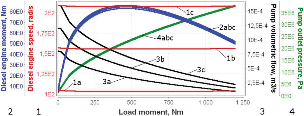
Figure 5 Dependences of the diesel engine and hydraulic pump from the actuator load moment.

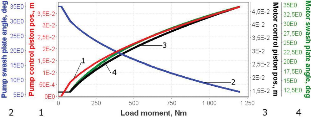
Figure 6 Dependences of automatic controls from the actuator load moment.

Figure 5 shows that angular speed of the diesel engine (graphs 1) does not depend on the actuator load moment. The moment developed by the diesel engine (graphs 2) marginally depends on the diesel engine rotating speed.

At load moments $<$ 460 Nm (graphs 2) increasing the load moment causes the diesel engine moment to rise. At load moments $>$ 460 Nm increasing the load moment causes the diesel engine moment to fall.

Volumetric flow of the hydraulic pump (graphs 3) decreases from $\sim$12e–4 m${\mathrm{}}^3$s${\mathrm{}}^{-1}$ to $\sim$1.6e–4 m${\mathrm{}}^3$s${\mathrm{}}^{-1}$ at the diesel engine rotational speed 1500 rpm. Fluid pressure at outlet of the pump (graphs 4) does not depend on the diesel engine rotating speed. The pressure increases from $\sim$1.6e6 Pa to $\sim$38e6 Pa.

In Figure 6 position of the control piston of the hydraulic pump (graph 1) changes from 0 to $\sim$0.038 m. The position angle of the hydraulic pump swash plate (graph 2) drops from 35 deg to 6 deg. The automatic control of the hydraulic pump begins at the actuator load moment $\sim$17 Nm. Position of the control piston of the hydraulic motor (graph 3) changes from $\sim$0.0145 m to $\sim$0.047 m. Position angle of the hydraulic motor swash plate (graph 4) increases from 12 deg to $\sim$34.5 deg. The automatic control of the hydraulic motor begins at the actuator load moment $\sim$75 Nm. Graphs in Figure 6 do not depend on the rotating speed of the diesel engine.

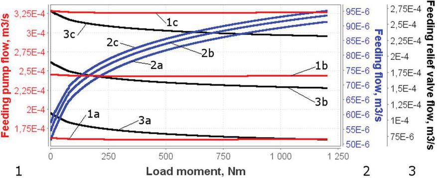
Figure 7 Dependences of the feeding volumetric flows from the actuator load moment.

In Figure 7 graphs of the feeding volumetric flows of the interface element IEH6_1-2_2 (see Figure 2) are shown. Feeding pump volumetric flow Q1 (graphs 1) and feeding volumetric flow Q2 (graphs 2) are as inputs. The feeding relief valve volumetric flow Q3 $=$ Q1 – Q2 (graphs 3) is as output. Volumetric flow of the feeding pump Q1 (graphs 1) is determined by the angular speed of the diesel engine (see Figure 5). Feeding flow Q2 (graphs 2) compensates volumetric losses and flushing flow. Initial linear part (in the load moment range 0…$\sim$75 Nm) of the graph 2 corresponds to the minimum position angle 12 deg of the hydraulic motor swash plate (see Figure 6, graph 4). Within the same load moment range volumetric flow through feeding relief valve linearly drops (graphs 3). In the load moment range $\sim$75…1200 Nm feeding volumetric flow (graphs 2) increases and feeding relief valve flow (graphs 3) drops.

Figure 8 shows that increasing the actuator load moment causes a slight decrease of feeding pressure (graphs 1) and marginal decrease of flushing pressure (graphs 2). This can be explained by the fact that at higher load moments volumetric losses and necessary feeding volumetric flow become higher (see Figure 7). Volumetric flow through pressure relief valve and feeding pressure become lower.

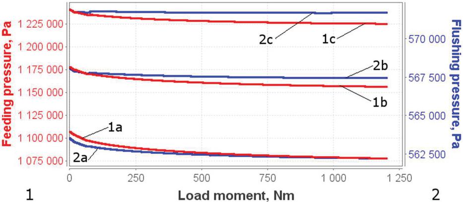
Figure 8 Dependences of the feeding and flushing pressures from the actuator load moment.

The feeding pressure is $\sim$11.6 Pa (graph 1b) and flushing pressure is $\sim$5.67e5 Pa (graph 2b) at the diesel engine rotational speed 1500 rpm and maximum load moment 1200 Nm.

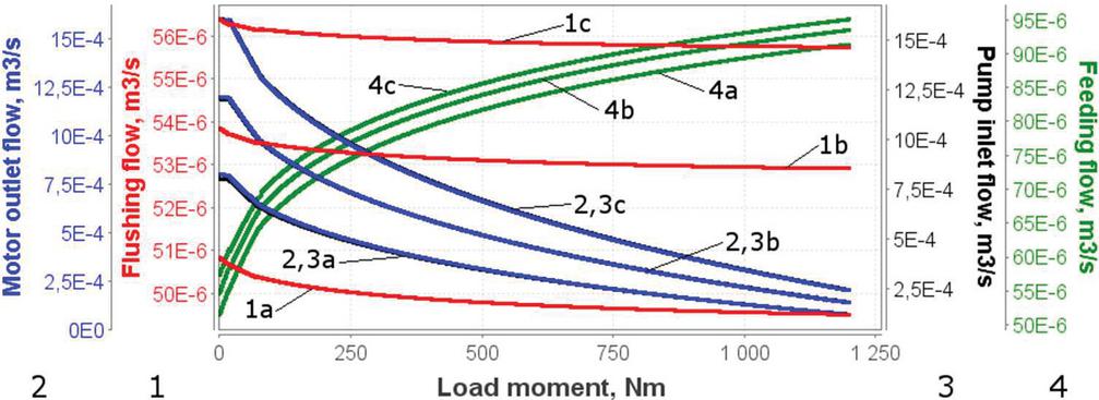
Figure 9 Dependences of hydraulic pump flows, feeding flow and flushing flow from the actuator load moment.

In Figure 9 graphs of volumetric flows of the interface element IEH6_3-1_1 (see Figure 2) are shown. Flushing volumetric flow Q1, motor outlet flow Q2 and pump inlet flow Q3 are as inputs. The feeding volumetric flow Q4 $=$ Q3 – Q2 $+$ Q1 is as an output.

At diesel engine speed 1500 rpm the hydraulic pump inlet flow Q3 (graph 3b) is $\sim$12e–4 m${\mathrm{}}^3$s${\mathrm{}}^{-1}$ at the zero load moment. The flow Q3 is $\sim$1.8e-4 m${\mathrm{}}^3$s${\mathrm{}}^{-1}$ at the maximum load moment. Hydraulic motor outlet flow Q2 (graph 2) is lower of Q3 by volumetric losses. The difference is indistinguishable from the graphs. Flushing flow Q1 (graph 1b) changes little. The average value of Q1 is $\sim$53e-6 m${\mathrm{}}^3$s${\mathrm{}}^{-1}$ at the diesel engine rotating speed n $=$ 1500 rpm. At the diesel engine rotating speed n $=$ 1500 rpm feeding volumetric flow Q4 is $\sim$55e-6 m${\mathrm{}}^3$s${\mathrm{}}^{-1}$ (graph 4b) at zero load moment and $\sim$93e-6 m${\mathrm{}}^3$s${\mathrm{}}^{-1}$ at maximum load moment 1200 Nm.

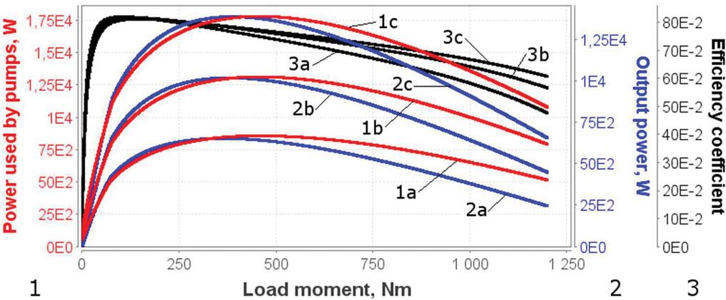
Figure 10 Dependences of powers and efficiency coefficient from the actuator load moment.

In Figure 10 values of powers used by pumps PV and PC (graphs 1), output power of the transmission (graphs 2) and efficiency coefficient of the hydraulic part of transmission (graphs 3) start from zero, reach maximum and decrease as the load moment increases. The efficiency coefficient (graph 3b) is of maximum value ${\mathrm{\eta }}_{\mathrm{m}\mathrm{a}\mathrm{x}}\approx 0.82$ at the actuator load moment 120 Nm and the diesel engine rotational speed 1500 rpm. The efficiency coefficient is $\mathrm{\eta }\approx 0.57$ at the maximum load moment 1200 Nm.

For the summer air temperature 20…30${\mathrm{}}^{\circ }$C the fluid HLP46 temperature in interval 30…40${\mathrm{}}^{\circ }$C is recommended and for winter air temperature 0…–10${\mathrm{}}^{\circ }$C the fluid HLP15 temperature in interval 10…20${\mathrm{}}^{\circ }$C. is recommended. Higher fluid temperatures cause lower efficiency coefficient, as the volumetric losses in the pump and hydraulic motor are higher.

7.3 Simulation of Dynamics

Simulation task for calculating dynamic transient responses of hydraulic closed-loop rotary transmission with automatic control of a hydraulic pump and a hydraulic motor is shown in Figure 11.

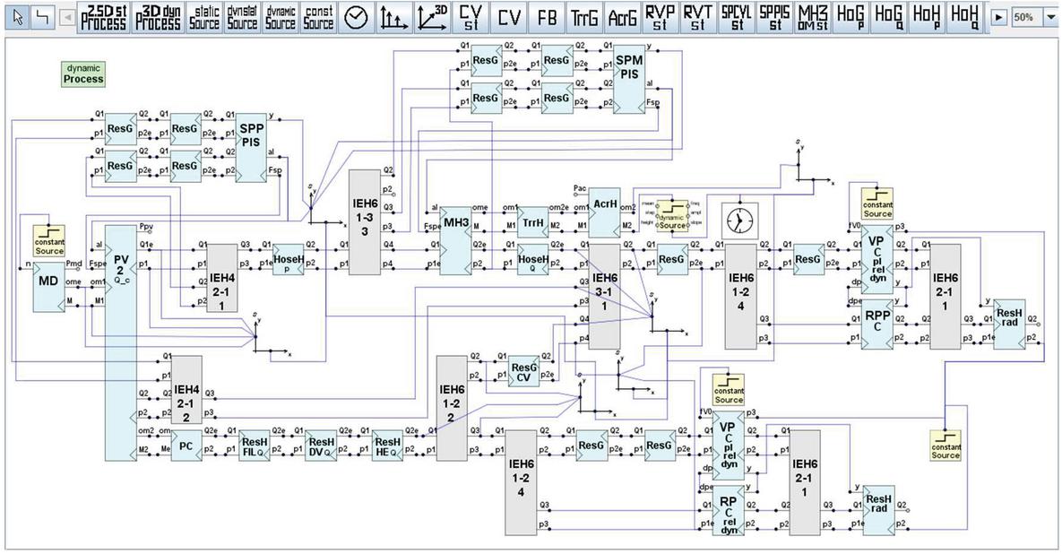
Figure 11 Dynamic simulation task of the closed-loop rotary transmission with automatic control.

The multi-pole model for dynamics differs from the model for steady state conditions (see Figure 2) in the following. A set of hydraulic resistors ResG has been added to dampen oscillations, multi-pole models of pressure relief valves elements are different (VPC_pl_rel_dyn, RPC_rel_dyn, RPPC). Hydraulic resistors ResG connected in series are used to avoid using resistors of too small diameter. In addition, the simulation task includes the following elements: process manager dynamic Process, dynamic input organiser dynamic Source and time manager Clock.

Initial values of the transmission component parameters for dynamic simulation are taken those which have been obtained as a result of simulation of steady state conditions. The simulated graphs are shown in Figures 12–17.

All the simulations of the dynamic transient responses have been performed under following conditions. Diesel engine rotational speed is taken 1500 rpm. Load moment of impulse shape is taken as an input disturbance. The mean value of the disturbance is 100 Nm, impulse height is 200 Nm, rise and drop time of the impulse is 0.01 s, duration of the impulse is 1 s. Simulation time step 1e-6 s is used, maximum simulated time is 3 s.

Figure 12 Graphs of dynamic input and output.

Graphs of the input load moment disturbance and the output angular speed of the rotary actuator are shown in Figure 12. The dynamic transient responses of the actuator output angular speed (graph 2) to impulse rise and impulse drop of the input load moment disturbance (graph 1) have exponential character. Response to impulse drop is about twice longer as the response to impulse rise.

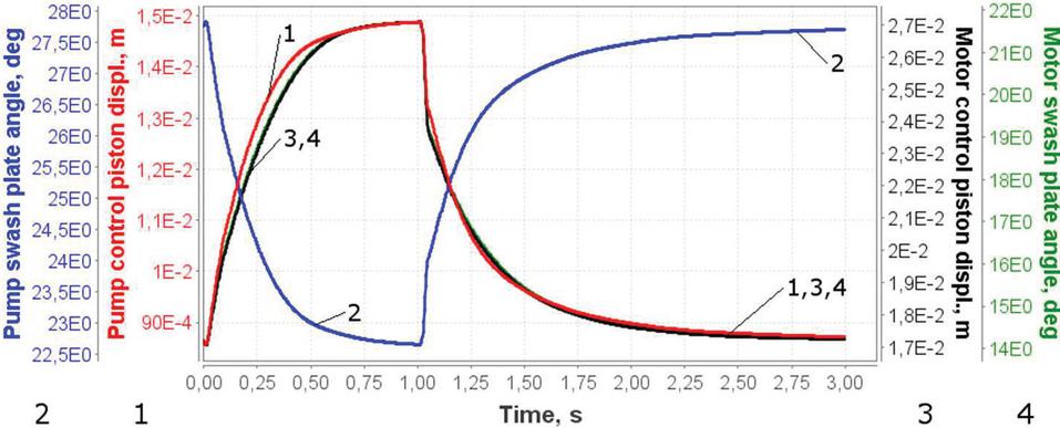
Figure 13 Graphs of hydraulic pump and motor control elements.

In Figure 13 the graphs of control pistons displacements of the hydraulic pump and motor (graphs 1, 3), and position angle of the motor swash plate (graph 4) overlap. Hydraulic pump swash plate position angle (graph 2) changes in the opposite direction.

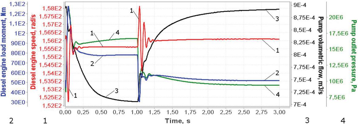
Figure 14 Graphs of diesel engine and variable displacement hydraulic pump.

In Figure 14 angular speed of the diesel engine (graph 1) oscillates at a frequency $\sim$ 15 Hz during $\sim$0.25 s as the impulse rises and falls. Transient response of the outlet volumetric flow of the hydraulic pump (graph 3) has exponential character (due to rise and drop of the input impulse) and takes more time due to the automatic control. Diesel engine load moment (graph 2) follows the behaviour of the pressure in outlet of the hydraulic pump (graph 4). All the variables shown in the graphs oscillate damped at both rise and drop of the input disturbance.

Figure 15 Graphs of volumetric flows of hydraulic pump, feeding and flushing.

In Figure 15 graphs of volumetric flows of the interface element IEH6_3-1_1 (see Figure 11) are shown. Flushing volumetric flow Q1 (graph 1), volumetric flow returned from hydraulic motor to pump Q2 (graph 2) and volumetric flow required by hydraulic pump Q3 (graph 3) are as inputs. The feeding volumetric flow Q4 (Q4 $=$ Q3 $-$ Q2 $+$ Q1) (graph 4) is as an output. Volumetric flow Q3 is higher than volumetric flow Q2. The feeding volumetric flow Q4 compensates losses in the transmission, ensures flushing and ensures normal functioning of the hydraulic pump without cavitation. All the volumetric flows oscillate damped at rise and drop of the impulse disturbance. At $\sim$1.025 s, the required feeding flow Q4 in the transient process becomes negative. To prevent this, a check valve ResG_CV is used (see Figure 17).

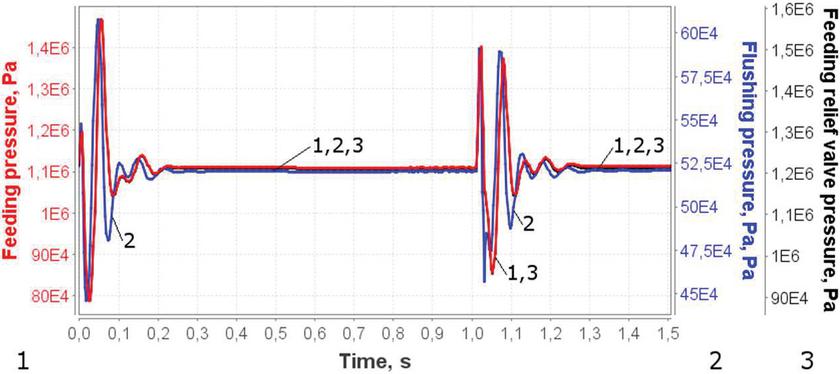
Figure 16 Graphs of feeding and flushing pressures.

In Figure 16 all the pressures oscillate damped at both rise and drop of the impulse disturbance. The oscillations take $\sim$0.25 s. Feeding pressure (graph 1) stabilizes at $\sim$11.1e5 Pa and flushing pressure (graph 2) stabilizes at $\sim$5.2e5 Pa.

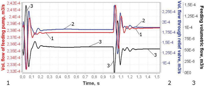
Figure 17 Graphs of feeding volumetric flows.

In Figure 17 graphs of volumetric flows of the interface element IEH6_1–2_2 (see Figure 11) are shown. Volumetric flow Q1 of feeding pump (graph 1) and feeding volumetric flow Q2 (graph 3) valve are as inputs. The volumetric flow Q3 (graph 2) through feeding pressure relief valve (Q3 $=$ Q1 $-$ Q2) is as an output. All the volumetric flows oscillate damped at both rise and drop of the impulse disturbance. The oscillations last $\sim$0.25 s. After stabilizing volumetric flow Q1 of the feeding pump is $\sim$2.38e–4 m${\mathrm{}}^3$s${\mathrm{}}^{-1}$. Volumetric flow Q2 ($\sim$1.87e–4 m${\mathrm{}}^3$s${\mathrm{}}^{-1}$) goes through feeding pressure relief valve and Q3 ($\sim$0.51e–4 m${\mathrm{}}^3$s${\mathrm{}}^{-1}$) goes for feeding the transmission.

At $\sim$1.025 s, during impulse drop (see graph 4 in Figure 15) the required feeding flow in the transient process becomes negative. To prevent feeding flow in opposite (backward) direction during the dynamic process a check valve ResG_CV is used (see Figure 11). Due to ResG_CV flow Q2 (graph 3) does not become negative.

8 Conclusions

Using computer modelling and simulation at the first stage of design of a hydraulic closed-loop rotary transmission with automatic control has been considered in the paper. Functional scheme of a closed-loop hydraulic rotary transmission with automatically controlled hydraulic pump and hydraulic motor (depending on the load moment) has been proposed. Multi-pole models of components of the transmission having various causalities are introduced and implemented for steady state conditions and dynamics. Multi-pole mathematical models of components: diesel engine, variable displacement hydraulic pump, variable displacement hydraulic motor, components of hydraulic pump and hydraulic motor control system, speed reducer, rotary actuator, etc. have been described.

Using a model-based visual simulation environment CoCoViLa (Compiler Compiler for Visual Languages) enables to describe multi-pole models graphically which facilitates the model development. The multi-pole model of the transmission is as the basis to describe the visual simulation tasks and perform simulations. Using automatic synthesis of calculation algorithms allows focusing on designing models of fluid power systems instead of constructing and solving simulation algorithms.

Implementing multi-pole models for each component gives us possibility to use distributed simulations. Calculations are performed on each component model. In case of loop dependences between component models the special iteration technique is used to solve them. Graphical simulation tasks were presented and the results of simulations were shown and discussed. As a result of the simulation a configuration of a closed-loop rotary transmission has been proposed together with constructive and operating parameters meeting the requirements.

Automatic control system proposed in the paper does not contain sensors, proportional valves, servo-valves and electronic equipment. Therefore it is of a quite simple configuration and is expected to be more reliable and cheaper.

Using the set of multi-pole models of components described in the paper and in referred papers of authors one can compose models and perform simulations for different complex fluid power systems.

Multi-pole modelling and intelligent simulation technology used in the paper can be applied in early stages of development of various technical chain systems.

Disclosure Statement

No potential conflict of interests was reported by the authors.

Funding

This research was supported by the Estonian Ministry of Research and Education institutional research grant no. IUT33-13 and The Estonian Centre of Excellence, ZEBE, grant TK146 funded by the European Regional Development Fund.

References

Aitzetmüller, H. 2000. Steyr S-matic – the future CVT system. FISITA, F2000A130.

Bosch Rexroth AG. 2005. Catalogue for the product range of hydraulic components by Bosch Rexroth, Hydraulics Industrial applications Part 1: Hydraulic pumps and motors RE 00112–01/11.05.

Cao, Q. and Zhang, M. 2010. Study on matching strategies and simulation of hydro-mechanical continuously variable transmission system of tractor. IEEE International Conference on Intelligent Computation Technology and Automation, pp. 527–530.

Grigorenko, P. et al. 2005. “COCOVILA–Compiler–Compiler for Visual Languages.” Proc. of the 5th Workshop on Language Descriptions, Tools and Applications, (Edinburgh, 2005), v. 141, n. 4 of Electron. Notes in Theor. Comput. Sci., 137–142, Elsevier.

Grigorenko, P. and Tyugu, E. 2006. “Deep Semantics of Visual Languages.” In: E. Tyugu, T. Yamaguchi (eds.) Knowledge-Based Software Engineering. Frontiers in Artificial Intelligence and Applications, vol. 140, IOS Press, 2006, 83–95.

Grossschmidt, G. and Harf, M. 2009a. “COCO–SIM–Object-oriented Multi-pole Modelling and Simulation Environment for Fluid Power Systems, Part 1: Fundamentals”. International Journal of Fluid Power, 10(2), 2009, 91–100.

Grossschmidt, G. and Harf, M. 2009b. “COCO-SIM–Object-oriented multi-pole modelling and simulation environment for fluid power systems. Part 2: Modelling and simulation of hydraulic-mechanical load-sensing system.” International Journal of Fluid Power, 10 (3), 71–85.

Grossschmidt, G. and Harf, M. 2010. “Simulation of hydraulic circuits in an intelligent programming environment, Part 1, Part 2”. 7th International DAAAM Baltic Conference “Industrial engineering”, 22–24 April 2010, Tallinn, Estonia, 148–161.

Grossschmidt, G. and Harf, M. 2012. “Multi-pole modeling and intelligent simulation of technical chain systems, Part 1, Part 2.” In: Proceedings of the 8th International Conference of DAAAM Baltic “Industrial Engineering”, Vol. 2, 19–21st April 2012, Tallinn, Estonia; (Red.) Otto, T., Tallinn; Tallinn University of Technology, 2012, 458–471.

Grossschmidt, G. and Harf, M. 2016. “Multi-pole modelling and simulation of an electro-hydraulic servo-system in an intelligent programming environment.” International Journal of Fluid Power, Vol. 17, No. 1, March 2016, Taylor & Francis, 1–13.

Grossschmidt, G. and Harf, M. 2018. “Model-based simulation of hydraulic hoses in an intelligent environment.” International Journal of Fluid Power, Vol. 19, No. 1, March 2018, Taylor & Francis, 27–41.

Harf, M. and Grossschmidt, G. 2013. “Multi-pole modelling and intelligent simulation environment for fluid power systems”. In: ESM ’2013 : The 2013 European Simulation and Modelling Conference, Modelling and Simulation, October 23–25, 2013, Lancaster University, Lancaster, UK, [Proceedings]: (Red.) Onggo, S., Kavicka, A., Ostend, Belgium: EUROSIS-ETI, 2013, 247–254.

Harf, M. and Grossschmidt, G. 2014. “Multi-pole Modeling and Intelligent Simulation of Control Valves of Fluid Power Systems. Part 1, Part 2”. In: Proceedings of the 9th International Conference of DAAAM Baltic “Industrial Engineering”; 24–26 April 2014, Tallinn, Estonia; (Red.) Otto, T., Tallinn; Tallinn University of Technology, 2014, 17–28.

Harf, M. and Grossschmidt, G. 2015. “Using Multi-pole Modelling and Intelligent Simulation in Design of a Hydraulic Drive.” In: Proceedings of the 14th International Conference on Modeling and Applied Simulation, September 21, 2015, Bergeggi, Italy, 6 p.

Kotkas, V. et al. 2011.“CoCoViLa as a multifunctional simulation platvorm.“ In: SIMUTOOLS 2011 – 4th International ICST Conference on Simulation Tools and Techniques, March 21–25, Barcelona, Spain: Brussels, ICST, 2011, 1–8.

Mollenhauer, K. and Tschöke, H. 2010. “Handbook of Diesel Engines”. Springer–Verlag, Berlin, Heidelberg, 2010.

Murrenhoff, H. 2005. “Grundlagen der Fluidtechnik, Teil 1: Hydraulik”, 4. neu überarbeitete Auflage. Institut für fluidtechnische Antriebe und Steuerungen, Aachen, 2005.

Ortwig, H. 2002. New method of numerical calculation of losses and efficiencies in hydrostatic power transmissions. SAE International Off-Highway Congress co-located with CONEXPO–CON/AGG, SAE 2002–01–1418.

Parambath, J. 2016. “Industrial Hydraulic Systems – Theory and Practice”. Universal-Publishers Boca Raton, Florida, USA, 2016.

Park, K. M. et al. 2002. The performance evaluation of servo regulator for swash plate tilting angle control of variable displacement type hydraulic piston pump. KSAE symposium, Nov, 2002, 854–859.

Qin Zhang. 2019. Basics of hydraulic systems. Second edition. 2019, by Taylor & Francis Group, LLC.

Seok Hwan Choi1 et al. 2013. Modelling and Simulation for a Tractor Equipped with Hydro-Mechanical Transmission. J. of Bio systems Eng. 38 (3): 171–179 (2013. 9).

Vacca, G. L. et al. 2007. A numerical model for the simulation of Diesel/CVT power split transmission. 8th International Conference on Engines for Automobile, SAE 2007–24–0137.

Biographies

Gunnar Grossschmidt Dipl. Eng. degree obtained from Tallinn University of Technology in 1953. Candidate of Technical Science degree (PhD) received from the Kiev Polytechnic Institute in 1959. His research interests are concentrated around modelling and simulation of fluid power systems. His list of scientific publications contains 96 items. He has been lecturing at the Tallinn University of Technology 55 years, as Assistant, Lecturer, Associate Professor, Head of the chair of Machine Design and Senior Researcher.

Mait Harf Dipl. Eng. degree obtained from Tallinn University of Technology in 1974. Candidate of Technical Science degree (PhD) received from the Institute of Cybernetics, Tallinn in 1984. His research interests are concentrated around intelligent software design. He worked on methods for automatic (structural) synthesis of programs and their applications to knowledge based programming systems such as PRIZ, C-Priz, ExpertPriz, NUT and CoCoViLa.

International Journal of Fluid Power, Vol. 21_1, 45–86.
doi: 10.13052/ijfp1439-9776.2212
© 2021 River Publishers

Abstract

1 Introduction

2 Functional Scheme of a Closed-loop Hydraulic Rotary Transmission with Automatic Control

3 Multi-pole Model of the Transmission

4 Mathematical Multi-pole Models of Components

4.1 Diesel Engine MD

4.1.1 Model of steady state conditions

4.1.2 Model of dynamics

4.1.3 Values of parameters

4.2 Variable Displacement Hydraulic Pump PV2_Q

4.2.1 Model of steady state conditions

4.2.2 Model of dynamics

4.2.3 Values of parameters

4.3 Constant Displacement Hydraulic Feeding Pump PC

4.3.1 Values of parameters

4.4 Variable Displacement Hydraulic Motor MH3

4.4.1 Values of parameters

4.5 Control Cylinders SPP_PIS and SPM_PIS

4.5.1 Model of steady state conditions

4.5.2 Model of dynamics

4.5.3 Values of parameters

4.6 Pressure Relief Valves PRV1 and PRV2

4.6.1 Poppet valve VPC_pl_rel

4.6.1.1 Model of steady state conditions

4.6.1.2 Model of dynamics

4.6.1.3 Values of parameters

4.6.2 Flow opening of poppet valve

4.6.2.1 Model of steady state conditions RPC_rel_st

4.6.2.2 Model of dynamics of feeding valve flow opening RPC_rel_dyn

4.6.2.3 Model of dynamics of flushing valve flow opening RPPC

4.6.2.4 Values of parameters

4.6.3 Spring retainer ResH_rad

4.6.3.1 Model of steady state conditions and dynamics

4.6.3.2 Values of parameters

4.7 Speed reducer TrrH

4.7.1 Model of steady state conditions

4.7.2 Model of dynamics

4.7.3 Values of parameters

4.8 Rotary Actuator AcrH

4.8.1 Model of steady state conditions

4.8.2 Model of dynamics

4.8.3 Values of parameters

4.9 Filter ResH_FIL_Q, Heater ResH_HE_Q (or Cooler ResH_CO_Q)

4.9.1 Values of parameters

4.10 Directional valve ResH_DV_Q

4.10.1 Values of parameters

4.11 Check valve ResG_CV

4.11.1 Values of parameters

4.12 Efficiency coefficient calculator EC

4.13 Hydraulic Interface Elements IEH

4.14 Other Models

5 Simulation Environment

6 Simulation Process Organization

7 Simulation

7.1 Simulation Conditions

7.2 Simulation of Steady State Conditions

7.3 Simulation of Dynamics

8 Conclusions

Disclosure Statement

Funding

References

Biographies