Fluid Stiction From a Contact Condition

Remzija Ćerimagić¹, Per Johansen^1,*, Torben Ole Andersen¹ and Rudolf Scheidl²

¹Fluid Power and Mechatronic Systems, Department of Energy Technology, Aalborg University, 9220 Aalborg East, Denmark

²Institute of Machine Design and Hydraulic Drives, Johannes Kepler University Linz, Linz, OberÖsterreich, Austria

E-mail: rec@et.aau.dk; pjo@et.aau.dk; toa@et.aau.dk; Rudolf.Scheidl@jku.at

*Corresponding Author

Received 26 October 2020; Accepted 06 May 2021; Publication 05 July 2021

Abstract

This paper considers modeling of fluid stiction between two separating plates that start from a mechanical contact condition. Published experimental work on initially contacting plates showed significant variations in stiction force peak values. In order to describe the observed strong force variations with mathematical models, the models should be quite sensitive to some of the input parameters of the stiction problem. The model in this paper assumes that small air bubbles are entrapped between the contact areas of the asperity peaks and that the fluid film flow between the cavitation bubbles is guided by Reynolds equation. The proposed model exhibits high sensitivity to initial bubble size and initial contact force compared to state-of-the art models. A delay of about 1 ms in the simulated stiction force evolution and the experiments was found. Potential causes for this discrepancy are discussed at the end of this paper and an outlook to future work, which can reduce the discrepancy between the model and experimental results is given.

Keywords: Oil stiction, fluid films, surface roughness, cavitation, Reynolds equation.

1 Introduction

Fluid stiction occurs at the lubricated interface between two bodies from the onset of a quick separation motion. It can result in very large resistive forces, hindering any immediate response to the opposing motion. This is a major drawback in fast switching valves as the fast switching capability of the valves are essential for accurate and efficient switching [1, 2]. In addition to fast switching valves, stiction effects in compressor valve technology is known to cause increased wear and noise [3, 4, 5].

In the early studies of fluid stiction Stefan [6] and later Budgett [7] conducted experimental testing and derived some general guidelines regarding the influence of different parameters on the stiction observations. It was not until the 20th century, however, that fluid stiction was treated theoretically by employing mathematical models based on theory of hydrodynamic lubrication [4, 5]. These theoretical findings showed to be in good agreement with the experimental findings of Stefan and Budgett, respectively. A series of work [1, 8, 9, 10, 11, 12] concerning oil stiction has been published in recent times. This was mainly motivated by the oil stiction problems in fast switching valves and suitable stiction models for the purpose of valve design and optimization.

The majority of the published theoretical work about fluid stiction is based on initial nonzero, fluid-filled, gaps in which the influence of surface roughness can be neglected. For example, Resch and Scheidl [10] proposed a fluid stiction model combining the Reynolds equation with cavitating zones. The pressure in the cavitation zone was assumed to be zero, hence the pressure in the surrounding fluid was alway non-negative. This stiction models showed to be in good agreement with the experimental results of Resch [9]. However, experimental results [9] with plates starting from an initial mechanical contact condition showed tensile forces of fluid film with significant variation in the stiction force peak values.

In an effort to describe fluid stiction from contact, Scheidl and Zhidong [12] proposed two different mathematical models. Both models take basis in a priori existence of cavitation nuclei in form of small bubbles. The first model was a Reynolds equation for the gap domain augmented by a Rayleigh-Plesset bubble dynamics model. However, this model exhibited a very fast dynamics of bubble growth and violated the basic condition that bubbles stay smaller than the gap. The second model is based on the hypothesis that cavitation nuclei are circular voids in the fluid film that can grow and the flow and pressure of the surrounding fluid film is guided by Reynolds equation. The model did not include surface roughness, but used an initial gap height parameter in the sense of an average value for the flow passages in the indentations of both plate surfaces. This model showed to be in reasonable agreement with the observed stiction forces from [9]. However, the model failed to capture the large variations in the observed stiction forces.

Although much work has already been dedicated to the modeling of fluid stiction, the stochastic nature of the stiction force with initially contacting plates is still troubling modern stiction models. Since initial contact of lubricated plates is a common situation suitable models for proper consideration of stiction in this case is of great practical significance. A thorough understanding of the stiction phenomenon can potentially result in the reduction of large undesirable stiction forces via optimized contact geometries.

In this work a fluid stiction from contact model in combination with a surface roughness model is proposed. The stiction model is based on the assumption that bubbles exist a priori in the fluid film and that the crevices of asperities are preferred places of the cavitation nucleus. A surface roughness model with only two peaks is taken for simplicity. The two-peak roughness model is correlated with the asperity contact model of Persson [13]. The contact model is based on Hertzian theory and should mainly reveal the effect of the fluid domain. The elastic deformation of the asperities is needed to consider the interaction of a changing boundary when the contact force is reduced and elastic contact zones shrink. Tensile stresses in the fluid domain are possible in this model. The number of bubbles, initial bubble size and the deformation of asperities are a priori unknown parameters of the model, and should be identified from experiments. The hypothesis is that the inherent stochastic nature of these parameters could explain the observed variations in the stiction forces when the contact plates are separated from an initial mechanical contact condition.

In the next section, the two-peak surface roughness model is introduced and compared with the contact model of Persson [13]. The stiction model and the numerical scheme for solving the pressure evolution in the fluid domain are subsequently described. The experimental results are described in section ’Model Evaluation with Experimental Validation’ and a comparison of the simulation model with the experiments is given. The last section describes a resume and also an outlook for how to improve the stiction model in the future.

2 Two-Peak Rough Surface Model

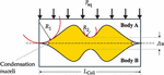
The fluid film is assumed to be enclosed between two bodies with a small annular bubble in the wedge shaped surrounding of the contact zone, see Figure 1. For simplicity, the contacting bodies (A and B) are assumed to be symmetrical and the surface roughness is represented by two asperity peaks of different height ($\mathrm{\Delta }u$) and with different radius of curvature ($R_1$ and $R_2$).

Figure 1 Schematic of the two-peak model: $p_{sq}$, squeezing pressure; $R$, radius of curvature; $\mathrm{\Delta }u$, height difference.

A mathematical model for the gap height, which allows control of the curvature radii and asperity height difference, reads

$h$	$=h_0+k_1-k_1{\mid g_1(x,y)\mid }^{n_1}\mathrm{sign}(g_1(x,y))$
	$\mathrm{\hspace{1em}}-k_2{\mid g_2(x,y)\mid }^{n_2}\mathrm{sign}(g_2(x,y))$	(1)

where

$g_1$	$={\displaystyle \frac{1}{2}}\left(1+\cos \left({\displaystyle \frac{\pi }{L_{Cell}}}(x+y)\right)\cos \left({\displaystyle \frac{\pi }{L_{Cell}}}(x-y)\right)\right)$
$g_2$	$={\displaystyle \frac{1}{2}}\left(1+\cos \left({\displaystyle \frac{\pi }{L_{Cell}}}(x+y)-\pi \right)\cos \left({\displaystyle \frac{\pi }{L_{Cell}}}(x-y)\right)\right)$

The cell length $L_{Cell}$ represents the characteristic wavelength of the two-peak model, $h_0$ is the lift-off parameter (in deformation direction) and $n_1,n_2,k_1,k_2$ are geometrical constants. The curvature at asperity peaks and height difference can be expressed in terms of the geometrical constants and cell length.

${\displaystyle \frac{1}{R_1}}$	$={\displaystyle \frac{{\pi }^2{n}_1{k}_1}{2L_{Cell}^2}}$	(2)
${\displaystyle \frac{1}{R_2}}$	$={\displaystyle \frac{{\pi }^2{n}_2{k}_2}{2L_{Cell}^2}}$	(3)
$\mathrm{\Delta }u$	$=2(k_1-k_2)$	(4)

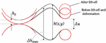
An additional measure for the roughness is the maximum height difference, i.e., the difference of maximum and minimum values of the gap height $h$ (see Equation 7). The gap geometry due the asperities and the lift-off ($h_0$) is shown in Figure 2.

$h_{max}$	$=h_0+2\left(k_1-{\displaystyle \frac{k_1}{2^{n_1}}}-{\displaystyle \frac{k_2}{2^{n_2}}}\right)$	(5)
$h_{min}$	$=h_0$	(6)
$\mathrm{\Delta }{h}_{max}$	$=2\left(k_1-{\displaystyle \frac{k_1}{2^{n_1}}}-{\displaystyle \frac{k_2}{2^{n_2}}}\right)$	(7)

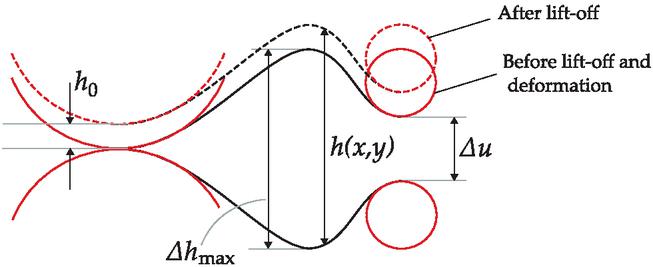
Figure 2 Gap geometry due to lift-off ($h_0$) and asperities.

2.1 Contact Geometry

It is not immediately obvious what values are appropriate for the different roughness attributes; $\mathrm{\Delta }{h}_{max},\mathrm{\Delta }u,R_1,R_2$. However, it is known from literature [14, 15, 16, 13] that rough contacting bodies show a linear relationship between contact area and load. This linear dependency comes from the random nature of the asperity shapes, in relation to the two-peak model; the statistical distribution of peak height and curvature. Thus, in order to find an appropriate contact geometry a Hertzian contact model is adopted and used to seek an optimal linearity between contact force and contact area.

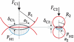
In order to find an appropriate contact geometry, contact between both asperity peaks is considered. The individual asperity peak contact is modeled as Hertzian contact of two identical spheres with the same curvature as the asperity peaks, see Figure 3.

Figure 3 Hertzian contact situation with both asperities in contact (full contact situation).

The contact circle radii and the centre deformations are given by

$a_i$	$=\sqrt[3]{{\displaystyle \frac{3F_{Ci}{R}_i}{8E^{\prime }}}}$	(8)
${\delta }_{Ci}$	$={\displaystyle \frac{2a_i^2}{R_i}}$	(9)

The reduced Young’s modulus is

$$E^{\prime }=\frac{E}{2(1-{\nu }^2)}$$

(10)

With contact forces $F_{Ci}$, Poisson’s ratio $\nu$ and Young’s modulus $E$ of the contacting bodies. The geometrical relations allows computing the centre deformations ${\delta }_{Ci}$ from the lift-off and peak height difference $h_0$ and $\mathrm{\Delta }u$, receptively.

${\delta }_{C1}$	$=-h_0$	(11)
${\delta }_{C2}$	$=-h_0-\mathrm{\Delta }u$	(12)

The total contact area is given by the sum of the contact areas at the two asperity peaks.

$$A=\pi (a_1^2+a_2^2)$$

(13)

The total contact force, i.e., the sum of the contact forces can be represented by an equivalent average contact pressure according to the formula

$$p_{sq}=\frac{F_{C1}+F_{C2}}{L_{Cell}^2}$$

(14)

The equivalent average contact pressure can be derived by solving for the Hertzian contact forces $F_{C1},F_{C2}$ in Equation (8) and substituting these into Equation (14) above. The expression for the equivalent average contact pressure in its dimensionless form is given by

$$\frac{p_{sq}}{E^{\prime }}=\sqrt{\frac{16}{18}}\left(\sqrt{R_1^{\ast }{[sg(-H_0)]}^3}+\sqrt{R_2^{\ast }{[sg(-H_0-\mathrm{\Delta }{u}^{\ast })]}^3}\right)\frac{\mathrm{\Delta }{h}_{max}}{L_{Cell}}$$

(15)

with the scales

$R_i=R_i^{\ast }{\displaystyle \frac{L_{Cell}^2}{\mathrm{\Delta }{h}_{max}}};h_0=H_0\mathrm{\Delta }{h}_{max};\mathrm{\Delta }u=\mathrm{\Delta }{u}^{\ast }\mathrm{\Delta }{h}_{max}$

(16)

The auxiliary function ‘sg’, in Equation (15), is similar to a Heaviside function and is used to smother the influence of asperities that are not in contact. Thus, for any displacement input x, the auxiliary function evaluates to:

$$sg(x)=\{\begin{array}{cc}x\hfill & \text{if }x>0\hfill \\ 0\hfill & \text{otherwise}\hfill \end{array}$$

(17)

The non-dimensional radii of curvature $R_i^{\ast }$, in Equation (15), can be expressed in terms of the exponents $n_1,n_2$ and the dimensionless height difference $\mathrm{\Delta }{u}^{\ast }$ by solving the system of equations; Equation (4) and Equation (7) for $k_1$ and $k_2$ and inserting these into Equations (2) and (3), respectively.

$R_1^{\ast }$	$={\displaystyle \frac{4(2^{n_1+n_2}-2^{n_1}-2^{n_2})}{{\pi }^2{n}_1{2}^{n_1}(2^{n_2}-\mathrm{\Delta }{u}^{\ast })}}$	(18)
$R_2^{\ast }$	$={\displaystyle \frac{4(2^{n_1+n_2}-2^{n_1}-2^{n_2})}{{\pi }^2{n}_2{2}^{n_2}(2^{n_1}-2^{n_1}\mathrm{\Delta }{u}^{\ast }+\mathrm{\Delta }{u}^{\ast })}}$	(19)

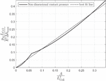
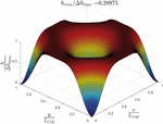
In order to validate the two-peak model a least-squares method was used to find the optimal parameter values for $n_1,n_2$. Here, the height difference $\mathrm{\Delta }{u}^{\ast }$ was chosen to be 0.5, which means that the lower peak is half the height of the larger peak. Figure 4 shows the obtained linear relationship between the dimensionless load and contact area. It indicates that the two-peak model can be brought in reasonable agreement with the theory of rough surface contact. The linearity is quite good and verifies the potential of the pseudo contact model.

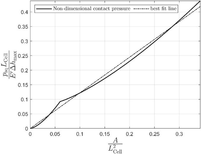
Figure 4 Dimensionless contact pressure as a function of the contact area for $\mathrm{\Delta }{u}^{\ast }=0.5$ and the optimum exponents $n_1=3.55$ and $n_2=1.45$.

2.2 Comparison with the Persson Asperity Contact Model

The two-peak model is correlated using the asperity contact model of Persson [13], which reads

$$\frac{p_{sq}}{E^{\prime }}=\beta ϵq_0{h}_{rms}\exp \left(-\frac{u\alpha }{h_{rms}}\right)$$

(20)

where

$u$ is the deformation

$p_{sq}$ is the contact pressure

$E^{\prime }$ is the reduced Young’s modulus

$h_{rms}$ is the surface root mean square roughness

$q_0$ is the roll-off wave vector of the roughness spectrum

$ϵ$ is a constant ($ϵ\approx 0.75$)

$\alpha ,\beta$ are coefficients.

The Perrson asperity contact model (Equation (20)) is selected as it has shown to be in good agreement with experimental observation [16, 17] for non-adhesive interaction and small loads. The majority of surfaces of engineering interest are self-affine fractal over a wide range of length scales with fractal dimension $d_f=2.15\pm 0.15$ [18], for which case $\alpha \approx 1$ and $\beta \approx 0.5$. The root mean square asperity height $h_{rms}$ and the wave number of roughness $q_0$ for a grinded steel surface is found in [18]. The parameters used in the Perrson model are presented in Table 1.

Table 1 Parameter set used in the model of Persson [13]

$h_{rms}$	[$\mathrm{\mu }$m]	0.5
$q_0$	[m${}^{-1}$]	1.0 $\times {10}^5$
$ϵ$	[–]	0.75
$\alpha$	[–]	1
$\beta$	[–]	0.5

For the comparison of the two-peak model with the Perrson model, the interfacial deformation is given as input. Because elastic deformation in the two-peak model occurs for $H_0=[-1;0)$, the separation motion $u$ in the Persson model corresponds to $1+H_0$ in the two-peak model. Thus, the relation between the deformation in the Persson model and the two-peak model is

$$\frac{u}{h_{rms}}=\frac{(1+H_0)\mathrm{\Delta }{h}_{max}}{h_{rms}}=\frac{1+H_0}{h_{rms,1}^{\ast }}$$

(21)

Where $h_{rms,1}^{\ast }=h_{rms}/\mathrm{\Delta }{h}_{max}$ is the nondimensional root mean square height of the two-peak model. Through numerical evaluation of the asperity heights (see Figure 5), it was found to be $h_{rms,1}^{\ast }\approx 0.29$.

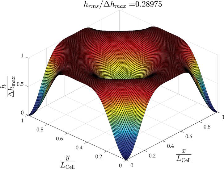
Figure 5 The total fluid gap height of the two-peak model for $n_1=3.55$, $n_2=1.45$, $\mathrm{\Delta }{u}^{\ast }=0.5$. The $h_{rms}$ value refers to the asperity height, which is the complement of the fluid gap height.

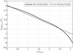
Figure 6 shows the relation between the nondimensional average contact pressure $p_{sq}/E^{\prime }$ and the interfacial deformation $u/h_{rms}$ for the two-peak model in comparison with the Persson model. It is shown that the models compare well if a proper value for $\mathrm{\Delta }{h}_{max}/L_{Cell}$ (0.04) is set. Although parameters like $h_{rms}$ of both models and $L_{Cell}$ of the two-peak model and $q_0$ of the Persson model are not directly comparable due to a big difference in the quality of the surface roughness, Figure 6 still shows a certain conformity between the models.

The range for contact area shown in Figure 4 and the elastic deformation shown in Figure 6 deem rather large, if the validity of the Herztian contact theory is considered; furthermore Persson [13] stresses the fact that elastic deformation not only comes from the Herztian contact of the asperity peaks, but also from compression of the base, which is not included in the two-peak model now. On the other hand, the two-peak model should mainly reveal the effect of the fluid domain. The elastic deformation is needed to consider the interaction of a changing boundary of the fluid domain when the elastic contact zone shrink when the contact force is reduced.

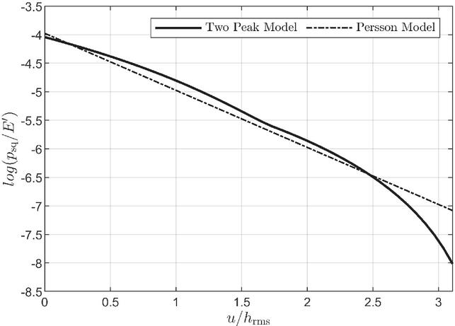
Figure 6 The dimensionless squeezing pressure $p_{sq}/E^{\prime }$ of the two-peak model and the Persson model. Two-peak model: $n_1=3.55$, $n_2=1.45$, $\mathrm{\Delta }{u}^{\ast }=0.5$, $\mathrm{\Delta }{h}_{max}/L_{Cell}=0.04$.

3 Stiction Model

In the stiction model it is assumed that the gap is made up of quadratic cells with an annular bubble in the wedge shaped surrounding of the contact zones. In this initial study of the stiction model, only the larger asperity peaks are brought into contact, see Figure 7, which is the limiting assumption of the two-peak model.

In the cell fluid domain the Reynolds equation is used to model the pressure evolution. The pressure in the bubble is assumed to decline if the bubble grows in volume following a polytropic state change model of a gas volume (Equation 22) with ambient pressure $p_{B,0}$ in the initial situation, i.e., when the bubble has initial volume $V_{B,0}$.

$$p_B=p_{B,0}{\left(\frac{V_{B,0}}{V_B}\right)}^{\kappa }$$

(22)

where

$V_B$ is the bubble volume

$p_B$ is the gas pressure inside the cavitation bubble at volume $V_B$

$\kappa$ is the polytropic exponent

$V_{B,0},p_{B,0}$ are the initial bubble volume and pressure, respectively.

It was found in [12] that the influence of surface tension is only marginal and thus not included in the current model. This means the pressure at the fluid-bubble interface ($p_F$ in Figure 7) is equal to the bubble pressure $p_B$.

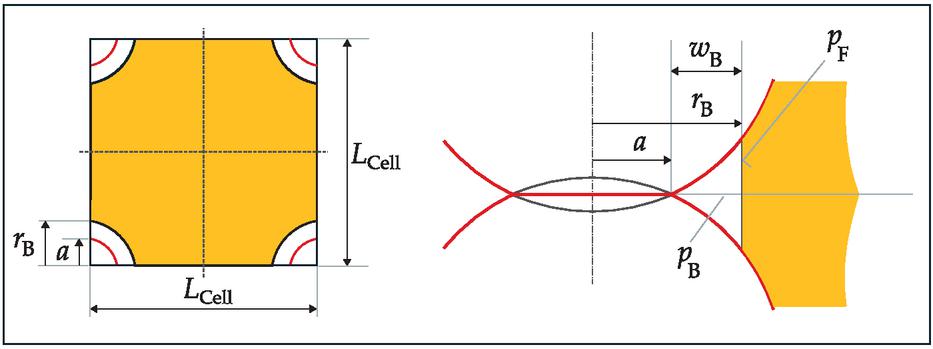
Figure 7 Geometry of the stiction model; bubbles are placed in array with pitch distance $L_{Cell}$, i.e., at the pendentives around the larger asperity peaks in contact. The origin is placed at the lower left corner of the cell on the left figure.

The formula for the bubble volume is given by Equation (23). The first term on the right-hand side of Equation (23) is related to the contact geometry and is derived under an assumption that the contact body surfaces can be approximated by the curvature of the spheres. The second term represents the void between the spherical bodies when these are released from contact (i.e., when the lift-off parameter $h_0$ is greater than zero).

$$V_B=\frac{\pi }{2R}{(r_B^2-a^2)}^2+\pi r_B^{2}sg(h_0)$$

(23)

If the liquid is assumed to be incompressible then the volume flow rate must remain the same. The flow at the bubble boundary, $Q_B$, is computed by integrating the fluid velocities along the bubble boundary.

$$Q_B={\int }_{s=0}^{s=\pi r_B/2}{v}_{\mathrm{n}}(s)h(s)ds$$

(24)

where

$s$ is a point on the bubble boundary given by the arc length

$v_{\mathrm{n}}(s)$ is fluid speed at bubble boundary point $s$

$h(s)$ is the gap height at position $s$.

The bubble volume change rate (Equation (3)) is derived by taking the derivate of the bubble volume (Equation (23)) with respect to time.

${\displaystyle \frac{\mathrm{d}{V}_B}{\mathrm{d}t}}={\displaystyle \frac{2\pi (r_B^2-a^2)(r_B{\dot{r}}_B-a\dot{a})}{R}}+2\pi r_B{\dot{r}}_{B}sg(h_0)+\pi r_B^2{\displaystyle \frac{\mathrm{d}sg(h_0)}{\mathrm{d}t}}$ (25)

The new bubble radius $r_B(t+\mathrm{\Delta }t)$ can then be computed at time $(t+\mathrm{\Delta }t)$ from the continuity relation $Q_B=\frac{\mathrm{d}{V}_B}{\mathrm{d}t}$. The new bubble radius is computed using the Euler method, i.e., $r_B(t+\mathrm{\Delta }t)=r_B(t)+\mathrm{\Delta }t{\dot{r}}_B(t)$ and making sure the continuity relation is true at any time.

4 Weighted Finite Cell Method Approach for Solving the Reynolds Equation

The experimental findings of Stefan [6] and Budgett [7] and the qualitative rules concerning the influencing problem parameters are in accordance with the classical hydrodynamic theory [10]. Thus, the Reynolds equation is used to model the pressure evolution in the fluid film. The solid bodies at the interface do not perform any in-plane motion. Then the Reynolds equation in a Cartesian coordinate system (its dimensional and non-dimensional counterpart) reads

$$\frac{\partial }{\partial x}\left(h^3\frac{\partial p}{\partial x}\right)+\frac{\partial }{\partial y}\left(h^3\frac{\partial p}{\partial y}\right)=12\mu \frac{\partial h}{\partial t}$$	(26)
$$\frac{\partial }{\partial X}\left(H^3\frac{\partial P}{\partial X}\right)+\frac{\partial }{\partial Y}\left(H^3\frac{\partial P}{\partial Y}\right)=\frac{\partial H}{\partial \tau }$$	(27)
$$p=p_{ref}P;h=\mathrm{\Delta }{h}_{max}H;x=L_{Cell}X;y=L_{Cell}Y;$$
$$t=t_{ref}\tau ;p_{ref}=\frac{12\mu L_{Cell}^2}{\mathrm{\Delta }{h}_{max}^2{t}_{ref}}$$	(28)

In this paper, a weighted finite cell method (FCM) approach is used to solve the Reynolds equation. This approach is particularly appropriate for the stiction problem as it avoids remeshing of the model at each time step due to a changing boundary of the fluid domain. In FCM the physical domain (the fluid domain) is embedded into a regular rectangular domain which is further discretized with a fixed grid of cells using higher-order B-spline basis functions [19]. An illustration of FCM for the Reynolds equation is shown in Figure 8. Due to symmetry, only a quarter of the cell is considered.

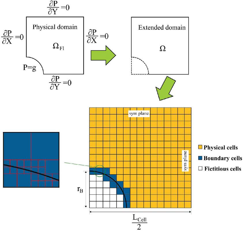
Figure 8 Schematic of the finite cell method used to solve the Reynolds equation; the original domain ${\mathrm{\Omega }}_{Fl}$ is extended to the embedding domain $\mathrm{\Omega }$, which is then subdivided into physical cells, fictitious cells and boundary cells on which a quad-tree refinement is performed.

The finite cells are divided into physical cells, fictitious cells and boundary cells according to their relative position by means of a signed distance function. Here, the signed distance function is simply given by the circle function. This approach obviates the need for an explicit formulation of the boundary; only a simple inside/outside test has to be performed for the corner points of each integration cell. Furthermore, a quad-tree refinement is applied to the boundary cells at the bubble-fluid interface in order to guarantee computing accuracy of the discretized model, see Figure 8.

Like in classical finite element method, the idea of FCM is to find the best approximation of an analytical solution by minimizing the variational functional in a finite dimensional ansatz space $V_h\subset H^1(\mathrm{\Omega })$ [20]. This is accomplished by representing the approximate solution as a linear combination of ansatz functions or shape functions that span the test space $V_h$. In this work B-splines basis functions are used as shape functions, see e.g. [21] for a definition of these basis functions.

The weak form of the nondimensional Reynolds equation with a Dirichlet boundary condition along the bubble boundary and homogeneous Neumann boundary conditions along the edges (as shown in Figure 8) can be written as $a(P,v)=l(v)$ with

$a(P,v)$	$=-{\displaystyle {\int }_{\mathrm{\Omega }}}\nabla P^T\alpha H^3\nabla v\mathrm{d}\mathrm{\Omega }$
$l(v)$	$={\displaystyle {\int }_{\mathrm{\Omega }}}{\displaystyle \frac{\partial H}{\partial \tau }}\alpha vd\mathrm{\Omega }$	(29)

Since the boundary value problem above is solved on the embedding domain, a penalty factor, $\alpha$, is here used to recover the original domain. It is defined as

$$\alpha =\{\begin{array}{cc}1\hfill & \text{if }(x,y)\in {\mathrm{\Omega }}_{Fl}\hfill \\ {10}^{-q}\hfill & \text{if }(x,y)\in \mathrm{\Omega }\backslash {\mathrm{\Omega }}_{Fl}\hfill \end{array}$$

(30)

In the fictitious domain ($\mathrm{\Omega }\backslash {\mathrm{\Omega }}_{Fl}$), the parameter $q$ should be selected as small as possible, but large enough to avoid ill-conditioning of the stiffness matrix.

Since the bubble boundary does not conform to the surface mesh, the imposition of the Dirichlet boundary condition needs special consideration. In order to impose a Dirichlet boundary condition on the bubble boundary a weighted FCM approach is taken as described in [19]. This approach is taken as it does not require additional boundary meshes. Instead of generating additional boundary meshes, a weighting function and boundary value function are used in the weighted FCM [19] to impose Dirichlet boundary conditions.

The weight function $w(x,y)$ and boundary value function $G(x,y)$ are expressed in form of implicit functions. For the nondimensional Reynolds equation these are defined as

$w$	$={\left({\displaystyle \frac{x}{L_{Cell}}}\right)}^2+{\left({\displaystyle \frac{y}{L_{Cell}}}\right)}^2-{\left({\displaystyle \frac{r_B}{L_{Cell}}}\right)}^2$	(31)
$G$	$=w+{\displaystyle \frac{p_B}{p_{ref}}}$	(32)

There are no unique expressions for the weighting function and boundary value function. However, the functions have to satisfy; $w(x,y)=0$ only on the Dirichlet boundary, and $G(x,y)=p_B$ if $w(x,y)=0$.

In this weighted interpolation scheme the numerical approximation $P_h$ is constructed as

$$P_h=\sum _{i=1}^n\sum _{j=1}^{m}w{N}_{i,j}(\xi ,\eta )q_{i,j}+G$$

(33)

with B-spline basis function $N_{i,j}$ and real coefficient $q_{i,j}\in ℝ$. By substituting the numerical approximation in Equation (29) and testing with $v=w{N}_I$ for $I=1,\mathrm{\dots },mn$, the governing system of equations $Aq=b$ reads.

$A$	$=a(w{N}_J,w{N}_I)=$
	$\mathrm{\hspace{1em}}-{\displaystyle {\int }_{\mathrm{\Omega }}}{(\nabla w{N}_J+w\nabla N_J)}^T\alpha H^3(\nabla w{N}_I+w\nabla N_I)d\mathrm{\Omega }$	(34)
$b$	$=l(w{N}_I)-a(G,w{N}_I)=$
	${\displaystyle {\int }_{\mathrm{\Omega }}}{\displaystyle \frac{\partial H}{\partial \tau }}\alpha w{N}_{I}d\mathrm{\Omega }-{\displaystyle {\int }_{\mathrm{\Omega }}}{(\nabla w{N}_I+w\nabla N_I)}^T\alpha H^3\nabla G\mathrm{d}\mathrm{\Omega }$	(35)

The Reynolds equation is solved at each time $\tau$ and for each time the weighting function and boundary value function are updated according to the current pressure $p_B(\tau )$ at bubble boundary and bubble radius $r_B(\tau )$. The total stiction force can then be computed as the sum of all the forces; from the fluid domain, the cavitation bubble and the solid body contact.

5 Model Evaluation with Experimental Validation

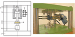
For the validation of the stiction model experimental measurements have been provided by Mrs. Eva Holl from Johannes Kepler University Linz. The experiments were carried out on a special test rig shown in Figure 9. The experiments were performed by placing an oil film on the lower plate and the plates then brought into contact by means of the servo hydraulic drive. The plates were held at a constant contact force of 20 N for 10 s followed by a fast separation motion. The experiment was repeated 10 times under the exact same conditions. The stiction force was recorded with the force sensor (6) and the gap motion by the eddy current position sensor (1), as depicted in Figure 9. The diameter of the upper plate (4) was 16.7 mm. The test fluid was a standard mineral oil based hydraulic fluid with 46 cSt nominal viscosity. It should be mentioned that the same test rig was also used in the experiments of [9] and more details on the test rig can be found in the reference.

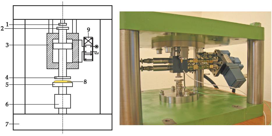
Figure 9 Fluid stiction test rig. Scheme of mechanical design and photo; components: (1): position sensor, (2): measuring object for (1), (3): hydraulic cylinder, (4,5): upper and lower stiction plate, (6): force sensor, (7): frame structure, (8): fluid film, (9): servo-valve.

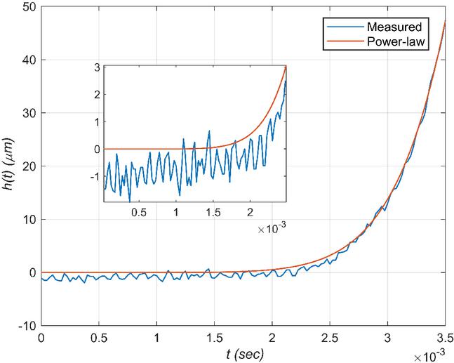
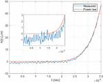
Figure 10 Input motion used in the simulation (red) and measured motion of the experiment (blue). Power-law function $h(t)=0.0021\mathrm{\mu }\mathrm{m}/{\mathrm{ms}}^8{t}^8$ identified from the the measured motion.

The main input to the stiction model is the plate separation motion. It was not possible to use the recorded plate separation motion as input in the analysis due to measurement noise in the data set. Instead the motion from the experiment was represented by a power-law model where the parameters were fitted based on the measured data. The original measured motion and the fitted regression model for the separation motion is shown in Figure 10. Further input includes the initial bubble radius $r_{B,0}$, cell length $L_{Cell}$, and the asperity heights which is dependent on the contact geometry of the two-peak model. The measured plate surface roughness values were in the ranges: $R_z:4-10\mathrm{\mu }\mathrm{m}$ $R_a:0.6-1.5\mathrm{\mu }\mathrm{m}$. These were not uniform and different in circumferential and radial direction.

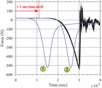
Figure 11 shows the experimental stiction force with the corresponding theoretical stiction force according to the two-peak model. In the experiments the stiction force increases first (starting from a positive stiction value due the pre-compression force) and reaches a maximum before it quickly collapses due to a reduction of flow resistance which allows fluid to fill the gap. Although, the stiction experiments were conducted under the same test conditions peak force variations of up to 20% appear in the measurements. Various attempts to reproduce the stiction results have been made by adapting the bubble size, cell length and the oil viscosity, however, it was not possible to bring the model in reasonable agreement with the measurements. There was a consistent discrepancy of approximately 1 ms between the model and the experimental results. The simulation parameters used for the computational results in Figure 11 are shown in Table 2.

An explanation why the simulated stiction force curve is faster to develop than the experimental could be unevenness of the gap profile due to manufacturing tolerances and elastic deformation. Although elastic deformations are very small they may have an influence. It makes the average gap between the plates non-uniform and the equivalent gap motion may be delayed to the position sensor signal, which shows the centre deformation of the plates and includes all other deformations of the actuation system between the position sensor and the plate contact point. Disregarding the elastic deformations may lead to an overestimation of the effective plate separation in the early phases. The release of the elastic deformation when stiction suddenly breaks down due to forming of cavitation bubbles (at approximately 3 ms in Figure 11) may also be responsible for the faster force breakdown since the effective gap opening in this phase is increased by the elastic relaxation process.

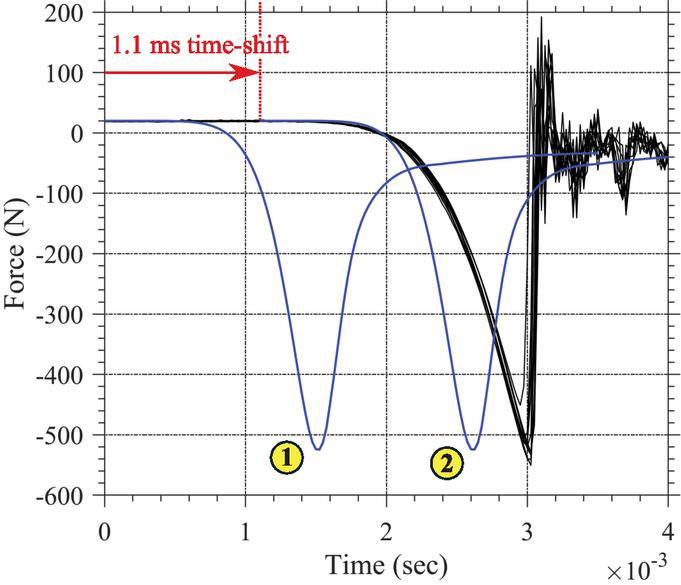
Figure 11 Comparison of the simulated stiction force (blue line) with the measured stiction force (black line).

Another major influence is the separation motion, which is the main input to the model. The approximation by a power-law may fail to represent the motion characteristics which may be composed of several phases and in which the interaction between the stiction process and the drive dynamics (the opening dynamics of servo-valve and the pressure build-up in the cylinder) is not apparent.

Table 2 Simulation parameters of the two-peak model for the results shown in Figure 11

$r_{B,0}$	[$\mathrm{\mu }$m]	60
$w_{B,0}$	[$\mathrm{\mu }$m]	7
$F_C$	[N]	20
$L_{Cell}$	[mm]	1.2
$\mu$	[Pa.s]	0.08
$E$	[GPa]	210
$\mathrm{\Delta }{h}_{max}$	[$\mathrm{\mu }$m]	48
$\mathrm{\Delta }u$	[$\mathrm{\mu }$m]	24
$R_1$	[mm]	2.3
$R_2$	[mm]	8.5

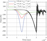
Figure 12 shows the simulated results for various initial bubble size, but otherwise same parameters as in Table 2. The actual bubble size $w_B$ is apparent from the legend in Figure 12 and it is also illustrated in Figure 7.

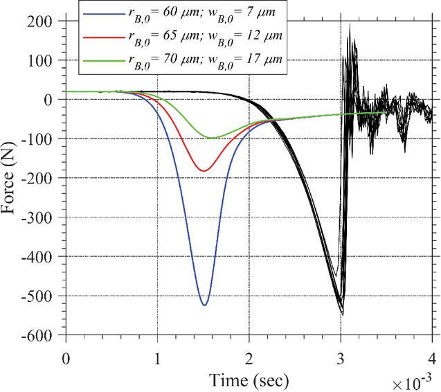
Figure 12 Simulation results for various initial bubble sizes.

The stiction force curve sensitivity to initial bubble radius is particularly interesting in the light of previous stiction force measurements [12], which showed high variations of the peak forces from experiment to experiment in some of the cases with different plate diameter and separation speed. Former attempt [12] to reproduce this force variation by variation of the initial bubble size showed that the stiction force curves were fairly unresponsive to the initial bubble size. The stiction model in this work shows to be much more responsive to variation in initial bubble size.

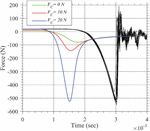
Figure 13 Simulation results for various pre-compression forces.

Figure 13 shows the stiction response for three different pre-compression forces given to the model. In each case the initial bubble radius was $r_{B,0}=60$ $\mathrm{\mu }\mathrm{m}$. The dependence of the magnitude of stiction force on the contact force is explained by the initial film thickness and the actual bubble size $w_B$ (see Figure 7). When the initial Hertz contact deformation increases when contact force $F_C$ is large the indentation increases and the initial film thickness and actual bubble size decreases. This a direct consequence of the modeling approach in which bubble is assumed entrapped between the contact areas of the asperity peaks.

6 Summary and Outlook

In this paper a fluid stiction model with surface roughness for stiction of plates starting from initial contact has been presented. The model assumes that nucleation bubbles are placed near the solid boundaries (asperities) and when the lift-off process starts the gas pressure in the these cavitation bubbles influences the fluid film flow which is governed by Reynolds equation. It was also assumed that the bubble pressure within the bubbles is uniform and depends on the bubble volume. The surface roughness profile was designed such that it was in reasonable agreement with the asperity contact model of Persson. It is shown that the model is quite sensitive to parameters like initial cavitation size and contact force, which could help explain the strong force variations observed from experimental work with initially contacting plates. However, a discrepancy in the simulated stiction forces and the experimental results of approximately 1 ms was found and the model could not be brought in agreement with the experiments. The reason for this discrepancy could be due to the elastic deformation due to compression of the base. These effects are not included in the two-peak model. The conjecture is that these deformations make the gap non-uniform, which may lead to an off-set in the effective plate displacement to the analog position sensor. Also the faster force breakdown after the stiction force reaches a maximum may be provoked by the elastic relaxation process in this phase causing a more rapid drop in flow resistance into the gap. Furthermore, sensible precaution needs to be taken when approximating the experimental motion data by a power-law as the power-law curve is no globally valid approximation and may fail to represent the essence of the interaction between the stiction process and the drive dynamics.

In order to improve the stiction model the following aspects should be considered in the future.

• The power-law motion curve is an important input to the stiction model, hence modeling of the actuation process may be necessary in order to justify the results qualitatively.

• In the two-peak model only Hertzian contact of the asperity peaks was considered mainly to reveal the effect of the fluid domain. However, a better model for the elastic deformations at the plate interface may be necessary, or at least to verify the conjecture presented in this paper.

• The simulation model is set to start from an initial contact condition, i.e. an initial contact force and initial cavitation bubble size. It might be necessary to consider the squeezing process prior to lift-off. When the average fluid gap is very small the squeezing pressure may lead to a substantial pressure build-up which may influence the initial cavitation bubble size and might also lead to a small leakage of the fluid film to the ambiance, which is not included in the current model.

• In the current model zero mass transport was assumed across the bubble/liquid interface. In further studies it might be necessary to study the influence of convective transport of the bubbles on the results.

• The current set-up most likely includes deformation of non-rigid parts including the force sensor. This could be improved by placing the displacement sensor closer to the stiction plates, see Figure 9.

Funding

This work is funded by the Danish Council for Strategic Research via the HyDrive-project (case no. 1305–00038B). The authors are grateful for the funding.

References

[1] R. Scheidl and C. Gradl. An oil stiction model for flat armature solenoid switching valves. In: Proceedings of the ASME/BATH 2013 Symposium on Fluid Power & Motion Control, October 6-9, Sarasota, Florida, USA, 2013.

[2] D. B. Roemer, P. Johansen, H. C. Pedersen, and T. O. Andersen. Fluid stiction modeling for quickly separating plates considering the liquid tensile strength. Journal of Fluids Engineering, 137(6): [061205], 2015.

[3] J. Brown, S. Pringle, A. Lough, et. al.. Oil stiction in automatic compressor valves. In Proceedings of the 14th International Congress of Refrigeration, 1975.

[4] F. Bauer. The influence of liquids on compressor valves. In Proceedings of the International Compressor Conference, 1990.

[5] H. Stehr. Oil stiction - investigations to optimize reliability of compressor valves. In Proceedings of the international conference on compressors and their systems, London, UK, September 9-12, 2001.

[6] J. Stefan. Versuche über die scheinbare Adhäsion. In: Sitzungsberichte der mathematisch-naturwissenschaftlichen Klasse der Kaiserlichen Akademie der Wissenschaften Wien, Vol. 69, Part II, pp.713-735, 1874.

[7] H. M. Budgett. The adherence of flat surfaces. Proc R Soc London Ser A, 86:25-35, 1911.

[8] M. Resch and R. Scheidl. Oil stiction in Hydraulic Valves - an Experimental Investigation. Proceedings of the ASME/BATH 2016 Symposium on Fluid Power & Motion Control, Bath, UK, 2008.

[9] M. Resch. Beiträe zum Verhalten von Newtonschen und magnetorheologischen Flüssigkeiten in engen Quetschspalten. Austrian Center of Competence in Mechatronics- Advances in Mechatronics 3. Linz: Trauner Verlag, 2011.

[10] M. Resch and R. Scheidl. A model for fluid stiction of quickly separating circular plates. Proc. of the Institution of Mechanical Engineers, Part C: Journal of Mechanical Engineering Science, 228(9): 1540-1556, 2013.

[11] R. Scheidl and C. Gradl. An approximate computational method for the fluid stiction problem of two separating parallel plates with cavitation. In: Journal of Fluids Engineering, 138(6), [061301], 2015.

[12] R. Scheidl and H. Zhidong. Fluid stiction with mechanical contact - A theoretical model. In: Proceedings of the ASME/BATH 2016 Symposium on Fluid Power & Motion Control, September 7-9, Bath, United Kingdom, 2016.

[13] B. Persson. Relation between interfacial separation and load: A general theory of contact mechanics. Phys. Rev. Lett., 99(125502), 2007.

[14] J. Archard. Elastic deformation and the laws of friction. Proc. R. Soc. A, 243:190-205, 1957.

[15] R. Onions and J. Archard. The contact of surfaces having a random structure. J. Phys. D: Appl. Phys, 6:289-304, 1973.

[16] M. Benz, K. Rosenberg, E. Kramer, and J. Israelachvili. The deformation and adhesion of randomly rough and patterned surfaces. J. Phys. Chem. B, 110:11884-11893, 2006.

[17] L. Pei, S. Hyan, J. Molinari, and M. O. Robbins. Finite element modeling of elasto-plastic contact between rough surfaces. J. Mech. Phys. Solids, 53:2385-2409, 2005.

[18] B. Persson. On the fractal dimension of rough surfaces. Tribo Lett, 54: 99-106, 2014.

[19] W. Zhang and L. Zhao. Exact imposition of inhomogeneous Dirichlet boundary conditions based on weighted finite cell method and level-set function. Comput. Methods Appl. Mech. Engrg., 307: 316-338, 2016.

[20] T. J. R. Hughes. The Finite Element Method: Linear Static and Dynamic Finite Element Analysis. Dover Publications, 1 edition, 0486411818, 2000.

[21] J. A. Cottrell, T. J. R. Hughes, and Y. Bazilevs. Isogeometric Analysis: Toward Integration of CAD and FEA. Wiley, 1 edition, 0470748737, 2009.

Biographies

Remzija Ćerimagić received his M.Sc. degree in Electro Mechanical System Design from Aalborg University, Aalborg, Denmark, in 2015. Since 2015 he has been a Ph.D. fellow at the Department of Energy Technology, Aalborg University. His research focuses on tribology modeling and simulation in fluid power pumps and motors.

Per Johansen received the B.Sc. and M.Sc. degrees in electromechanical systems engineering and the Ph.D. degree in mechanical engineering, for his studies in tribodynamic modeling, all from the Aalborg University, Aalborg, Denmark in 2009, 2011, and 2014, respectively. Since 2014, he has been at the Department of Energy Technology, Aalborg University, where he now holds the position as Associate Professor. His main research interests include Fluid power and mechatronic systems, Tribotronics, Active tribology control methods.

Torben Ole Andersen Since 2005 professor at the Department of Energy Technology, Aalborg University. Head of section: Fluid Power and Mechatronic Systems. Worked at Danfoss, R&D, as project manager and university coordinator. Research areas covers: control theory, energy usage and optimization of fluid power components and systems, mechatronic system in general, design and control of robotic systems and modelling and simulation of dynamic systems. Head of research programs relating development of a hydrostatic transmission for wind turbines and wave energy converters, and offshore mechatronic systems for autonomous operation and condition monitoring. Author and co-author of more than 250 scientific papers in international journals and conference proceedings.

Rudolf Scheidl Born November 11th 1953 in Scheibbs (Austria). MSc of Mechanical Engineering and Doctorate of Engineering Sciences at Vienna University of Technology. Industrial research and development experience in agricultural machinery (Epple Buxbaum Werke), continuous casting technology (Voest Alpine Industrieanlagenbau), and paper mills (Voith). Since Dec. 1990 Full Professor for Mechanical Engineering at the Johannes Kepler University Linz. Research topics: hydraulic drive technology and mechatronic design.

International Journal of Fluid Power, Vol. 22_3, 331–356.
doi: 10.13052/ijfp1439-9776.2232
© 2021 River Publishers

Abstract

1 Introduction

2 Two-Peak Rough Surface Model

2.1 Contact Geometry

2.2 Comparison with the Persson Asperity Contact Model

3 Stiction Model

4 Weighted Finite Cell Method Approach for Solving the Reynolds Equation

5 Model Evaluation with Experimental Validation

6 Summary and Outlook

Funding

References

Biographies