Strategies for Implementing the Jakobsson-Floberg-Olsson Cavitation Model in EHL Simulations of Translational Seals
Niklas Bauer*, Andris Rambaks, Corinna Müller, Hubertus Murrenhoff and Katharina Schmitz
RWTH Aachen University, Institute for Fluid Power Drives and Systems (ifas), Aachen, Germany
E-mail: niklas.bauer@ifas.rwth-aachen.de
*Corresponding Author
Received 30 November 2020; Accepted 19 February 2021; Publication 29 May 2021
Abstract
The numerically stable simulation of cavitation effects is mandatory for predicting the friction and wear behavior of translational hydraulic seals. This contribution provides a comparison of two different implementations of the Jakobsson-Floberg-Olsson (JFO) cavitation model, an investigation of their properties and possible options for their stabilization. These methods are tested and compared both within a simple divergent gap test case as well as within an EHL simulation of a rubber metal contact. Based on these comparisons and theoretical investigations, the strengths and weaknesses of the different methods are summarized and discussed with respect to an application in EHL simulations of translational hydraulic seals.
Keywords: Cavitation, EHL simulation, hydraulic seal, JFO model, stability.
1 Introduction
Translational hydraulic seals are widely used machine elements of crucial importance. For predicting their friction and wear behavior based on a physically motivated model, it is typically not possible to obtain an analytical solution of the equations describing the sealing contact. Therefore, numerical simulations are frequently used for this application. Besides the deformation of the seal, the friction and the distribution of the solid contact pressure, the fluid pressure distribution within the sealing gap has to be calculated. Since the flow in this application is typically laminar, the Reynolds equation can be used to describe the pressure distribution within the sealing gap. However, the solution of the Reynolds equation of incompressible fluids often provides negative pressures, contradicting with kinetic molecular theory. This, in turn, affects the calculation of the gap height and friction force, ultimately causing deviations between simulated and real behavior.
In reality, in the areas where the simulation predicts negative pressures, a gaseous phase is formed, which is known as cavitation. There are several models, which can be used to include cavitation in elastohydrodynamic lubrication (EHL) simulations. One widely used model is the Jakobsson-Floberg-Olsson (JFO) cavitation model, which has the advantageous property of mass conservation. There are several ways to implement this model in EHL simulations. However, the inclusion of such a model can cause severe instabilities. The choice of the numerical scheme for discretizing the partial derivatives directly affects the extent of these instabilities and therefore the simulation results.
This contribution compares two different approaches for the JFO model using different numerical schemes. It discusses to what extent the results differ and which model and scheme should be used for the specific application of translational hydraulic seal simulation. First, a brief overview of literature is given in Section 2. Next, Section 3 introduces the difference schemes and discusses two implementation strategies of the JFO model. The application and comparison of these methods is given both for a simple divergent gap test case in Section 4 as well as for a benchmark EHL simulation of a hydraulic seal in Section 5. Finally, the results are summarized in Section 6.
A part of the results from this contribution has already been published as a conference paper in 2020 [5].
2 Literature Review
The aim of this chapter is to give the reader an overview of the current state of research in order to understand the context. First of all, in 2.1, an overview of selected literature regarding EHL simulations in general and the simulation of elastomeric seals in particular is presented. This is followed by a description of the mathematical fundamentals in 2.2. Finally, in 2.3, the Reynolds equation and the Jakobsson-Floberg-Olsson (JFO) cavitation model are introduced.
2.1 Related Work
Several publications deal with the simulation of translational hydraulic seals. Within the finite element software Abaqus, [12] and [17] used a concept based on the User Element subroutine in order to implement the fluid pressure distribution in the sealing contact. However, these approaches do not contain a cavitation model. A similar approach was also used in [4], but was combined with the mass conserving JFO cavitation model, introduced by [10] and [11]. In [4], this model was implemented using the approach described in [20], which in turn is based on the implementation presented in [7].
An alternative approach for implementing the JFO cavitation model was introduced in [1], but, to the best of the author’s knowledge, has not been used for the simulation of dynamic seals until now. This approach does not introduce a new equation for determining the value of the cavity fraction, but uses a variable transformation instead.
2.2 Mathematical Fundamentals
Since the Reynolds equation has the form of an advection-diffusion equation, this section describes the mathematical fundamentals of such equations and possible solution methods.
Advection-diffusion of a quantity in one dimension can be modeled with the partial differential equation:
| (1) |
Equation (1) consists of a hyperbolic term, representing advection, and a parabolic term, representing diffusion. If the coefficients and are constant, an analytical solution by Fourier decomposition can be obtained for arbitrary initial profiles, where denote the Fourier coefficients [9]:
| (2) |
In practice, the coefficients are not constant and a numerical approach needs to be implemented. This presents a challenge of its own as the spatial discretization required for the advection and diffusion terms are different. Therefore, the advection equation and the diffusion equation are examined separately first.
When considering the diffusion-equation, the approximation of the second-order spatial derivative results in a central difference formula and produces a second-order accurate scheme:
| (3) |
According to [6], the scheme given by equation (3) is conditionally stable with stability criterion:
| (4) |
When considering the advection-equation, the convergence of numerical schemes depends heavily on the type of approximation used for the spatial derivative. If , a backward in space finite difference approximation must be used to guarantee conditional convergence, whereas if , a forward in space finite difference approximation must be used. This is called a first-order accurate upwind scheme, also known as the CIR scheme, and is given by:
| (5) | |||
| (6) | |||
| (7) |
According to [19], the scheme given by equation (7) is conditionally stable with a stability criterion of:
| (8) |
Disappointingly, this scheme often produces inaccurate results even for sufficiently smooth data. Hence, it is preferable to use higher-order methods, e.g. a central finite-difference approximation which is second-order accurate. However, said scheme is unconditionally unstable for non-smooth data. [19]
After examining the advection equation and diffusion equation separately, a conditionally stable scheme for the advection-diffusion equation can be formulated:
| (9) | |||
| (10) | |||
| (11) |
| (12) |
Note that the advection-diffusion equation becomes second-order accurate, i.e. reduces to the diffusion-equation if . Thus, a dimensionless quantity which describes the ratio of advection to diffusion, the Péclet number, is introduced as:
| (13) |
Equation (1) is said to be advection dominated if , and diffusion dominated if .
The Péclet number is important when a higher-order solution for the advection-diffusion equation is sought after. According to [9], it allows using unconditionally unstable central difference approximations for the spatial derivative of the advection term, if . This restriction on the Péclet number leads to oscillation-free results and overall convergence of the numerical scheme. For Péclet numbers of higher magnitude, the conditionally stable but only first-order accurate upwind schemes can be used.
In some simulations, the Péclet number varies over the computational domain. Consequently, it would be of interest to switch between higher-order methods when applicable and first-order methods when not. Fortunately, this is possible by introducing a hybrid scheme, which is given by the following equation:
| (14) |
In this numerical scheme, the spatial derivative in the advection term is approximated depending on the value of the dimensionless weighting factor , which allows switching between forward, central and backward differences by setting to , or respectively. Choosing non-integer values of can be interpreted as a convex combination of the adjacent schemes. The weighting factor can also be expressed as a function of the Péclet number, thus adapting the numerical scheme at each node according to the local advection-diffusion ratio.
2.3 The Reynolds Equation and JFO Model
In this section, both the transient Reynolds equation and the JFO cavitation model with respect to the Elrod-Adams implementation are presented.
The Reynolds equation used in this contribution includes transient effects and is extended by the flow factors introduced by [13] and the JFO cavitation model as implemented in [4] and takes the form:
| (15) |
Note, that this form of the Reynolds equation is based on the assumption that only one surface moves with the velocity . Here, denotes the fluid pressure and the gap height between the two surfaces. and are the density and dynamic viscosity of the fluid, respectively. and are the pressure and shear flow factors. denotes the root mean squared roughness.
The JFO model is included by introducing the cavity fraction , which describes the fraction of the vaporized fluid. In regions where no cavitation occurs, takes a value of zero. If the pressure drops to zero, cavitation occurs. This leads to a value of , which describes how the density of the fluid in the regions with cavitation decreases. Effectively, the density in these regions is interpolated between the liquid and the vapor. However, since the density of the vapor is small compared to the liquid, it is assumed to be zero for this contribution.
3 Implementation
The focus of this chapter is on the implementation of the EHL model used in this contribution. Section 3.1 provides an overview of the general simulation model. Two different implementations of the JFO model are presented in 3.2 and 3.3. Finally, stabilization techniques are discussed in 3.4.
3.1 Simulation Model
This section provides a brief overview of the simulation model used in this contribution. It is based on the model by [4]. For further details about the model, such as the influence of surface anisotropy and temperature, the reader is referred to [3].
The simulation model has been created using the finite element method (FEM) software Abaqus, which allows the user to extend its capabilities by adding user defined subroutines. In order to describe the sealing contact, the user subroutines User Element (UEL) and User Interaction (UINTER) are used in the simulation model. The user interaction subroutine calculates the solid contact pressure and friction, whereas the user element subroutine implements the Reynolds equation in order to calculate the fluid pressure distribution within the sealing gap.
The calculation of the solid contact is based on Persson’s contact theory [14]. It is used to calculate the normal pressure distribution based on the Young’s modulus, Poisson’s ratio and the surface topography. In contrast to other theories, this method takes into account surface roughness of all length scales. Further details about the contact model can be found e.g. in [15, 16] and [18].
The total friction force is the sum of the solid, fluid and adhesive friction forces. For further details regarding the calculation of the friction force, the reader is referred to [4].
The implementation of the fluid film is described in [2] and uses an approach similar to [12] and [17]. It is based on the Abaqus user subroutine User Element and utilizes a finite difference scheme in order to solve the Reynolds equation.
For each User Element (UEL) in Abaqus, a stiffness (Jacobian) matrix for the element and a residual vector have to be calculated. With this information available, Abaqus is able to calculate the displacement for each node of the whole model by solving the following equation:
| (16) |
In order to fully describe the behavior of the fluid at each node at the edge of the seal, four quantities must be known: the two current spatial coordinates of the nodes and , the pressure and the cavity fraction . In order to describe these quantities, the User Element used in this paper consists of two kinds of nodes.
Half the nodes are also part of the seal. The coordinates of these nodes describe the deformation of the seal at the contact and thus the gap height within the sealing gap. Therefore, the stiffness of the UEL corresponding to these nodes describes how the force exerted by the fluid on the seal changes with a varying displacement of the seal nodes.
The other half of the nodes are ghost nodes, whose coordinates do not describe a position in space, but rather the current pressure and cavity fraction at seal node . Hence, the stiffness of the UEL regarding these nodes describes how the forces on the seal change with a changing pressure respectively cavitation at node . Thus, one ghost node is necessary for each seal node affected by fluid forces, so that in order to describe the influence of the fluid on a seal edge with nodes, the UEL must consist of nodes in total.
The calculation of the displacement of the spatial nodes is based on a force equilibrium in the and direction, respectively. The displacement of the ghost nodes, which corresponds to the pressure , uses the Reynolds equation. However, since a new variable, has been introduced by the cavitation model, it is necessary to include another equation to determine the value of the new variable. As described in 2.3, if there is non-zero pressure at node i no cavitation occurs at this node:
| (17) |
Likewise, if cavitation occurs, i.e. the cavity fraction is larger than zero, the pressure has to be equal to zero:
| (18) |
And finally, both quantities and cannot be negative at any node:
| (19) |
The following Sections 3.2 and 3.3 describe two different ways to implement these relations. The first method is based on [20] and uses a Fischer-Burmeister equation for determining the value of . The second method expresses both variables and with a new variable , thus eliminating the need for an additional equation.
3.2 Using the Fischer-Burmeister Equation
Based on the work of [4] and [20], the constraint for can be implemented using a Fischer-Burmeister equation. As a first step, Equations (17) and (18) are reformulated to:
| (20) |
Combined with constraint (19), this is equivalent to considering the root of the Fischer-Burmeister function :
| (21) |
Thus, in this implementation the Reynolds equation is solved alongside equation (21). Further details about this approach are presented in [4].
3.3 Using the Combined Approach
In contrast to the previously described implementation, the method discussed in this section does not introduce a new equation, which needs to be solved, but rather a new variable . The variables and are replaced with known functions of this new variable. The approach has been presented and described in [1]. The newly introduced variable can be interpreted as a pseudo pressure, that is equal to the real pressure, if larger than zero. However, in contrast to the real pressure, can also take negative values. In that case, the magnitude of describes the amount of fluid that has vaporized. Then, the real pressure has to be equal to zero. Thus the function can be described using the piecewise linear function:
| (22) |
The function in this contribution slightly differs from the one used in [1], since it contains a hyperbolic tangent in order to prevent values of above 1.
| (23) |
Here, , , and are parameters which can be used to adjust the function. For the simulation results presented in this contribution, the set of parameters which was chosen is shown in Table 1.
Table 1 Values for the parameters of the function
3.4 Implementation of the Schemes
As can be seen in Equation (14), it is possible to define a weighting factor in order to interpolate the value of the first derivatives in a partial differential equation between the central and one-sided difference schemes. This has also been used in this contribution. Since there are two variables, for which the equation has to be solved; two weighting factors and are defined for the pressure and cavity fraction, respectively. Thus, the derivatives of and are calculated using the following expressions:
| (24) | |
| (25) |
However, in order to use these expressions, it is necessary to define values or schemes for the weighting factors. It is convenient, to use an algorithm, which calculates the values of based on the local Péclet number for the corresponding quantity. According to the schemes used in [8], which were applied to a finite volume method, five schemes are investigated in this contribution: central, upwind, exponential, hybrid and power law (PL). These schemes are defined by the following equations:
| (26) | |
| (27) | |
| (28) | |
| (29) | |
| (30) |
Figure 1 shows a plot of the weighting factor as a function of the Péclet number for the different schemes. It can be seen, that the values obtained with the exponential and the power law scheme are rather close to each other. Therefore, it can be expected, that the results obtained with these schemes do not differ considerably. Furthermore, for , the hybrid scheme generates the same values of as the central scheme. For the hybrid scheme approaches the exponential and power law schemes.
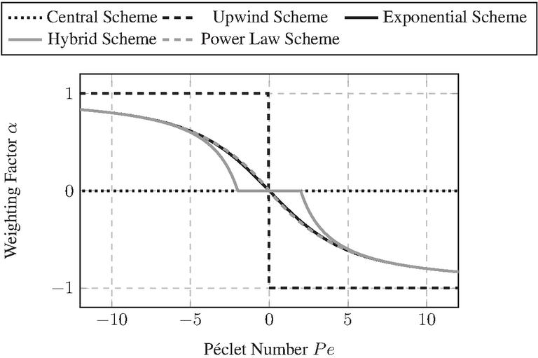
Figure 1 Plots of the weighting factor as a function of the Péclet number according to the schemes introduced in Equations (26) to (30).
Since these numerical schemes depend on the Péclet number , they can only be calculated for the Péclet number regarding the pressure , as there is no diffusive term for the cavity fraction, which leads to . Hence, only constant values are used for the weighting factor . For the calculation of , the Péclet number is derived from the Reynolds equation (15).
| (31) |
Using this notation, the advection and diffusion coefficients and can be used for calculating the Péclet number regarding the pressure :
| (32) | ||
| (33) | ||
| (34) |
4 Simulation of a Divergent Gap
In this chapter, the influence of the weighting factors and implementations introduced in Chapter 3 are compared for the simulation of the pressure distribution and cavitation within a rigid divergent gap. The parameters and setup of the test case are presented in Section 4.1. The results of this test case are given in Section 4.2 alongside a discussion in Section 4.3.
4.1 Setup of the Test Case
The simulation model consists of a rigid gap with a linearly increasing gap height as shown in Figure 2. Since the geometry is known, this test case does not require an FEM calculation. This offers two advantages: first, the two transitions from liquid phase to cavitation and vice versa can be studied isolated from deformation effects and under repeatable conditions. Secondly, the convergence behavior of the different approaches can be studied more accurately. In the full EHL simulation, no distinction between convergence behavior of the FEM and the Reynolds equation can be made. Therefore, the efficiency of the methods cannot be studied or compared accurately for a full EHL simulation, as the FEM calculation blurs the actual number of iterations required for the calculations within the gap. Since the FEM calculation of the deformation can be omitted in this test case, an accurate examination of the convergence behavior by comparing the required number of iterations is possible.
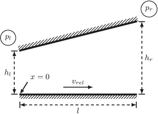
Figure 2 Divergent gap.
For this test case, the model parameters were nondimensionalized. The surfaces are assumed to be ideally smooth, so that the influence of the flow factors can be neglected (i.e. , ). The gap height is given by the linear equation . The initial pressure is given as , resulting in an initial cavitation of . The pressures at both boundaries and are both equal to . The top surface is fixed. The bottom surface is under constant acceleration , so that the relative velocity can be expressed as a function of time . The vapor pressure is set to . The full set of parameters used for the simulation is given in Table 2.
Table 2 Parameters used for the simulation of the divergent gap in Figure 2
| Number of Nodes | ||
| Simulation Time | ||
| Time Step Size | ||
| Length of the Gap | ||
| Acceleration of the Counter Surface | ||
| Density of the Fluid | ||
| Dynamic Viscosity of the Fluid | ||
| Vapor Pressure | ||
| Constant Pressure Flow Factor | ||
| Constant Shear Flow Factor | ||
| Gap Height (Left Boundary) | ||
| Gap Height (Right Boundary) | ||
| Pressure (Left Boundary) | ||
| Pressure (Right Boundary) | ||
| Initial pressure | ||
| Initial cavitation |
4.2 Results
The test case has been simulated for different values of and , both using the Fischer-Burmeister equation and the combined approach. As the purpose of this test case is to study the influence of the weighting factors themselves rather than the influence of the schemes, constant values for both weighting factors are chosen at the start of each simulation instead of a dynamical determination according to the schemes introduced in Section 3.4. The effect of the schemes will be investigated for the EHL simulation presented in Chapter 5.
The results for pressure distribution and cavity fraction at different times are shown in Figure 3. It can be seen that the pressure starts to drop with increasing time due to the increasing velocity. At , the minimum pressure is close to . At later time steps, a cavitating region in the middle of the domain is formed. Both the size of the region and the magnitude of cavitation increase during the rest of the simulation.
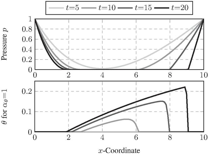
Figure 3 Pressure and cavity fraction within the gap at . All results were obtained using the implementation with the Fischer-Burmeister equation with and .
The value of either weighting factor did not show any major effect on the resulting pressure distribution. However, the cavity fraction was strongly affected by the choice of . The resulting pressure distribution and cavity fraction for different values of are shown in Figure 4. For , large oscillations can be observed. The reason for their occurrence is, that this value of the weighting factor corresponds to a central difference scheme for . Since the Reynolds equation reduces to an advection equation within cavitating regions, a central difference scheme is expected to behave unconditionally unstable. When increasing the weighting factor to , it can be seen, that the majority of the oscillations are dampened. However, close to the boundary of the cavitating region, a small peak is still visible, which disappears when choosing . In either case, there were no visible differences between the results obtained using the combined approach and the Fischer-Burmeister equation.
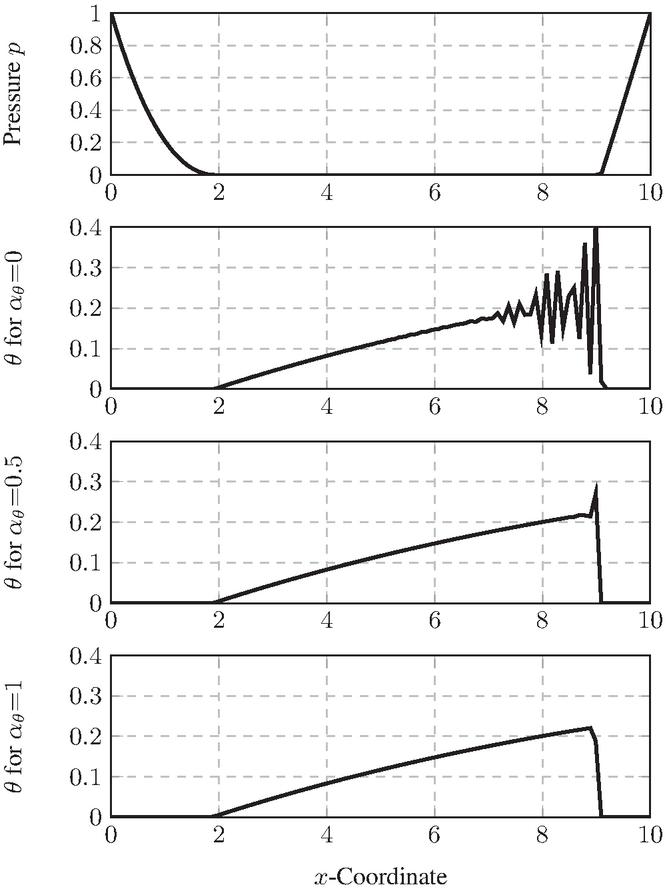
Figure 4 Pressure and cavity fraction at . Comparison of the influence of the weighting factor . All results are using the implementation with the Fischer-Burmeister equation with .
In order to investigate how the choice of the weighting factor affects the formation of the cavitating region with respect to time, the integrated cavity fraction is examined for each time step. describes the total cavity fraction at each increment and is defined as:
| (35) |
Figure 5 shows the integrated cavity fraction as a function of time for different values of . Surprisingly, even though the distribution of within the cavitating region is strongly affected by the choice of the weighting factor , see Figure 4, the integrated cavity fraction is largely unaffected by the choice of the weighting factor . Furthermore, the integrated cavity fraction is also unaffected by the choice of the implementation or .
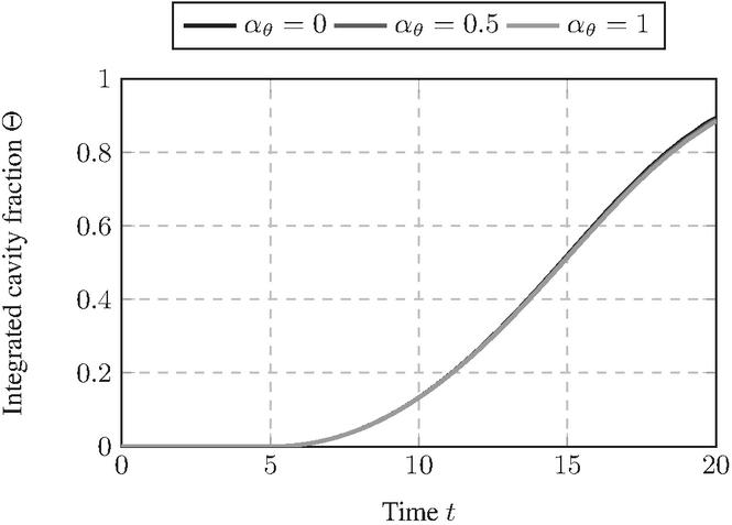
Figure 5 Integrated cavity faction for different values of . All results were obtained using the implementation with the Fischer-Burmeister equation with and .
In order to evaluate, how the convergence behavior is affected by the choice of weighting factor or implementation scheme, the number of iterations during the whole simulation is compared in Figure 6. Due to the huge instabilities for , these results are excluded from the comparison. It turns out, that the number of necessary iterations appears to be largely unaffected by the choice of the weighting factors. Neither value of the weighting factors leads to a considerable change in the number of iterations. However, choosing the combined approach reduces the number of iterations by about in comparison to the Fischer-Burmeister equation. Most likely this can be attributed to the fact, that when using the combined approach, no additional equation is introduced. The other approach introduces the Fischer-Burmeister equation, so that in this test case, each node has two degrees of freedom, the pressure and the cavity fraction , whereas in the combined approach, each node has only one degree of freedom, the auxiliary variable . Thus, the equation system which has to be solved has dimensions for the combined approach and dimensions when using the Fischer-Burmeister equation, where is the number of nodes.
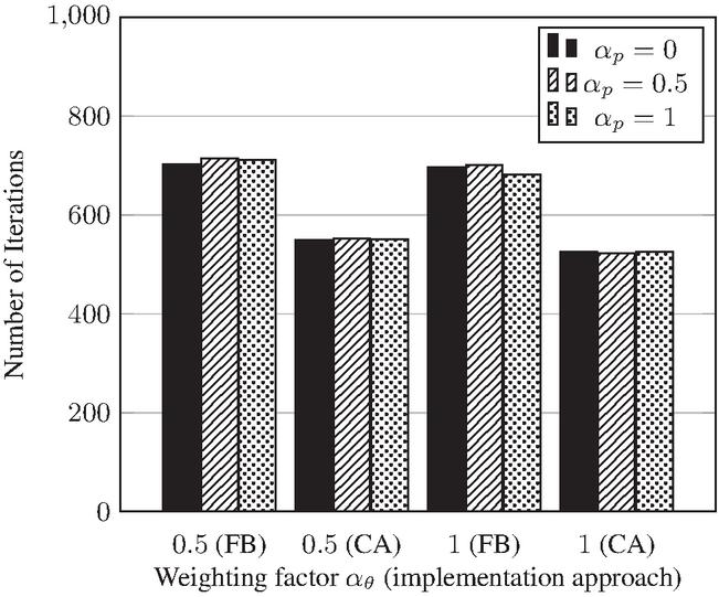
Figure 6 Total number of iterations needed for the whole simulation (200 time steps) for different values of the weighting factors , as well as for the implementations using the Fischer-Burmeister equation (FB) and the combined approach (CA).
4.3 Comparison and Discussion
In this chapter, the influence of the two weighting factors and the choice of the implementation (Fischer-Burmeister equation vs. combined approach) has been investigated for a rigid divergent gap. For studying how the cavitation is affected by the aforementioned settings, both the total amount of cavitation within the computational domain over time as well as the spatial distribution of the cavity fraction has been examined. Furthermore, the number of iterations needed for each combination of parameters and implementation has been compared.
It has been shown that within the context of the divergent gap test case, there were no noticeable differences between the different values of the weighting factor . Both the pressure distribution and the total amount of cavitation were the same regardless of the choice of it. However, the weighting factor had a strong influence on the stability of the simulation. For , large oscillations of the cavity fraction occurred. These were strongly reduced for and disappeared entirely for . The integrated cavity fraction did not show any major dependence on the choice of both weighting factors. Even in the case of the simulations with , where large instabilities of the cavitation occurred, the overall amount of cavitation within the computational domain was nearly the same as for the other simulations. The number of necessary iterations was also largely unaffected by the choice of either weighting factor. However, the simulations with the combined approach took about less iterations to complete than the simulations using the Fischer-Burmeister equation. Besides the considerable difference in the number of necessary iterations, there were no noticeable differences between the two implementations regarding the simulation results. This shows that the combined approach has the potential of reducing computational effort, especially considering that the size of the equation system, which needs to be solved, is only half as large when compared to the other approach.
5 EHL Simulation of a Hydraulic Seal
In this chapter, the results of the previously discussed implementations are presented and compared for an EHL simulation of a hydraulic seal. Here, it is of particular interest, how the choice of the cavitation model and numerical scheme affects the cavity fraction and to what extend a certain setup causes or prevents oscillations. Furthermore, the influence on the other variables of the EHL model is evaluated, by comparing the gap height, pressure distribution and friction force of the different setups. The computational efficiency of the different implementations is negligible in these considerations. It was found, that the time for calculating the solution did not differ considerably, if the solutions were converging. This can be attributed to the fact that the FEM calculation of the deformation of the seal takes considerably more time than the solution of the Reynolds equation. Thus the choice of the implementation of the cavitation model does not carry a considerable weight, when only considering the computational efficiency of the whole EHL simulation in this particular application.
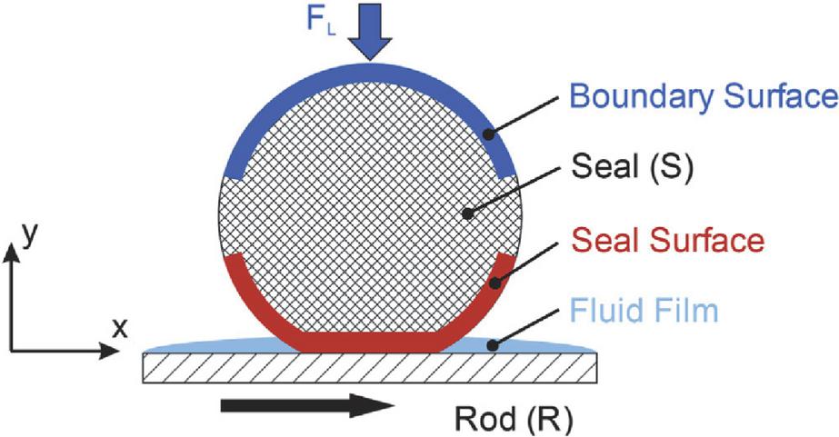
Figure 7 Schematic of the chosen test case. The movement of the nodes at the boundary surface is inhibited in -direction. The figure was taken from [4].
For comparing the performance, a two dimensional test case was selected, see Figure 7. This test case consists of an elastomeric cylinder, which represents the seal, pressed against a surface, representing the rod. After applying the force and calculating the initial deformation, the rod is accelerated with a constant acceleration . The parameters used within this chapter are shown in Table 3. Linear elastic material behavior was chosen for the rubber for the sake of simplicity. Due to the high stiffness of steel compared to rubber, the deformation of the rod was neglected entirely. Note, that since relative pressures are used for the simulation, the vapor pressure was set to corresponding to an absolute pressure of . The flow factors used in this simulation correspond to a sandblasted, thus isotropically rough, surface with a root mean squared roughness of .
Table 3 Parameters of the simulated test case
| Total Number of Nodes | ||
| Total Number of Nodes in contact | ||
| Total Number of Elements | ||
| Avg. Distance between Contact Nodes | ||
| Diameter of the Seal | ||
| Simulation Time | ||
| Acceleration of the Rod | ||
| Density of the Fluid | ||
| Dynamic Viscosity of the Fluid | ||
| Young’s Modulus Rubber | ||
| Poisson’s Ratio Rubber | ||
| Density of Rubber | ||
| Vapor Pressure | ||
| Applied Load |
The schemes introduced in 3.4 are applied for calculating the first derivative of the pressure. As it has been noted, that during the whole simulation, the hybrid scheme does not lead to results different from those obtained using the central scheme. Furthermore, as expected earlier, the results obtained using the exponential and power law scheme do not show any considerable differences. Thus, only the central, upwind and exponential scheme are used for discretizing the first derivative of the pressure for the test cases discussed in this chapter.
It has been observed, that the main stability issue of the simulation are oscillations of the cavity fraction . Therefore, the results are compared regarding the maximum value of the cavity fraction at each increment and regarding the integrated cavity fraction as defined in Equation (35).
5.1 Results Using the Fischer-Burmeister Equation
In this section, the influence of the chosen scheme and weighting factor on the results obtained using the Fischer-Burmeister equation are compared. Figure 8 shows the deformation of the seal for the different schemes at . It can be seen, that there is a steep minimum of the gap height . There are only minor deviations between the different schemes, e.g. at .
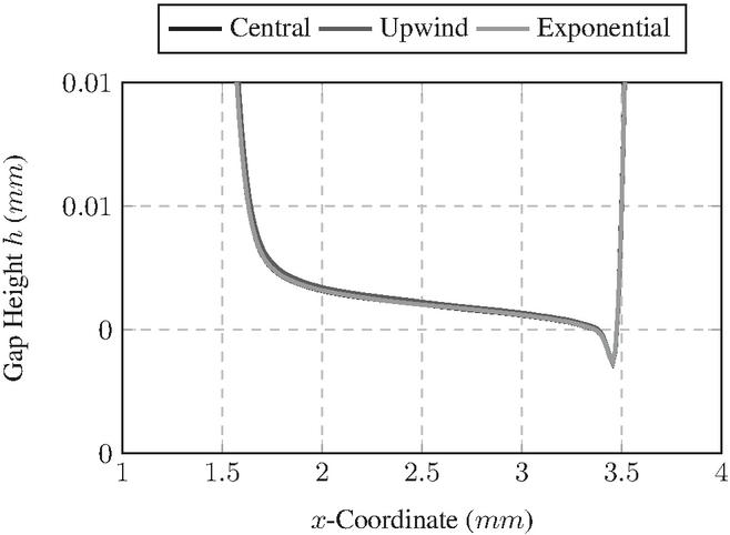
Figure 8 Comparison of the gap height at for different schemes with using the implementation with the Fischer-Burmeister equation.
The resulting pressure distribution is depicted in Figure 9. Here, it can also be seen, that there are only minor differences in the curves. A comparison of the friction force plotted against the rod velocity is presented in Figure 10. Besides minor oscillations occurring at different velocities, there are no qualitative differences in the friction behavior. These similarities were observed for all weighting factors, implementations and schemes investigated in this contribution. Thus, the focus of the investigation is on how the simulation setup affects the oscillations of the cavity fraction.
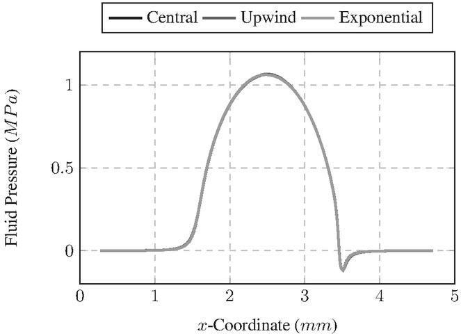
Figure 9 Comparison of the fluid pressure distribution at for different schemes with using the implementation with the Fischer-Burmeister equation.
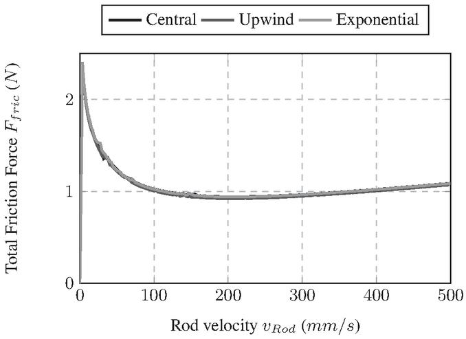
Figure 10 Comparison of the total friction force plotted against the rod velocity for different schemes with using the implementation with the Fischer-Burmeister equation.
Figure 11 shows the influence of the weighting factor on the integrated cavity fraction. For all values of , at the start of the simulation the plot is rather uneven, becoming smoother with increasing time. However, oscillations at high frequency can be observed, especially at and with . With increasing values these oscillations are considerably reduced. Also, the total value of decreases slightly.
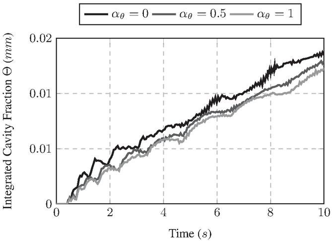
Figure 11 Comparison of the integrated cavity fraction for the central difference scheme with different as a function of time using the implementation with the Fischer-Burmeister equation.
Figure 12 shows the plot of for different weighting factors . It can be seen, that the plots show oscillations with high and low frequencies, especially for . The low frequency oscillations have a larger amplitude. This can be attributed to the fact, that the position of the maximum cavity fraction propagates with time due to the varying deformation of the seal.
It has been noticed that the cavity fraction looks similar to a Gaussian hill. Since the cavity fraction propagates slightly during the simulation, the maximum of the cavitation hill also propagates. If the maximum of the exact solution would be between two nodes, both nodes would show a rather high value of the cavity fraction. However, if the maximum of the exact solution is located exactly at the position of a single node, the value at this node would be considerably higher. Thus, even if there were no numerical deviations and with a perfect approximation to an exact solution, which looks like a Gaussian hill, the maximum of the cavity fraction would still show oscillations due to the discretization. These low frequency oscillations can be observed in all plots in this contribution. However, both the shape and the magnitude of them is affected by the choice of numerical methods.
As Figure 12 shows, the value of is significantly smaller in results obtained with higher values of . Furthermore, the amplitude of the high frequency oscillations is also reduced considerably. This behavior is typical and could be observed for all schemes and implementations investigated in this paper.
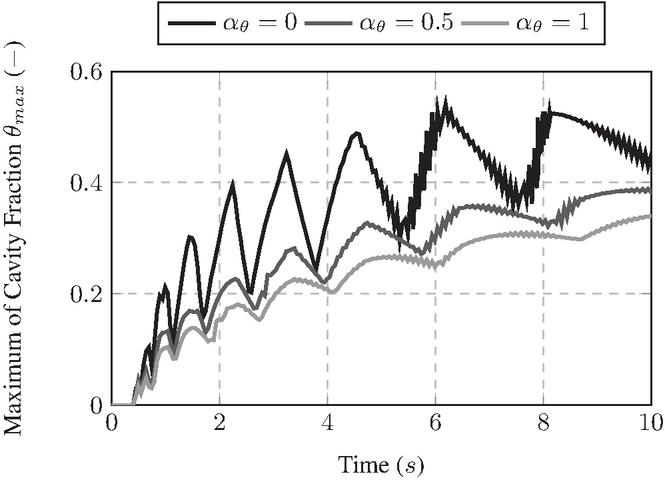
Figure 12 Comparison of the maximum value of the cavity fraction for the central difference scheme with different plotted against time using the implementation with the Fischer-Burmeister equation.
Before comparing the effects of different schemes, the distribution of the Péclet number regarding the pressure is investigated, because most of the presented schemes adjust the weighting factor for the pressure depending on the Péclet number regarding the pressure . The exemplary distribution of and the calculated are shown in Figure 13 for the exponential scheme. It can be seen, that the Péclet number takes values close to zero, except at the positions and . There, is positive and negative, respectively, with a magnitude of less than one. It can be observed, that the weighting factor adjusts accordingly, leading to an inverted shape of the curve of .

Figure 13 Distribution of the Péclet number and the weighting factor of the pressure for the exponential scheme with at using the implementation with the Fischer-Burmeister equation.
After investigating the influence of , the differences between the considered schemes are investigated. Therefore, Figures 14 and 15 show plots of and obtained using different schemes and . Here, the central and exponential scheme show a similar behavior, indicating that the weighting factors obtained are close to zero, which can also be observed in Figure 13.
Nevertheless, there are noticeable differences: first of all, both and are smaller when using the exponential scheme. Secondly, the curves obtained with the exponential scheme are slightly shifted to the left. Consequently, the results generated with the upwind differences, which use weighting factors strictly higher in magnitude than the exponential scheme, are even lower in magnitude and shifted to the left. Another difference between these curves is, that the peaks of the low frequency oscillations are smoother when using higher magnitudes of . However, regarding the high frequency oscillations of the cavity fraction, there is no visible difference between the schemes. This is reasonable, since the oscillations of the cavity fraction should not be affected by the difference scheme used for the pressure.
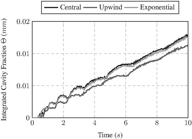
Figure 14 Comparison of the integrated cavity fraction for different schemes with as a function of time using the implementation with the Fischer-Burmeister equation.
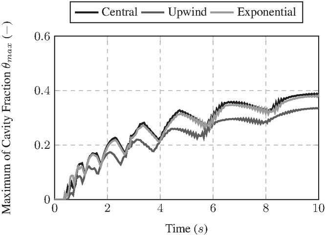
Figure 15 Comparison of the maximum value of the cavity fraction for different schemes with as a function of time using the implementation with the Fischer-Burmeister equation.
5.2 Results Using the Combined Approach
When investigating the implementation using the combined approach, it was discovered that is more prone to parameter and scheme changes than the implementation using the Fischer-Burmeister equation. Several parameter combinations did not achieve convergent results with the combined approach. For example the results obtained using the upwind scheme did not converge and are thus not shown in this section. Furthermore, for several schemes, larger values of the weighting factor were necessary in order to achieve convergent results. However, in some cases, excessive values of also did not lead to convergent results.
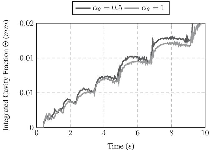
Figure 16 Comparison of the integrated cavity fraction for the central difference scheme with different as a function of time using the combined approach.
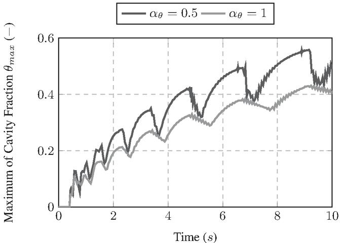
Figure 17 Comparison of the maximum value of the cavity fraction for the central difference scheme with different as a function of time using the combined approach.
Figures 16 and 17 depict the influence of different values for when using the central difference scheme. As with the implementation using the Fischer-Burmeister equation, a higher value of the weighting factor reduces the high frequency oscillations and leads to an overall smoother curve of the integrated cavity fraction .
A comparison of the different schemes is shown in Figures 18 and 19 regarding and respectively. Again there are high and low frequency oscillations visible. The amplitude of the high frequency oscillations is slightly higher when using the central scheme. As for the implementation using the Fischer-Burmeister equation, the values obtained with the exponential scheme are slightly lower and shifted to the right.

Figure 18 Comparison of the integrated cavity fraction for different schemes with as a function of time using the combined approach.
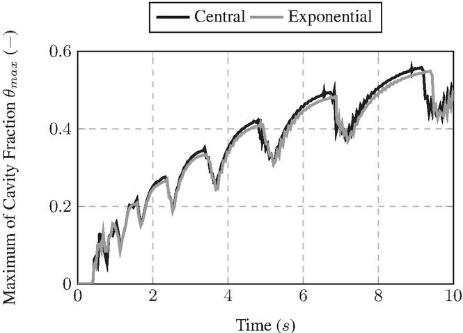
Figure 19 Comparison of the maximum value of the cavity fraction for different schemes with as a function of time using the combined approach.
5.3 Comparison and Discussion
In this section, the differences between the two investigated implementations, the Fischer-Burmeister equation on the one hand and the combined approach on the other, are shown. Figure 20 depicts the integrated cavity fraction for two different values compared for the two different approaches using the central scheme. The curves using the combined approach show higher values and more severe oscillations.
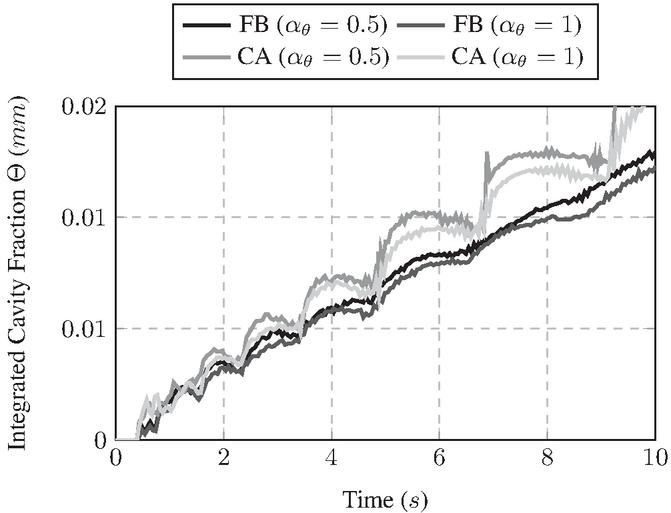
Figure 20 Comparison of the integrated cavity fraction for the central scheme with different values for and different implementations (Fischer-Burmeister (FB) and Combined Approach (CA)).
Regarding the weighting factor , it is evident that higher values of lead to a reduction of oscillations and are therefore a suitable tool for stabilizing the values of , e.g. see Figure 12. This is in line with the results of Chapter 4 and also reasonable, since in the regions with cavitation, the equation reduces to an advection equation, where upwind schemes (i.e. ) are expected to produce convergent results. However, in some simulations, such as the one using the combined approach and the exponential scheme, a value of did in fact not lead to convergent results. This can possibly be attributed to effects related to the transition from the region without cavitation to the region with cavitation.
When comparing the schemes for the first derivative of the pressure , it can be seen that the higher the magnitude of , the smoother the low frequency oscillations of the cavity fraction. Furthermore, these curves are slightly shifted to the left. However, the high frequency oscillations are largely unaffected by the choice of difference scheme. Therefore, it can be concluded, that the choice of difference scheme for the weighting factor for the cavity fraction is of higher importance than the choice of difference scheme for the pressure , which is, again, in accordance with the results of Chapter 4.
The presented implementation using the Fischer-Burmeister equation has proven to be more robust than one using the combined approach, since in the latter case, more simulations did not reach convergence. The tendency of the combined approach to cause more severe and thus potentially critical oscillations can also be observed in Figure 20. However, this implementation has the potential to decrease the computation time. This has been shown in Chapter 4 for the divergent gap test case, where the combined approach delivered the same results as the Fischer-Burmeister equation but reached convergence after fewer iterations. Yet the effect could not be observed for the full EHL simulation investigated in this chapter. Nonetheless, this potential might possibly be further explored by calculating the Péclet number not for and individually, but for itself. Using this concept, the adjustment of the difference schemes at the transition from cavitating to non-cavitating regions and vice versa might lead to more stable and smooth results for the combined approach.
6 Conclusion and Outlook
This contribution has shown the influence of different implementations and numerical schemes on the solution of the Reynolds equation with the JFO cavitation model with application to EHL simulations of translational hydraulic seals. It was shown, that the results of the gap height and pressure distribution are essentially unaffected by the choice of implementation or scheme. Therefore, the focus was on determining the influence on the oscillations of the cavity fraction. In the investigations, higher weighting factors for the cavity fraction lead to a reduction of the oscillations.
When comparing the different approaches, there were noticeable differences in stability. In this contribution, the stability of the approach with the Fischer-Burmeister equation has been less prone to parameter changes than the combined approach. When using the latter, several parameter combinations were not able to produce convergent results for the full EHL simulation. However, while investigating the divergent gap test case, the simulations using the combined approach reached convergence faster than the ones using the Fischer-Burmeister equation.
There is still potential for further investigations. On the one hand, a test of the implementations within more benchmark cases might provide additional insight into the performance of the different approaches. Both equally application-oriented and additional simple test cases could serve the purpose to understand, why the Fischer-Burmeister equation performed better in the EHL test case, whereas the combined approach converged faster during the simple test case. On the other hand, different numerical schemes, such as second and higher order schemes, and different functions for are also promising additions to the introduced approaches. In addition, considering a single Péclet number for instead of two individual ones for the pressure and the cavity fraction might lead to a further reduction of the oscillations.
Acknowledgment
The research work was performed within a Reinhart-Koselleck project funded by the German Research Foundation. We would like to thank DFG for the project support under the reference German Research Foundation DFG-Grant: MU 1225/36-1.
References
[1] Shivam Alakhramsing, Ron Ostayen, and Rob Eling. Thermo-hydrodynamic analysis of a plain journal bearing on the basis of a new mass conserving cavitation algorithm. Lubricants — Open Access Tribology Journal, 2015:256–280, 2015.
[2] Julian Angerhausen, Hubertus Murrenhoff, Leonid Dorogin, Bo Persson, and Michele Scaraggi. Influence of transient effects on the behaviour of translational hydraulic seals. In Proceedings of the 11th International Fluid Power Conference, pages 562–573, 2018.
[3] Julian Angerhausen, Hubertus Murrenhoff, Leonid Dorogin, Bo N.J. Persson, and Michele Scaraggi. The influence of temperature and surface structure on the friction of dynamic hydraulic seals. Proceedings of the 10th JFPS international Symposium on Fluid Power, pages 1C09, 1–9, 2017.
[4] Julian Angerhausen, Maik Woyciniuk, Hubertus Murrenhoff, and Katharina Schmitz. Simulation and experimental validation of translational hydraulic seal wear. Tribology International, 134:296–307, 2019.
[5] Niklas Bauer, Andris Rambaks, Hubertus Murrenhoff, and Katharina Schmitz. Implementation of the jakobsson-floberg-olsson cavitation model in an ehl simulation of translational hydraulic seals. Proceedings of the 2020 IEEE Global Fluid Power Society PhD Symposium, pages 183–193, 2020.
[6] Paul DuChateau and David W Zachmann. Applied partial differential equations. Harper & Row, 1989.
[7] H.G. ELROD and M.L. Adams. A computer program for cavitation and starvation problems. Proceedings of the 1st Leeds-Lyon Symposium on Tribology (Cavitation and Related Phenomena in Lubrication), 37, 1975.
[8] Jonathan E. Guyer, Daniel Wheeler, and James A. Warren. FiPy: Partial differential equations with Python. Computing in Science & Engineering, 11(3):6–15, 2009.
[9] Willem Hundsdorfer and Jan G Verwer. Numerical solution of time-dependent advection-diffusion-reaction equations, volume 33. Springer Science & Business Media, 2013.
[10] Bengt Jakobsson and Leif Floberg. The finite journal bearing, considering vaporization. Transactions of Chalmers University of Technology, 190, 1957.
[11] Karl-Olof Olsson. Cavitation in dynamically loaded bearings. Transactions of Chalmers University of Technology, 308:59, 1965.
[12] Yekta Öngün. Finite element simulation of mixed lubrication of highly deformable elastomeric seals. Shaker, 2010.
[13] Nadir Patir and HS Cheng. An average flow model for determining effects of three-dimensional roughness on partial hydrodynamic lubrication. Journal of Lubrication Technology, pages 12–17, 1978.
[14] B. N. J. Persson. Theory of rubber friction and contact mechanics. The Journal of Chemical Physics, 115:3840–3861, 2001.
[15] B. N. J. Persson. Relation between interfacial separation and load: A general theory of contact mechanics. Phys. Rev. Lett., 99:125502(4), 2007.
[16] M. Scaraggi and B. N. J. Persson. Friction and universal contact area law for randomly rough viscoelastic contacts. Journal of Physics: Condensed Matter, page 105102(7), 2015.
[17] T. Schmidt, M. André, and G. Poll. A transient 2d-finite-element approach for the simulation of mixed lubrication effects of reciprocating hydraulic rod seals. Tribology International, 43:1775 – 1785, 2010.
[18] A. Tiwari, L. Dorogin, M. Tahir, K. W. Stöckelhuber, G. Heinrich, N. Espallargas, and B. N. J. Persson. Rubber contact mechanics: adhesion, friction and leakage of seals. Soft Matter, pages 9103–9121, 2017.
[19] Eleuterio F Toro. Riemann solvers and numerical methods for fluid dynamics: a practical introduction. Springer Science & Business Media, 2013.
[20] Tomasz Woloszynski, Pawel Podsiadlo, and Gwidon W Stachowiak. Efficient solution to the cavitation problem in hydrodynamic lubrication. Tribology Letters, 58:18, 2015.
Biographies

Niklas Bauer studied mechanical engineering at RWTH Aachen University. Before graduating with a master’s degree in 2019, he was a student research assistant at the Chair and Institute of General Mechanics and the Chair for Computational Analysis of Technical Systems. He is a member of the scientific staff at ifas. His research interest is the numerical simulation of sealing friction.

Andris Rambaks studied mechanical engineering at Riga Technical University and later at RWTH Aachen University. In 2018, he obtained his master’s degree in mechanical engineering and is currently a member of the scientific staff at ifas. As a member of the research group fluids, his main interests are fluid properties and the numerical simulation of multiphase flow.

Corinna Müller started studying computational engineering science at RWTH Aachen University in 2018. She worked as a student research assistant at the Chair for Computational Analysis of Technical Systems. She is a student research assistant at ifas, where, her work focuses on the development and implementation of numerical methods for tribological problems.

Hubertus Murrenhoff is the former director of the Institute for Fluid Power Drives and Systems (ifas), formerly named Institute for Fluid Power Drives and Controls (IFAS) at RWTH Aachen University, Germany. Main research interests cover hydraulics and pneumatics including components, systems, controls, simulation programs and the applications of fluid power in mobile and stationary equipment.

Katharina Schmitz graduated in mechanical engineering at RWTH Aachen University in 2010 with part of her studies at Carnegie Mellon University in Pittsburgh (USA) and working in Le Havre (France). In 2015, Prof. Schmitz graduated as Dr.-Ing. Since March 2018 she is full professor at RWTH Aachen University and Director of the institute for Fluid Power Drives and Systems.
International Journal of Fluid Power, Vol. 22_2, 199–232.
doi: 10.13052/ijfp1439-9776.2223
© 2021 River Publishers