An Adaptive Robust Controller for Hydraulic Robotic Manipulators with a Flow-Mapping Compensator

Fu Zhang, Junhui Zhang^*, Bing Xu and Huizhou Zong

State Key Laboratory of Fluid Power & Mechatronic Systems, Zhejiang University, Hangzhou, 310027, China

E-mail: zhangfu@zju.edu.cn; benzjh@zju.edu.cn; bxu@zju.edu.cn; hzzong@zju.edu.cn

*Corresponding Author

Received 29 November 2020; Accepted 02 March 2021; Publication 29 May 2021

Abstract

Proportional directional control valves have flexible control functions for the control of various hydraulic manipulators. It is foreseeable that the application of proportional directional control valves will be further expanded. However, due to its own structure, its important parameter, flow gain, is complex, and it has a complex functional relationship with valve opening and temperature. The variable flow gain reduces the performance of a strictly derived nonlinear controller. Therefore, it is necessary to consider the nonlinearity of flow gain in the controller design. In order to solve the above problems, this paper proposes an adaptive robust controller for a hydraulic manipulator with a flow-mapping compensator, which takes into account the nonlinear flow gain and improves the performance of the nonlinear controller. First, we established an adaptive robust controller of the hydraulic manipulator to obtain the load flow of the control input valve. Then, the function of flow gain, input voltage, and temperature are calibrated offline using cubic polynomial, and the flow-mapping compensator is obtained. Finally, we calculate the input voltage based on the flow-mapping compensator and load flow. The flow-mapping compensator further reduces the uncertainty of the model and improves the robustness of the system. By using the proposed controller, the control accuracy of the hydraulic manipulator is significantly improved.

Keywords: Hydraulic manipulators, nonlinear control, motion control.

1 Introduction

Proportional directional control (PDC) valves are often used in casting robots, rescue robots, and underwater robots, which require a high power-to-weight ratio [1–4]. However, it is not easy to achieve high-precision control using PDC valves. The high-precision control of the hydraulic manipulator faces three challenges: the complex nonlinearity of system dynamics, the uncertainty of system parameters, and the flow gain affected by valve opening and temperature. Firstly, rigid body dynamics and pressure dynamics are highly nonlinear, and hydraulic cylinder-driven joints introduce nonlinearity. Secondly, the system has very uncertain parameters, such as load mass, friction, and oil viscosity. Thirdly, the flow gain is variable, affected by the oil temperature and valve opening. Therefore, it is incredibly challenging to achieve high-precision control of a hydraulic manipulator using PDC valves.

Nonlinear controllers have been applied to hydraulic manipulators [5–9]. These methods are based on the hydraulic manipulator model and prove the stability of the controller. These controllers take into account the nonlinearity of the system model and improve the control performance. Due to the uncertainty in the system, adaptive and adaptive robust controllers have also been proposed to improve the control performance of hydraulic manipulators. These methods can estimate uncertain parameters online. Recently, some scholars have noticed the nonlinearity of flow gain, fitting the function of valve opening and flow gain through a polynomial function [10].

In order to solve the above problems, the control accuracy of the hydraulic manipulator is further improved. We propose an adaptive robust controller with a flow-mapping compensator. According to the design steps of the adaptive robust controller, we establish an adaptive robust controller to estimate the load mass, joint friction, and oil elastic modulus online. Through the adaptive robust controller, we get the load flow. Unlike previous studies, the control current is not calculated by a nonlinear function with a fixed flow gain. We fit the function of flow gain, valve opening and temperature through a binary quartic function. A more accurate control current is calculated through the flow-mapping compensator, which improves the control accuracy of the hydraulic manipulator and the robustness of the system.

Figure 1 Multi-joint manipulator.

2 Dynamic Models

The excavator is a typical hydraulic. It is assumed that all elements in the automatic system are rigid bodies. The manipulator angle $q$ and cylinder displacement $x$ are defined, as shown in Figure 1. The arm joint of the manipulator contains two connecting links and the hydraulic cylinder, which forms a triangular closed chain, as shown in Figure 1.

The kinematic relationship between the hydraulic cylinder and the joint can be written as

${\displaystyle \frac{L_1+L_2-x^2}{2L_1{L}_2}}=\cos q$

(1)

where $L_1$ is the distance between the head-side chamber joint and the manipulator joint, $L_2$ is the distance between the rod side chamber joint and the manipulator joint, $\{\mathrm{O}\}$ is the local coordinate fixed with the manipulator.

We can convert the joint speed and hydraulic cylinder speed through a nonlinear function. The joint speed of the hydromechanical arm can be expressed as

$$\dot{q}=\frac{\partial q}{\partial x}\dot{x}=-\frac{x}{L_1{L}_2\sin q}\dot{x}$$

(2)

where $\dot{q}$ is the joint velocity, $\dot{x}$ is the cylinder velocity.

We differentiate Equation (2), we can get the expression of joint acceleration as

$$\ddot{q}=-\frac{(x\ddot{x}+{\dot{x}}^2)\sin q-x\dot{x}\dot{q}\cos q}{L_1{L}_2{(\sin q)}^2}$$

(3)

where $\ddot{q}$ is the joint acceleration, $\ddot{x}$ is the cylinder acceleration.

The actuator is an asymmetric hydraulic cylinder. There is a dual relationship between force and velocity. The dynamics of the manipulator can be written as

$$(J+m{l}^2)\ddot{q}+G(q)+mgl=\frac{\partial x}{\partial q}(P_1{A}_1-P_2{A}_2)-T$$

(4)

where $P_1$ is the pressure of the chamber without the rod, $P_2$ is the pressure of the chamber with the rod, $A_1$ is the piston area of the cylinder without the rod, $A_2$ is the piston area of the cylinder with the rod, T is the disturbance parameter including hydraulic cylinder friction torque and joint friction torque, $\mathrm{G}$ is the torque due to mechanical manipulator and load gravity, $\mathrm{J}$ is the moment of inertia relative to the coordinates $\{\mathrm{O}\}$, m is the end-load of the manipulator, and l is the distance between the end load and the coordinates $\{\mathrm{O}\}$.

When the leakage is ignored, the pressure dynamics of a hydraulic cylinder can be written as

${\displaystyle \frac{V_1}{{\beta }_e}}{\dot{P}}_1$	$=-A_1\dot{x}+Q_1=-A_1{\displaystyle \frac{\partial x}{\partial q}}\dot{q}+Q_1$	(5)
${\displaystyle \frac{V_2}{{\beta }_e}}{\dot{P}}_2$	$=A_2\dot{x}-Q_2=A_2{\displaystyle \frac{\partial x}{\partial q}}\dot{q}-Q_2$	(6)

where $V_1$ is the volume of the chamber without the rod, $V_2$ is the volume of the chamber with the rod, $Q_1$ is the supplied flow, and $Q_2$ is the return flow.

If the valve opening and the input signal of the valve port are linear, the flow equation of the servo valve can be written as

$$Q=k_{q}u\sqrt{\mathrm{\Delta }p}$$

(7)

where $k_q$ is the flow gain, $u$ is the valve input voltage, $\mathrm{\Delta }p$ is the pressure difference of the valve port.

However, the flow gain of the valve port is very complicated. It is related to the valve opening and oil temperature, and the PDC valve contains a certain area of the dead zone. These cannot be ignored. We offline tested the relationship between the valve port flow rate and the input voltage and pressure difference, as shown in Figure 2. Further, we still test the flow under oil temperature.

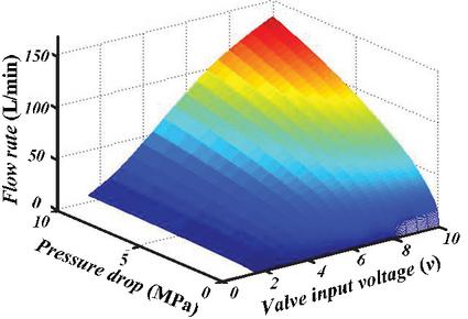
Figure 2 Multi-joint manipulator.

Therefore, achieving high precision control with the PDC valves faces not only complex dynamics in motion control of hydraulic manipulator but also the additional challenges brought by the nonlinearity of the PDC valve.

The challenges can be summarized as follows:

• It cannot be ignored that the dynamics is due to the pipeline volume and the elastic modulus of oil. The dynamics of the system contains many complex nonlinear terms.

• In the practical application process, the flow gain of a PDC valve is extremely complicated. The dead zone and nonlinear flow gain coefficient influence the dynamic characteristics and control accuracy.

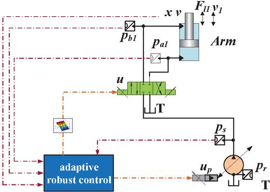
Figure 3 Presented electronic-hydraulic system.

To address these challenges, through the offline test data, we use a polynomial function to model the flow gain of the valve port and use the least square valve to fit the polynomial coefficient. We built a flow-mapping compensator and integrated it into the adaptive robust controller. The proposed controller first obtains the desired flow. Then flow-mapping compensator is used to generate an actual input signal considering the dead zone and nonlinearity of the flow model. The tiny model error is solved by particular robust feedback. By using the proposed controller, the control accuracy of the hydraulic manipulator has been significantly improved. The control frame is shown in Figure 3.

3 Controller Design

To estimate the uncertain parameters online, the uncertain parameters are further sorted, and they can be written as equations (8)–(11).

$$\theta ={[{\theta }_1{\theta }_2{\theta }_3]}^{\mathrm{T}}$$	(8)
$${\theta }_1=\frac{1}{J+ml}$$	(9)
$${\theta }_2=\frac{T+mgl}{J+ml}$$	(10)
$${\theta }_3={\beta }_{\mathrm{e}}$$	(11)

Regression form of system dynamics equation with uncertain parameters can be written as

$\ddot{q}={\theta }_1\left[{\displaystyle \frac{\partial x}{\partial q}}(P_1{A}_1-P_2{A}_2)-G(q)\right]-{\theta }_2$	(12)
${\dot{P}}_1={\displaystyle \frac{{\theta }_3}{V_1}}\left[-A_1{\displaystyle \frac{\partial x}{\partial q}}\dot{q}+Q_1+{\tilde{Q}}_1\right]$	(13)
${\dot{P}}_2={\displaystyle \frac{{\theta }_3}{V_2}}\left[A_2{\displaystyle \frac{\partial x}{\partial q}}\dot{q}-Q_2-{\tilde{Q}}_2\right]$	(14)

where ${\tilde{Q}}_1$ is supply flow error between the system model and actual system, and ${\tilde{Q}}_2$ is the return flow error between the system model and the actual system.

After the system dynamics model is established, the controller is designed according to the adaptive robust controller backstepping method.

Step 1:
There is no uncertainty in the dynamic equations of angular displacement and angular velocity, and angular velocity error $z_2$ is defined as

$$z_2={\dot{z}}_1+k_1{z}_1=\dot{q}-{\dot{q}}_r$$	(15)
$${\dot{q}}_{\mathrm{r}}\stackrel{\mathrm{\Delta }}{=}{\dot{q}}_{\mathrm{d}}-k_1{z}_1,k_1>0$$	(16)
$$z_1=q-q_d$$	(17)

where $k_1>0$, q is the actual joint angle, $q_d$ is the desired joint angle, ${\dot{q}}_r$ is the required joint angular velocity.

The positive-semidefinite Lyapunov function V${}_{\mathrm{1}}$ is defined. The function V${}_{\mathrm{1}}$ and its derivatives can be written as

$$V_1=\frac{1}{2}{w}_1{z}_1^2$$	(18)
$${\dot{V}}_1=w_1{z}_1{\dot{z}}_1=w_1{z}_1{z}_2-k_1{w}_1{z}_1^2$$	(19)

where $w_1$ is a positive constant.

If $z_2$ is as small as possible until it converges to 0, then the function ${\dot{V}}_1$, and $z_1$ converges to 0. Therefore, the next step is to design the control rate to make $z_2$ converge to 0.

Step 2:
The derivative of ${\dot{q}}_r$ is shown as Equation (20).

$${\ddot{q}}_{\mathrm{r}}={\ddot{q}}_{1\mathrm{d}}-k_1{\dot{z}}_1$$

(20)

The derivative of z${}_{\mathrm{2}}$ is shown as Equation (21).

$${\dot{z}}_2=\ddot{q}-{\ddot{q}}_{\mathrm{r}}={\theta }_1\left[\frac{\partial x}{\partial q}(P_1{A}_1-P_2{A}_2)-G(q)\right]-{\theta }_2-{\ddot{q}}_{\mathrm{r}}$$

(21)

F${}_L$ is defined as Equation (22).

$$F_{\mathrm{L}}=A_1{P}_1-A_2{P}_2$$

(22)

The virtual control input $F_{\mathrm{Lds}}$ is defined as

$$F_{\mathrm{Ld}}=F_{\mathrm{Lda}}+F_{\mathrm{Lds}}$$	(23)
$$F_{\mathrm{Lda}}={\left(\frac{\partial x}{\partial q}\right)}^{-1}\left[\frac{\ddot{q}+{\widehat{\theta }}_2-z_1}{{\widehat{\theta }}_1}-\frac{w_1{z}_1}{w_2{\widehat{\theta }}_1}+G(q)\right]$$	(24)
$$F_{\mathrm{Lds}}=F_{\mathrm{Lds1}}+F_{\mathrm{Lds2}}=-{\left(\frac{\partial x}{\partial q}\right)}^{-1}{k}_2\frac{1}{{\theta }_{1\min }}{z}_2+F_{\mathrm{Lds2}}$$	(25)

where $F_{\mathrm{Lda}}$ is synthesized to compensate nonlinear term according to the system model, using estimated parameters, ${\widehat{\theta }}_i$ is estimated parameter, $i=1,2,3,$ $F_{\mathrm{Lds1}}$ is used to stabilize the system with $k_2>0$.

The vector ${\mathit{\varphi }}_2$ and the estimated parameter error vector is defined by Equations (26)–(27).

${\varphi }_2$	$={[F_{\mathrm{Lda}},-1,0]}^T$	(26)
${\tilde{\theta }}_{\mathrm{m}}$	$={[{\tilde{\theta }}_1,{\tilde{\theta }}_2,{\tilde{\theta }}_3]}^T$	(27)

$F_{\mathrm{Lds2}}$ is used to eliminate instability caused by parameter uncertainties, which satisfy the inequalities as

$$z_2{F}_{\mathrm{Lds2}}\le 0$$	(28)
$$z_2({\mathit{\theta }}_1{F}_{\mathrm{Lds2}}-{\mathit{\varphi }}_2^T\tilde{\mathit{\theta }})\le {\epsilon }_2$$	(29)

where ${\epsilon }_2$ can measure the allowable range of error, which is a positive parameter.

Define virtual input force error z${}_{\mathrm{3}}$ as Equation (30).

$$z_3=F_{\mathrm{L}}-F_{\mathrm{Ld}}$$

(30)

The positive-semidefinite Lyapunov function $V_2$ is defined. The function $V_2$ and its derivatives can be written as

$V_2$	$=V_1+{\displaystyle \frac{1}{2}}{w}_2{z}_2^2$	(31)
${\dot{V}}_2$	$={\dot{V}}_1+w_2{z}_2{\dot{z}}_2=w_2{z}_2{\theta }_1{\displaystyle \frac{\partial x}{\partial q}}{z}_3$
	$\mathrm{\hspace{1em}}-w_2{\displaystyle \frac{{\theta }_1}{{\theta }_{1\min }}}{k}_{2s1}{z}_2^2+w_2{z}_2({\theta }_1{\mathrm{F}}_{\mathrm{Ls2}}-{\tilde{\mathit{\theta }}}^T{\mathit{\varphi }}_2)-k_1{w}_1{z}_1^2$	(32)

where $w_2$ is a positive constant.

If $z_3$ is as small as possible until it converges to 0, then the function ${\dot{V}}_2$ is less than 0, and $z_2$ converges to 0. Therefore, the next step is to design the control rate to make z${}_{\mathrm{3}}$ converge to 0.

Step 3:
The derivative of $z_3$ is shown as Equation (3).

${\dot{z}}_3$	$={\dot{F}}_{\mathrm{L}}-{\dot{F}}_{\mathrm{Ld}}=({\dot{P}}_1{A}_1-{\dot{P}}_2{A}_2)-({\dot{F}}_{\mathrm{Ldc}}+{\dot{F}}_{\mathrm{Ldu}})$
	$=-{\theta }_3\left(\left({\displaystyle \frac{A_1{}^2}{V_1}}+{\displaystyle \frac{A_2{}^2}{V_2}}\right){\displaystyle \frac{\partial x}{\partial q}}\dot{q}+{\displaystyle \frac{A_1}{V_1}}{Q}_1+{\displaystyle \frac{A_2}{V_2}}{Q}_2+{\displaystyle \frac{A_1}{V_1}}{\tilde{Q}}_1+{\displaystyle \frac{A_2}{V_2}}{\tilde{Q}}_2\right)$
	$\mathrm{\hspace{1em}}-({\dot{F}}_{\mathrm{Ldc}}+{\dot{F}}_{\mathrm{Ldu}})$	(33)

where ${\dot{F}}_{\mathrm{Ldc}}$ represents the calculable part of ${\dot{F}}_{\mathrm{Ld}}$, ${\dot{F}}_{\mathrm{Ldu}}$ is the incalculable part of ${\dot{F}}_{\mathrm{Ld}}$.

${\dot{F}}_{\mathrm{Ldc}}$ can be calculated as

$${\dot{F}}_{\mathrm{Ldc}}=\frac{\partial F_{\mathrm{Ldc}}}{\partial q}\dot{q}+\frac{\partial F_{\mathrm{Ldc}}}{\partial \dot{q}}\ddot{q}+\frac{\partial F_{\mathrm{Ldc}}}{\partial t}$$

(34)

$Q_{\mathrm{L}}$ is defined as Equation (35), and virtual control input $Q_{\mathrm{Ld}}$ as Equation (36).

$$Q_{\mathrm{L}}=\frac{A_1}{V_1}{Q}_1+\frac{A_2}{V_2}{Q}_2$$	(35)
$$Q_{\mathrm{Ld}}=Q_{\mathrm{Lda}}+Q_{\mathrm{Lds}}$$	(36)
$$Q_{\mathrm{Lda}}=\frac{1}{{\widehat{\theta }}_3}\left[{\widehat{\theta }}_3\left(\frac{A_1{}^2}{V_1}+\frac{A_2{}^2}{V_2}\right)\frac{\partial x}{\partial q}\dot{q}+{\dot{F}}_{\mathrm{Ldc}}-\frac{w_2}{w_3}{\widehat{\theta }}_1\frac{\partial x}{\partial q}{z}_2\right]$$	(37)
$$Q_{\mathrm{Lds}}=Q_{\mathrm{Lds1}}+Q_{\mathrm{Lds2}}=-k_3\frac{1}{{\theta }_{3\min }}{z}_3+Q_{\mathrm{Lds2}}$$	(38)

where $Q_{\mathrm{Lda}}$ is synthesized to compensate nonlinear term according to the system model using estimated parameters, $Q_{\mathrm{Lds1}}$ is used to stabilize the system, $k_3>0$.

The vector ${\mathit{\varphi }}_3$ is defined as Equation (39), and $Q_{\mathrm{Lds2}}$ is used to eliminate instability caused by parameter uncertainty, which satisfies the inequalities as

$${\mathit{\varphi }}_3=\left[\begin{array}{c}\hfill \frac{w_2}{w_3}{z}_2-\frac{\partial F_L}{\partial \dot{q}}(A_1{P}_1-A_2{P}_2)\hfill \\ \hfill -\frac{\partial F_L}{\partial \dot{q}}\hfill \\ \hfill -\left[\left(\frac{A_1{}^2}{V_1}+\frac{A_2{}^2}{V_2}\right)\frac{\partial x}{\partial q}\dot{q}+Q_{\mathrm{Lda}}\right]\hfill \end{array}\right]$$	(39)
$$z_3{\theta }_3{Q}_{Lds2}\le 0$$	(40)
$$z_3\left({\theta }_3{Q}_{\mathrm{Lds2}}-{\varphi }_3{}^T\tilde{\theta }+{\theta }_3\left(\frac{A_1}{V_1}{\tilde{Q}}_1+\frac{A_2}{V_2}{\tilde{Q}}_2\right)\right)\le {\epsilon }_3$$	(41)

where ${\epsilon }_3$ can measure the allowable range of error, which is a positive parameter.

The positive-semidefinite Lyapunov function $V_3$ is defined. The function $V_3$ and its derivatives can be written as

$V_3$	$=V_2+{\displaystyle \frac{1}{2}}{w}_3{z}_3^2$	(42)
${\dot{V}}_3$	$={\dot{V}}_2|{}_{z_3=0}+w_2{z}_3$
	$\mathrm{\hspace{1em}}\left(-w_3{\displaystyle \frac{{\theta }_3}{{\theta }_{3\min }}}{k}_3{z}_3^2+w_3{z}_3\left({\theta }_3\left(Q_{Lds2}+{\displaystyle \frac{A_1}{V_1}}{\tilde{Q}}_1+{\displaystyle \frac{A_2}{V_2}}{\tilde{Q}}_2\right)-{\mathit{\varphi }}_3^T\tilde{\mathit{\theta }}\right)\right)$	(43)

where $w_3$ is a positive constant.

A projection function is defined so that estimated parameters are bounded, which can be written as

$${\mathrm{Proj}}_{\theta }({\bullet }_i)=\{\begin{array}{cc}0\mathit{\hspace{1em}}\hfill & \mathrm{if}{\widehat{\theta }}_i={\theta }_{i\max }\mathrm{and}{\bullet }_i>0\hfill \\ 0\mathit{\hspace{1em}}\hfill & \mathrm{if}{\widehat{\theta }}_i={\theta }_{i\min }\mathrm{and}{\bullet }_i<0\hfill \\ {\bullet }_i\mathit{\hspace{1em}}\hfill & \mathrm{otherwise}\hfill \end{array}$$

(44)

The estimated parameter vector is updated by Equation (45)

$$\dot{\widehat{\mathit{\theta }}}={\mathrm{Proj}}_{\theta }[{\mathrm{\Gamma }}_m(w_2{\varphi }_2{z}_2+w_3{\varphi }_3{z}_3)]$$

(45)

where ${\mathbf{\Gamma }}_m$ is a positive diagonal matrix.

Through the above derivation, the control input $Q_{\mathrm{Ld}}$ is obtained.

4 Flow-Mapping Compensator and Directly Compensating Dead Zone

In this part, we introduce two methods to solve the input problem.

4.1 Flow-Mapping Compensator

To further improve the control accuracy of the hydraulic manipulator, we have established a flow-mapping compensator to calculate the input voltage according to the load flow. In this way, the problem of uncertain flow gain is solved by a flow-mapping compensator.

We test the flow of different pressure differences and different input voltages at different oil temperatures and use the least square method to fit the polynomial coefficients at this temperature. The structure of the polynomial is as Equation (46).

To calculate the valve input, a set of polynomial coefficients close to the current temperature is selected. Then the input $u$ can be solved by the equation for finding the roots of a quartic polynomial, as Equation (47).

$$c(u)=\{\begin{array}{cc}T(a{u}^3+b{u}^2+cu+d)\mathit{\hspace{1em}}\hfill & u>u_{\mathrm{de}}\hfill \\ \mathrm{\infty }\mathit{\hspace{1em}}\hfill & u_{\mathrm{de}}\le u_{\mathrm{de}}\le u_{\mathrm{de}}\hfill \\ T(-a{u}^3+b{u}^2-cu+d)\mathit{\hspace{1em}}\hfill & u<-u_{\mathrm{de}}\hfill \end{array}$$

(46)

where a, b, c and d are calculated by the least square method based on the offline measured valve pressure and flow characteristics, T is the Kelvin temperature of the oil, $u_{de}$ is the input voltage representing the dead zone.

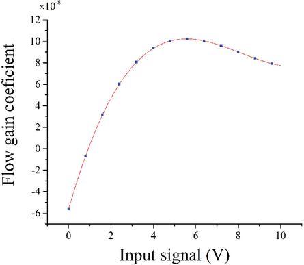
Figure 4 Presented electronic-hydraulic system.

The flow gain coefficient is fitted as a cubic curve $c(u)$, when the oil temperature in Kelvin is 313.15K, as shown in Figure 4.

$u$	$=\{\begin{array}{cc}uc(u)u={\displaystyle \frac{Q_{Ld}}{\left(\frac{A_1}{V_1}\sqrt{\mathrm{\Delta }{p}_1}+\frac{A_2}{V_2}\sqrt{\mathrm{\Delta }{p}_2}\right)}}\mathit{\hspace{1em}}\hfill & |u|>u_{\mathrm{de}}\hfill \\ 0\mathit{\hspace{1em}}\hfill & \left|u\right|\le u_{\mathrm{de}}\hfill \end{array}$	(47)
$\mathrm{\Delta }{p}_1$	$=\{\begin{array}{c}\hfill P_s-P_1{Q}_{Ld}>0\hfill \\ \hfill P_2-P_r{Q}_{Ld}<0\hfill \end{array}$	(48)
$\mathrm{\Delta }{p}_2$	$=\{\begin{array}{c}\hfill P_s-P_2{Q}_{Ld}<0\hfill \\ \hfill P_2-P_r{Q}_{Ld}>0\hfill \end{array}$	(49)

4.2 Directly Compensating Dead Zone

It is assumed that the flow gain $k_q$ is constant, and the dead zone is directly compensated, and the compensation equation can be written as Equation (50).

$$u=\frac{Q_{Ld}}{k_q(\frac{A_1}{V_1}\sqrt{\mathrm{\Delta }{p}_1}+\frac{A_2}{V_2}\sqrt{\mathrm{\Delta }{p}_2})}+u_{\mathrm{de}}sign(Q_{Ld})$$

(50)

5 Simulation Results

In this paper, the simulation models of the mechanical part and hydraulic part are established in Simcenter AMESim, and the controller is built-in Simulink. The two software co simulate through the SimulinkCosim interface.

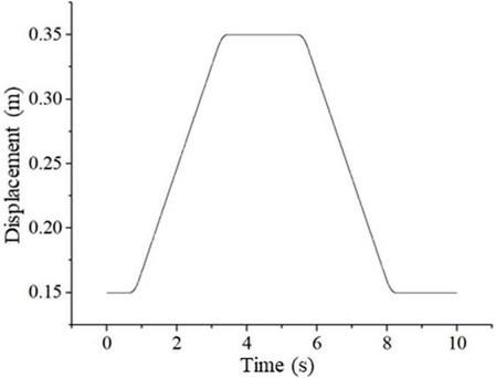
Figure 5 Tracking trajectory of hydraulic cylinder.

A trajectory is used for a comparative experiment, as shown in Figure 5, which has a maximum velocity of v= 0.08 m/s and a maximum acceleration of a $=$ 0.3 m/s${}^2$.

In the simulation experiment, the coefficients of the feedback term are $k1=15$, $k2=20$, $k3=40$, $u_{de}=1$. The adaptation update rate is written as Equation (51).

$$\mathbf{\Gamma }=\left[\begin{array}{ccc}\hfill 2\times {10}^{-8}\mathit{\hspace{1em}}\hfill & \hfill 0\mathit{\hspace{1em}}\hfill & \hfill 0\hfill \\ \hfill 0\mathit{\hspace{1em}}\hfill & \hfill 6\times {10}^{-8}\mathit{\hspace{1em}}\hfill & \hfill 0\hfill \\ \hfill 0\mathit{\hspace{1em}}\hfill & \hfill 0\mathit{\hspace{1em}}\hfill & \hfill 3\times {10}^{-6}\hfill \end{array}\right]$$

(51)

The simulation results are shown in Figure 6. With the same control parameters, the transient error of the adaptive robust controller using flow-mapping compensator is smaller, and the steady-state error of the adaptive robust controller using flow-mapping compensator can faster convergence.

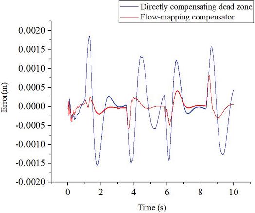
Figure 6 Tracking error of hydraulic cylinder.

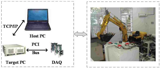
Figure 7 Presented electronic-hydraulic system.

6 Experimental Results

The controller is evaluated on the experimental platform of the hydraulic manipulator in this paper. To facilitate empirical research, the xPC Target real-time workshop is used in the control system of the hydraulic manipulator. The test platform and control system structure are shown in Figure 7. The arm joint was used as the research object for comparative experiments.

The test bench parameters required in the experiment are shown in Table 1.

Table 1 Parameters of the test rig

Parameters	Value	Unit
The maximum displacement of the pump	45.6	cm${}^3$/r
The rotational speed of the motor	1500	r/min
The diameter of the arm cylinder	0.07	m
Piston diameter of the arm cylinder	0.04	m

Two controllers are tested for comparison. They have the same control parameters. The feedback gains used are $k1=30$, $k2=25$, $k3=30$, where $u_{de}=1$. The adaptation update rate is written as Equation (52)

$$\mathbf{\Gamma }=\left[\begin{array}{ccc}\hfill 1\times {10}^{-8}\mathit{\hspace{1em}}\hfill & \hfill 0\mathit{\hspace{1em}}\hfill & \hfill 0\hfill \\ \hfill 0\mathit{\hspace{1em}}\hfill & \hfill 8\times {10}^{-8}\mathit{\hspace{1em}}\hfill & \hfill 0\hfill \\ \hfill 0\mathit{\hspace{1em}}\hfill & \hfill 0\mathit{\hspace{1em}}\hfill & \hfill 1\times {10}^{-6}\hfill \end{array}\right]$$

(52)

6.1 ARC with Directly Compensating Dead Zone

The control voltage is generated by Equation (50). The tracking error is shown in Figure 8. During a movement, the maximum negative error is $-$3.76 mm, and the maximum positive error is 5.97 mm.

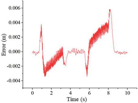
Figure 8 Tracking error with directly compensating dead zone.

6.2 ARC with Flow-mapping Compensator

A flow-mapping compensator is used to compensate for nonlinear flow gain when oil temperature in Kelvin is 313.15 K. The coefficients of the flow gain polynomial are shown as Equation (53).

$$a=\mathrm{\hspace{0.33em}5.957}\times {10}^{-13}b=-2.271\times {10}^{-11}$$
$$c=2.086\times {10}^{-10}d=-1.551\times {10}^{-10}$$	(53)

Figure 9 Tracking error with flow-mapping compensator.

The control voltage is generated by Equation (47). The tracking error is shown in Figure 9. During a movement, the maximum negative error is $-$2.45 mm, and the maximum positive error is 3.1 mm.

7 Conclusions

This paper proposed a controller with a flow-mapping compensator for a PDC valve-controlled cylinder system to improve motion control accuracy for the heavy-load mobile manipulator. The controller is experimentally investigated on a hydraulic robotic manipulator test bench driven by single-rod hydraulic actuators. The control accuracy of using the flow mapping compensator to generate the control voltage is greatly improved than the control accuracy not used. The maximum positive error is only 65.16% of the control accuracy directly compensating the dead zone, and the maximum negative error is only 51.93% of the control accuracy directly compensating the dead zone. The results demonstrate that the control strategy can achieve a higher control accuracy than directly compensating the dead zone.

In the future, we will obtain more data and use machine learning methods to improve the accuracy of the flow-mapping compensator further. Online automatic generation of the flow-mapping compensator is also our goal.

Acknowledgment

This work was supported in part by the National Natural Science Foundation of China (Grant No. 91748210), the National Outstanding Youth Science Foundation of China (Grant No. 51922093), and the National Natural Science Foundation of China (Grant No. 51835009).

References

[1] J. Mattila, J. Koivumaki, D. G. Caldwell, and C. Semini, “A survey on control of hydraulic robotic manipulators with projection to future trends,” IEEE/ASME Trans. on Mechatronics, vol. 22, no. 2. pp. 669–680, 2017.

[2] M. Cheng, J. Zhang, B. Xu, and R. Ding, “An Electrohydraulic Load Sensing System based on flow/pressure switched control for mobile machinery,” ISA Trans., vol. 96, pp. 367–375, 2020.

[3] R. Dindorf and P. Wos, “Force and position control of the integrated electro-hydraulic servo-drive,” Proc. 2019 20th Int. Carpathian Control Conf. ICCC 2019, pp. 1–6, 2019.

[4] M. Han, Y. Song, Y. Cheng, W. Zhao, J. Wei, and X. Ji, “Conceptual Design and Analysis of Water Hydraulic Manipulator for CFETR Blanket Maintenance,” J. Fusion Energy, vol. 34, no. 3, pp. 545–550, 2015.

[5] B. Yao, F. Bu, J. Reedy, and G. T. C. Chiu, “Adaptive robust motion control of single-rod hydraulic actuators: Theory and experiments,” IEEE/ASME Trans. Mechatronics, vol. 5, no. 1, pp. 79–91, 2000.

[6] A. Mohanty and B. Yao, “Indirect adaptive robust control of hydraulic manipulators with accurate parameter estimates,” IEEE Trans. Control Syst. Technol., vol. 19, no. 3, pp. 567–575, 2011.

[7] L. Lyu, Z. Chen, and B. Yao, “Energy Saving Motion Control of Independent Metering Valves and Pump Combined Hydraulic System,” IEEE/ASME Trans. Mechatronics, vol. 24, no. 5, pp. 1909–1920, 2019.

[8] L. Lyu, Z. Chen, and B. Yao, “Development of Pump and Valves Combined Hydraulic System for Both High Tracking Precision and High Energy Efficiency,” IEEE Trans. Ind. Electron., vol. 66, no. 9, pp. 7189–7198, 2019.

[9] Q. Guo, Y. Zhang, B. G. Celler, and S. W. Su, “Backstepping Control of Electro-Hydraulic System Based on Extended-State-Observer with Plant Dynamics Largely Unknown,” IEEE Trans. Ind. Electron., vol. 63, no. 11, pp. 6909–6920, 2016.

[10] J. Zhang, D. Wang, B. Xu, Q. Su, Z. Lu, and W. Wang, “Flow control of a proportional directional valve without the flow meter,” Flow Meas. Instrum., vol. 67, no. October 2018, pp. 131–141, 2019.

Biographies

Fu Zhang received the B.Eng. degree from Jilin University, Changchun, China, in 2018. He is currently working toward the Ph.D. degree in the College of Mechanical Engineering, Zhejiang University, Hangzhou, China. His research interests include hydraulic robots and trajectory planning.

Junhui Zhang received the B.S. degree in 2007 and the Ph.D. degree in 2012, both from Zhejiang University, Hangzhou, China.

He is currently a researcher at the Institute of Mechatronics and Control Engineering, Zhejiang University. His research interests include high-speed hydraulic pumps/motors, hydraulic robots. He published more than 40 papers indexed by SCI, and applied more than 20 National Invention Patents with 18 granted. He is supported by. the National Science Fund for Excellent Young Scholars. He is a technical editor of IEEE/ASME Trans Mechatron.

Bing Xu received the Ph.D. degree in fluid power transmission and control from Zhejiang University, Hangzhou, China, in 2001.

He is currently a Professor and a Doctoral Tutor in the Institute of Mechatronic Control Engineering, and the Director of the State Key Laboratory of Fluid Power and Mechatronic systems, Zhejiang University. He has authored or coauthored more than 200 journal and conference papers and authorized 49 patents. Prof. Xu is a Chair Professor of the Yangtze River Scholars Programme, and a science and technology innovation leader of the Ten Thousand Talent Programme.

Huaizhi Zong received the B.S. degree in 2017 and the M.S. degree in 2020, from Northeastern University, Shenyang and Zhejiang University, Hangzhou, China, respectively. He is currently pursuing the Ph.D. degree in the College of Mechanical Engineering, Zhejiang University, Hangzhou, China. His research interests include hydraulic robots, lightweight design of hydraulic cylinder/accumulator/system, heat transmission, energy recovery and utilization.

International Journal of Fluid Power, Vol. 22_2, 259–276.
doi: 10.13052/ijfp1439-9776.2225
© 2021 River Publishers

Abstract

1 Introduction

2 Dynamic Models

3 Controller Design

4 Flow-Mapping Compensator and Directly Compensating Dead Zone

4.1 Flow-Mapping Compensator

4.2 Directly Compensating Dead Zone

5 Simulation Results

6 Experimental Results

6.1 ARC with Directly Compensating Dead Zone

6.2 ARC with Flow-mapping Compensator

7 Conclusions

Acknowledgment

References

Biographies