Stability Analysis of Spools with Imperfect Sealing Gap Geometries

Rituraj Rituraj* and Rudolf Scheidl

Institute of Machine Design and Hydraulic Drives, Johannes Kepler University, Linz, Austria

E-mail: rituraj.rituraj@jku.at; rudolf.scheidl@jku.at

*Corresponding Author

Received 05 December 2020; Accepted 06 December 2020; Publication 06 February 2021

Abstract

Spools in hydraulic valves are prone to sticking caused by unbalanced lateral forces due to geometric imperfections of their sealing lands. This sticking problem can be related to the stability of the coaxial spool position. Numerical methods are commonly used to study this behaviour. However, since several parameters can influence the spool stability, parametric studies become significantly computationally expensive and graphical analysis of the numerical results in multidimensional parameter space becomes difficult.

To overcome this difficulty, in this work, an analytical approach for studying the stability characteristics of the spool valve is presented. A Rayleigh-Ritz method is used for solving the Reynolds equation in an approximate way in order to determine an analytical expression for the lateral force on the sealing lands. This analytical expression allows stability analysis of the spool via analytical means which finally results in the expression of critical axial velocity which demarcates the regions of stable behaviour. Simplicity of the expression allows an immediate insight into the role of design parameters in the stability of the spool. To verify the analytical model, a numerical model for spool dynamics is developed in this work and the numerical results are found to match the analytical model in terms of the stability behaviour of the spool.

Keywords: Spool valves, sealing gap, Rayleigh-Ritz method, Reynolds equation.

1 Introduction

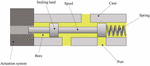
Spool valves are key components in hydraulic systems which are used to control the direction the fluid flow by combining or switching the paths through which the hydraulic fluid can travel. These valves consist of a spool with two or more sealing lands connected by a central spool axle as shown in Figure 1. Clearances in the order of few microns exist between the sealing lands and the valve bore which allows the spool to move with minimal friction while also enabling the sealing lands to perform the sealing function with acceptable leakage.

Figure 1 Typical spool valve.

In an ideal world, the spool sealing lands are perfectly cylindrical, and the spool remains coaxial with respect to the valve bore during operation. However, in reality, the sealing lands suffer from geometric imperfections owing to manufacturing errors. Further, clearances at the sealing lands may allow the spool to move away from its coaxial position. These seemingly small deviations from the ideal scenario result in high radial forces on the spool. In the best-case scenario, these forces stabilize the spool back to the coaxial position. However, in the worst-case scenario, the radial forces destabilize the spool position and press the spool into the bore wall. The latter scenario results in the valve sticking phenomenon [1] (also referred to as hydraulic locking) which is highly undesirable. A classical solution to mitigate this phenomenon is to machine pressure balancing circumferential grooves on the sealing land [2, 3]. However, it remains a topic of interest to study these radial forces and determine the geometric and operating conditions that may lead to an inherently stable behaviour of the spool motion. This forms the goal of this research work.

Researchers in the past have investigated the radial forces on spools and the sticking phenomenon via different means starting from the experimental investigations by Sweeney [4]. Blackburn et al. [5] and Merritt [6] proposed analytical approaches based on 1D assumptions (the flow in the gap between the sealing land and the valve bore was assumed to be axial) to estimate the pressure field in the fluid film around the sealing lands and, thus, the radial force on the spool. The approach was further improved by Viersma [7] by taking peripheral flow into consideration. However, fully accurate solutions for the pressure field in such a fluid film can only be determined by using 2D form of Reynolds equation of lubrication [8] as demonstrated by Borghi [9] and Milani [10].

Nevertheless, a key challenge with current approaches of using the Reynolds equation for such problems is the fact that the equation must be solved via numerical methods, especially when the geometric imperfections exist and/or when the spool is eccentric and tilted with respect to the valve bore. This is due to the presence of the non-uniform conductivity term in the equation which is given by the third power of the gap height. However, critical limitations of such numerical methods are exposed in the parametric study procedures aimed at establishing the stability characteristics of the spool. In particular, there are several parameters that potentially influence the dynamic behaviour of the spool such as the nominal clearance, pressure difference, spool axial velocity and additional parameters characterizing the geometric imperfections. A complete parametric study, then, involves several numerical simulations which are computationally expensive. Furthermore, comprehension of results via graphical representations become cumbersome owing to the parameter space dimensionality.

To overcome these challenges, the authors propose an alternate approach based on analytical methods. Recently, the authors presented a closed form solution for radial forces on stationary spools with sealing lands exhibiting conicity errors [11]. The solution was obtained by employing Rayleigh-Ritz method [12] on 2D Reynolds equation. In this work, the authors extend this approach to non-stationary spools, i.e. spools with axial, radial and angular motions. Further, from the analytical solution of radial force, the conditions for the dynamic stability of spools are determined. The closed form analytical nature of this result makes the influence of the relevant parameters obvious. The results obtained from this analytical approach are verified by a numerical model (also developed in this work) where Reynolds equation and spool dynamics equations are numerically solved.

This paper is structured into 5 sections including this introduction section. In Section 2, the analytical model for the radial force on the spool is obtained via the Rayleigh-Ritz method. Section 3 presents the stability analysis of the spool valve with two sealing lands. In Section 4, details of the numerical model are presented, and the analytical predictions of spool stability are verified. Finally, the summary and key conclusions of the paper are provided in Section 5.

2 Analytical Model for Radial Force on Spool

2.1 Gap Geometry at the Sealing Land

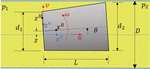
Figure 2 shows a sealing land in a spool bore that is offset from the bore axis by a distance $z$ and is tilted by an angle $\theta$. Further, the sealing land exhibits a conical shape. As shown in Figure 2, the diameter at one end of the sealing land is $d_1$, whereas, the diameter on the other end is $d_2(\ne d_1)$. The conicity of the sealing land can be defined as

$$k=\frac{d_2-d_1}{L}$$

(1)

Figure 2 Geometry and position of the sealing land in a spool valve considered in this work. The coordinate systems for the valve bore and the sealing land are ($x^G,y^G,z^G$) and ($x^B,y^B,z^B$), respectively.

For such a geometric configuration, the height of the gap between the sealing land and the valve bore is

$$h=h_0-\frac{kx}{2}-(\theta x+z)\cos \varphi$$

(2)

where $h_0$ is the nominal radial gap height ($h_0=(D-d_1)/2$), $x$ is the axial coordinate and $\varphi$ is the azimuthal coordinate (from $+z$ axis). Detailed derivation of the gap height expression is present in Ref. [11].

2.2 Variational Form of the Reynolds Equation and Ritz Approximation

As the gap height between the sealing land and the valve bore is of the order of few microns, the pressure in the fluid film in this gap is governed by Reynolds equation of lubrication:

$$\frac{\partial }{\partial x}\left(\frac{h^3}{\eta }\frac{\partial p}{\partial x}\right)+\frac{\partial }{R^2\partial \varphi }\left(\frac{h^3}{\eta }\frac{\partial p}{\partial \varphi }\right)+6u\frac{\partial h}{\partial x}-12\frac{\partial h}{\partial t}=0$$

(3)

where, $R=D/2$, $u$ is the axial velocity of the spool and

$$\frac{\partial h}{\partial t}=-(\omega x+v)\cos \varphi$$

(4)

where, $\omega$ and $v$ are the angular and linear velocities of the sealing land, respectively (also indicated in Figure 2).

The Reynolds equation (Equation (3)) can be transformed into the following variational form:

$\delta \mathrm{\Pi }=0;\mathrm{\Pi }$	$={\displaystyle {\int }_0^{2\pi }}{\displaystyle {\int }_0^L}{\displaystyle \frac{h^3}{\eta }}{\left({\displaystyle \frac{\partial p}{\partial x}}\right)}^2+{\displaystyle \frac{h^3}{R^2\eta }}{\left({\displaystyle \frac{\partial p}{\partial \varphi }}\right)}^2$
	$\mathrm{\hspace{1em}}-12u{\displaystyle \frac{\partial h}{\partial x}}p+24{\displaystyle \frac{\partial h}{\partial t}}pdxd\varphi$	(5)

The existence of a variational formulation allows the usage of Rayleigh-Ritz method to obtain the best approximation of the solution. In this case, the following Ritz ansatz is used to describe the pressure field:

$p(x,\varphi )=a_{00}+a_{01}{\displaystyle \frac{x}{L}}+a_{02}{\left({\displaystyle \frac{x}{L}}\right)}^2+\left(a_{10}+a_{11}{\displaystyle \frac{x}{L}}+a_{12}{\left({\displaystyle \frac{x}{L}}\right)}^2\right)\cos \varphi$

(6)

Employing the boundary conditions: $p(x=0)=p_1,p(x=L)=p_2$, the pressure expression simplifies to:

$$p(x,\varphi )=p_1+\frac{p_2-p_1}{L}x+\left(\frac{x^2}{L^2}-\frac{x}{L}\right)\left(a_{02}+a_{12}\cos \varphi \right)$$

(7)

The coefficients $a_{02}$ and $a_{12}$ can be determined by invoking the stationarity of $\mathrm{\Pi }$ (in Equation (5)) with respect to these coefficients, i.e.

$$\frac{\partial \mathrm{\Pi }}{\partial a_{02}}=0;\frac{\partial \mathrm{\Pi }}{\partial a_{12}}=0$$

(8)

The resulting expressions of $a_{02}$ and $a_{12}$ are lengthy and hence, are not shown here. However, the smallness of $k$, $z$, $\theta$, $v$, $\omega$ allows us to take a truncated Taylor series of the solutions with respect to these variables up to the first non-vanishing order. This results in the following compact expressions for $a_{02}$ and $a_{12}$:

$a_{02}$	$={\displaystyle \frac{3k\lambda \left(R\mathrm{\Delta }p{\mu }^2+0.5\eta \lambda u\right)}{8{\mu }^{3}R}}$	(9)
$a_{12}$	$={\displaystyle \frac{15\lambda \left[R\theta k{\mu }^2\lambda +{\mu }^2\left(4\theta \mu +kz\right)\right]\mathrm{\Delta }p}{8R{\mu }^4\left({\lambda }^2+10\right)}}$
	$\mathrm{\hspace{1em}}+{\displaystyle \frac{\begin{array}{c}15\eta {\lambda }^2[\lambda \omega (3k\lambda +8\mu )R^2\hfill \\ +(-6k(\theta u-v)\lambda -8\mu (\theta u-2v))R-6kuz]\hfill \end{array}}{32R^2{\mu }^4({\lambda }^2+10)}}$	(10)

where $\lambda =L/R$, $\mu =h_0/D$ and $\mathrm{\Delta }p=p_2-p_1$.

2.3 Force and Torque Evaluation

The pressure field (Equation (7)) can be integrated over the fluid film to obtain the force acting on the sealing land. As the pressure is symmetric with respect to the $x-z$ plane, there is no force in $y$ direction (into the page as per Figure 2). As $k$ and $\theta$ are very small, the axial force (in $x$ direction) is negligible. The force in $z$ direction is:

$F_z$	$=-{\displaystyle {\int }_0^L}{\displaystyle {\int }_0^{2\pi }}pR\cos \varphi \mathit{d}\varphi \mathit{d}x$	(11)
$\Rightarrow F_z$	$={\displaystyle \frac{5\lambda \pi L}{64R{\mu }^4\left({\lambda }^2+10\right)}}\{(3{\lambda }^3\eta k{R}^2+8R^2\eta \mu {\lambda }^2)\omega$
	$\mathrm{\hspace{1em}}+(-6R\eta ku{\lambda }^2+(-4R^{2}k\mathrm{\Delta }p{\mu }^2-8R\eta u\mu )\lambda -16{\mu }^3{R}^2\mathrm{\Delta }p)\theta$
	$\mathrm{\hspace{1em}}+(6{\lambda }^2\eta kR+16R\eta \mu \lambda )v+(-6\eta k\lambda u-4Rk{\mu }^2\mathrm{\Delta }p)z\}$	(12)

2.3.1 Special case: Steady state conditions

For the steady state scenario, i.e., $u=v=\omega =0$, the force expression becomes:

$F_z={\displaystyle \frac{5\pi \mathrm{\Delta }p\lambda L\left(R\theta k\lambda +4\theta R\mu +kz\right)}{16{\mu }^2\left({\lambda }^2+10\right)}}$

(13)

From this result, following interpretations about the spool stability can be drawn:

• For parallel displacement ($z\ne 0,\theta =0$), the spool is stable if $k\mathrm{\Delta }p<0$. The resulting force is always in the direction opposite to the parallel displacement, pulling the spool back to its central position.

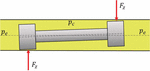
• For perfect sealing land ($k=0$), a parallel displacement ($z\ne 0,\theta =0$) does not result in any force. On the other hand, any tilt with a negative $\mathrm{\Delta }p$ results in a stabilizing force. This means that, in the case of a spool with two perfect sealing lands with the pressures shown in Figure 3, the spool is always stable if $p_c>p_e$ and unstable if $p_c<p_e$.

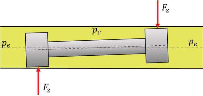
Figure 3 Tilted spool with two perfect sealing lands is stable if $p_c>p_e$.

2.3.2 General case: unsteady conditions

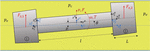
To analyse the dynamic behaviour of the spool, the net force and torque on the spool with multiple sealing lands must be determined. In this work, a spool with two sealing lands is considered, the geometric parameters of which are illustrated in Figure 4.

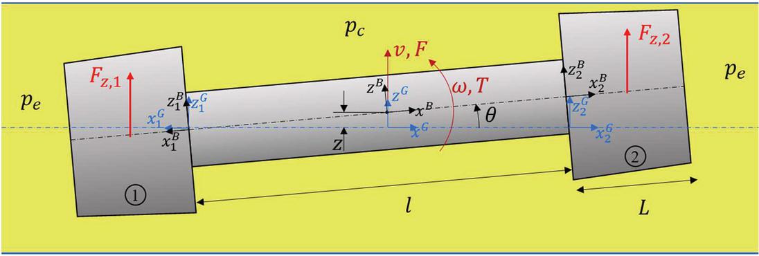
Figure 4 Geometry and position of a spool with two sealing lands considered in this work. The coordinate systems for the valve and the spool are specified by superscripts $G$ and $B$, respectively.

Here, the net force and net torque are

$F=F_{z,1}+F_{z,2};T=0.5(L+l)(F_{z,2}-F_{z,1})$

(14)

Where $F_{z,1}$ and $F_{z,2}$ are determined from Equation (12) by applying appropriate coordinate transformations. In particular, the coordinate transformations for $F_{z,1}$ are:

${\theta }_1=-\theta ;{\omega }_1=-\omega ;z_1=z-{\displaystyle \frac{\theta l}{2}};v_1=v-{\displaystyle \frac{\omega l}{2}};u_1=-u$

and that for $F_{z,2}$ are:

${\theta }_2=\theta ;{\omega }_2=\omega ;z_2=z+{\displaystyle \frac{\theta l}{2}};v_2=v+{\displaystyle \frac{\omega l}{2}};u_1=u$

The expressions for $F$ and $T$ are reported below:

$F=F_z\cdot z+F_{\theta }\cdot \theta +F_v\cdot v+0\cdot \omega$

(17)

where,

$F_z$	$={\displaystyle \frac{5\pi L\lambda k\mathrm{\Delta }p}{8{\mu }^2\left({\lambda }^2+10\right)}}$	(18)
$F_{\theta }$	$={\displaystyle \frac{5\pi L{\lambda }^2\eta u}{8R{\mu }^4\left({\lambda }^2+10\right)}}\left\{{\displaystyle \frac{3}{2}}Rk\lambda +2R\mu +{\displaystyle \frac{3}{4}}kl\right\}$	(19)
$F_v$	$={\displaystyle \frac{5\pi L{\lambda }^2\eta }{8{\mu }^4\left({\lambda }^2+10\right)}}\left\{-{\displaystyle \frac{3}{2}}k\lambda -4\mu \right\}$	(20)
$T$	$=T_z\cdot z+T_{\theta }\cdot \theta +0\cdot v+T_{\omega }\cdot \omega$	(21)

where,

$T_z$	$={\displaystyle \frac{15\pi L{\lambda }^2\eta ku(L+l)}{32R{\mu }^4({\lambda }^2+10)}}$	(22)
$T_{\theta }$	$={\displaystyle \frac{5\pi L\lambda (L+l)\mathrm{\Delta }p}{32{\mu }^2({\lambda }^2+10)}}\{2Rk\lambda +8R\mu +kl\}$	(23)
$T_{\omega }$	$=-{\displaystyle \frac{5\pi L{\lambda }^2\eta (L+l)}{64{\mu }^4({\lambda }^2+10)}}(3k\lambda +8\mu )(R\lambda +l)$	(24)

It is to be noted that in above expressions, the conicities of the two sealing lands are assumed to be identical and mirrored with respect to the centre of the spool (e.g. both sealing lands in Figure 4 have negative conicity).

3 Stability Analysis of the Spool Dynamics

The system of equations governing the spool motion is

$\left[\begin{array}{cc}\hfill m\mathit{\hspace{1em}}\hfill & \hfill 0\hfill \\ \hfill 0\mathit{\hspace{1em}}\hfill & \hfill J\hfill \end{array}\right]\left(\begin{array}{c}\hfill \ddot{z}\hfill \\ \hfill \ddot{\theta }\hfill \end{array}\right)=\left(\begin{array}{c}\hfill F\hfill \\ \hfill T\hfill \end{array}\right)$

(25)

Substituting Equations (17) and (21) in above system of equations,

$\left[\begin{array}{cc}\hfill m\mathit{\hspace{1em}}\hfill & \hfill 0\hfill \\ \hfill 0\mathit{\hspace{1em}}\hfill & \hfill J\hfill \end{array}\right]\left(\begin{array}{c}\hfill \ddot{z}\hfill \\ \hfill \ddot{\theta }\hfill \end{array}\right)+\left[\begin{array}{cc}\hfill -F_v\mathit{\hspace{1em}}\hfill & \hfill 0\hfill \\ \hfill 0\mathit{\hspace{1em}}\hfill & \hfill -T_{\omega }\hfill \end{array}\right]\left(\begin{array}{c}\hfill \dot{z}\hfill \\ \hfill \dot{\theta }\hfill \end{array}\right)+\left[\begin{array}{cc}\hfill -F_z\mathit{\hspace{1em}}\hfill & \hfill -F_{\theta }\hfill \\ \hfill -T_z\mathit{\hspace{1em}}\hfill & \hfill -T_{\theta }\hfill \end{array}\right]\left(\begin{array}{c}\hfill z\hfill \\ \hfill \theta \hfill \end{array}\right)=0$

(26)

3.1 Effect of Inertia Terms

To assess the significance of the inertia terms, following non-dimensionalisation is adopted:

$z=\zeta h_0;\theta =\beta {\displaystyle \frac{h_0}{L}};J=\tilde{J}\left|\mathrm{\Delta }p\right|\pi t_e^2{l}^{2}L;u=\tilde{u}{\displaystyle \frac{s}{t_e}};s=\sigma R;$
$m=\tilde{m}L|\mathrm{\Delta }p|\pi t_e^2;k=\tilde{k}{\displaystyle \frac{h_0}{L}};l=\tilde{l}R;\eta =\tilde{\eta }|\mathrm{\Delta }p|t_e{\mu }^2;t=\tau t_e$	(27)

The resulting system of equations is:

$\left[\begin{array}{cc}\hfill \widehat{m}\mathit{\hspace{1em}}\hfill & \hfill 0\hfill \\ \hfill 0\mathit{\hspace{1em}}\hfill & \hfill \widehat{J}\hfill \end{array}\right]\left(\begin{array}{c}\hfill {\zeta }^{\prime \prime }\hfill \\ \hfill {\beta }^{\prime \prime }\hfill \end{array}\right)+\left[\begin{array}{cc}\hfill {\widehat{F}}_{\dot{\zeta }}\mathit{\hspace{1em}}\hfill & \hfill 0\hfill \\ \hfill 0\mathit{\hspace{1em}}\hfill & \hfill {\widehat{T}}_{\dot{\beta }}\hfill \end{array}\right]\left(\begin{array}{c}\hfill {\zeta }^{\prime }\hfill \\ \hfill {\beta }^{\prime }\hfill \end{array}\right)+\left[\begin{array}{cc}\hfill {\widehat{F}}_{\zeta }\mathit{\hspace{1em}}\hfill & \hfill {\widehat{F}}_{\theta }\hfill \\ \hfill {\widehat{T}}_{\zeta }\mathit{\hspace{1em}}\hfill & \hfill {\widehat{T}}_{\beta }\hfill \end{array}\right]\left(\begin{array}{c}\hfill \zeta \hfill \\ \hfill \beta \hfill \end{array}\right)=0$

(28)

where,

${()}^{\prime }$	$={\displaystyle \frac{d}{d\tau }}()$	(29)
$\widehat{m}$	$=\tilde{m}\mu ;\widehat{J}=\tilde{J}{\tilde{l}}^2\mu$	(30)
${\widehat{F}}_{\dot{\zeta }}$	$={\displaystyle \frac{5{\lambda }^2\tilde{\eta }(3\tilde{k}+4)}{8({\lambda }^2+10)}};{\widehat{F}}_{\zeta }=-{\displaystyle \frac{5\tilde{k}sign(\mathrm{\Delta }p)}{4({\lambda }^2+10)}};$
${\widehat{F}}_{\theta }$	$=-{\displaystyle \frac{5\sigma \tilde{u}\tilde{\eta }\{(3\tilde{k}+2)\lambda +1.5\tilde{k}\tilde{l}\}}{8({\lambda }^2+10)}}$	(31)
${\widehat{T}}_{\dot{\beta }}$	$={\displaystyle \frac{5{\lambda }^2\tilde{\eta }(3\tilde{k}+4){(\tilde{l}+\lambda )}^2}{32({\lambda }^2+10)}};{\widehat{T}}_{\zeta }=-{\displaystyle \frac{15{\lambda }^2\tilde{\eta }\tilde{k}\sigma \tilde{u}(\tilde{l}+\lambda )}{16({\lambda }^2+10)}};$
${\widehat{T}}_{\beta }$	$=-{\displaystyle \frac{5(\tilde{l}+\lambda )sign(\mathrm{\Delta }p)\left\{(\tilde{k}+2)\lambda +0.5\tilde{k}\tilde{l}\right\}}{8({\lambda }^2+10)}}$	(32)

It is notable that all the terms are $\sim \mathit{O}(1)$ except the inertia terms where $\mu$ is present. As $\mu =h_0/D=\mathit{O}({10}^{-3})$, the inertia terms play little role in the dynamic behaviour of the spool motion. Thus, inertia terms will be neglected in the analysis going forward. This step significantly simplifies the analytical computations in the next subsection and allows final closed form expressions for the stability of the system.

3.2 Conditions for the Stability of the Spool

Upon neglecting the inertia terms, the system of equations (Equation (28)) transform into the following form:

$\mathit{D}\mathit{X}{}^{\mathbf{\prime }}+\mathit{K}\mathit{X}=0$	(33)
$\mathbf{\Rightarrow }\mathit{X}{}^{\mathbf{\prime }}=(-{\mathit{D}}^{-1}\mathit{K})\mathit{X}$	(34)

Now, the dynamical properties of this system are fully characterized by the eigenvalues of the matrix $-{\mathit{D}}^{-1}\mathit{K}$, which are determined to be:

${\mathrm{\Lambda }}_{1,2}={\displaystyle \frac{A\pm \sqrt{B+C{\tilde{u}}^2}}{G}}$

(35)

where,

$A$	$=sign(\mathrm{\Delta }p)(2\tilde{k}\tilde{l}+3\tilde{k}\lambda +4\lambda )$	(36)
$B$	$={\lambda }^2{(\tilde{k}+4)}^2$	(37)
$C$	$=3{\tilde{\eta }}^2\tilde{k}{\lambda }^2{\sigma }^2(\tilde{l}+\lambda )(3\tilde{k}\tilde{l}+6\tilde{k}\lambda +4\lambda )$	(38)
$G$	$=\tilde{\eta }{\lambda }^2(\tilde{l}+\lambda )(3\tilde{k}+4)$	(39)

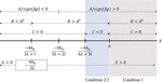
For real valued eigenvalues, the stability of the system requires ${\mathrm{\Lambda }}_{1,2}<0$. This is satisfied for the following two conditions:

$\mathrm{\#}1.\mathit{\hspace{1em}}A<0,B<A^2,C>0,G>0,-\sqrt{{\displaystyle \frac{A^2-B}{C}}}<\tilde{u}<\sqrt{{\displaystyle \frac{A^2-B}{C}}}$	(40)
$\mathrm{\#}2.\mathit{\hspace{1em}}A<0,B>A^2,C<0,G>0,\{\begin{array}{c}\hfill -\sqrt{-{\displaystyle \frac{B}{C}}}<\tilde{u}<-\sqrt{{\displaystyle \frac{A^2-B}{C}}}\hfill \\ \hfill \sqrt{{\displaystyle \frac{A^2-B}{C}}}<\tilde{u}<\sqrt{-{\displaystyle \frac{B}{C}}}\hfill \end{array}$	(41)

These conditions essentially put certain limits on the axial velocity of the spool for different geometric and operating conditions to ensure a stable behaviour. The conditions on variables $A,B,C,G$ specified in Equations (40) and (41) are mainly driven by the value of conicity and hence, it is better to visualize these conditions with respect to the conicity parameter (Figure 5). The figure shows that when $k>0$, the requirements on all the variables imposed in condition 1 are automatically satisfied (except the sign of $A$). On the other hand, for $k<0$, requirements on all the variables imposed in condition 2 are satisfied as long as $k>-4h_0/(6L+3l)$. One exception is the negativity requirement for $A$ in these conditions which demands a negative $\mathrm{\Delta }p$ (i.e. $p_c>p_e$ in Figure 4).

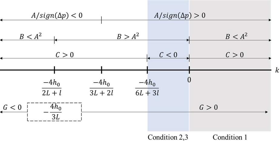
Figure 5 Regions of stability conditions with respect to conicity $k$. Within each region, the axial velocity limits of Equations (40) and (41) need to be satisfied to ensure stability. $G=0$ location depends on the relative values of $L$ and $l$.

A third condition can be obtained by considering the case of complex eigenvalues (i.e. ${\tilde{u}}^2>-B/C$). In this case, the stability of the system is ensured when $C<0$ and $A/G<0$. As per Figure 5, when $C<0$, $G>0$. Thus, $A$ needs to be negative to ensure $A/G<0$. On inspection, this condition is identical to condition 2 (Equation (41)) in terms of the ranges of $A,B,C,G$. Thus, condition 2 and 3 can be combined to obtain the following:

$\mathrm{\#}2.\mathit{\hspace{1em}}A<0,B>A^2,C<0,G>0,\{\begin{array}{c}\hfill \tilde{u}<-\sqrt{{\displaystyle \frac{A^2-B}{C}}}\hfill \\ \hfill \tilde{u}>\sqrt{{\displaystyle \frac{A^2-B}{C}}}\hfill \end{array}$

(42)

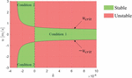
The stability conditions obtained in previous paragraphs are summarized in Figure 6. For positive conicity, if the magnitude of the axial spool velocity remains under a critical value ($u_{crit}$), the spool will exhibit a stable behaviour. On the other hand, for negative conicity, the spool velocity needs to be higher than this critical value to ensure stability. The expression of the critical axial velocity is

$u_{crit}=\sqrt{{\displaystyle \frac{A^2-B}{C}}}={\displaystyle \frac{|\mathrm{\Delta }p|h_0^2}{6L\eta }}\sqrt{{\displaystyle \frac{(2L+l)k+4h_0}{(2L+l)k+\frac{4}{3}{h}_0}}}$

(43)

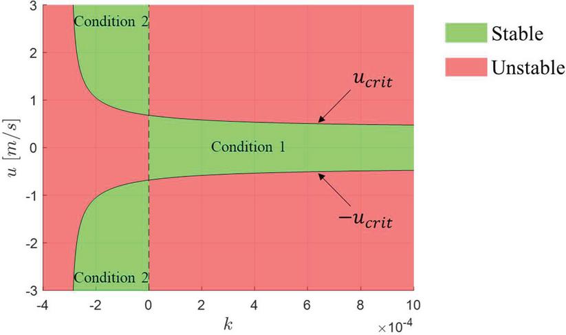
Figure 6 Stability map in $k-u$ parameter space. Parameter values chosen to obtain this plot: $\mathrm{\Delta }p=-99$ bar, $h_0=10$ $\mu$m, $L=15$ mm, $l=15$ mm, $\eta =0.028$ Pas.

This analytical formulation for critical axial velocity is a significant outcome of this research. The simple formula clearly establishes the relationships between parameters such as height of the gap, length of the spool, pressure difference, fluid viscosity and the critical axial velocity. This formulation along with the stability map (Figure 6) is enough to describe the stability characteristics of a spool valve with two sealing lands.

It is notable that although both conditions, 1 and 2, lead to the stable behaviour of the spool, only condition 1 encompasses $u=0$ (stationary spool). Thus, from the practical point of view, condition 1 gives a useful range of operation for the spool valves.

4 Verification with a Numerical Model

A numerical model for spool dynamics is developed in this work to verify the stability predictions from the analytical model. The numerical model consists of a finite difference model for the determination of pressure in the fluid film around the sealing lands of the spool. This model is coupled with the spool dynamics model for the determination of instantaneous position and velocity (linear and angular) of the spool.

4.1 Finite Difference Model

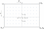
The fluid film around the sealing land is unwrapped and discretized into $N_x$ points in $x$ direction (axial direction) and $N_{\varphi }$ points in $\varphi$ direction (circumferential direction) as shown in Figure 7. A finite difference method is employed on the Reynolds equation (Equation (3)) to obtain the following set of algebraic equations:

${\displaystyle \frac{h_{i,j}^3}{\mathrm{\Delta }{x}^2}}{p}_{i-1,j}+{\displaystyle \frac{h_{i,j}^3}{R\mathrm{\Delta }{\varphi }^2}}{p}_{i,j-1}-\left\{{\displaystyle \frac{h_{i,j}^3+h_{i+1,j}^3}{\Delta x^2}}+{\displaystyle \frac{h_{i,j}^3+h_{i,j+1}^3}{R\Delta {\varphi }^2}}\right\}{p}_{i,j}$
$\mathrm{\hspace{1em}\hspace{1em}}+{\displaystyle \frac{h_{i,j+1}^3}{\Delta x^2}}{p}_{i,j+1}+{\displaystyle \frac{h_{i+1,j}^3}{\Delta x^2}}{p}_{i+1,j}=-6\eta u{\left({\displaystyle \frac{\partial h}{\partial x}}\right)}_{i,j}+12\eta {\left({\displaystyle \frac{\partial h}{\partial t}}\right)}_{i,j}$	(44)

where,

${\left({\displaystyle \frac{\partial h}{\partial x}}\right)}_{i,j}=-{\displaystyle \frac{k}{2}}-\theta \cos {\varphi }_j;{\left({\displaystyle \frac{\partial h}{\partial t}}\right)}_{i,j}=-(\omega x_i-v)\cos {\varphi }_j$

(45)

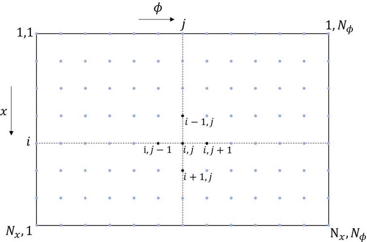
Figure 7 Discretization of the unwrapped fluid film.

Equation (44) is a system of linear equation in $p_{i,j}$ applicable for all the points in the computational grid except for $\{(1,j),(N_x,j)|j\in \{1,\mathrm{\dots },N_{\varphi }\}\}$ points where the pressures are known from the boundary conditions ($p(x=0)=p_c,p(x=L)=p_e$ as per Figure 4). The system of equations is solved to obtain the pressures at all the grid points.

4.2 Equations of Motion Model and Solver

The pressure at the grid points is numerically integrated via 2D trapezoidal method to determine the force in $z$ direction and the torque with respect to the centre of the spool. The integrand for the force calculation is $-pR\cos \varphi$, whereas that for the torque calculation is $-(l/2+x)pR\cos \varphi$.

If $F_{z,1},T_1$ and $F_{z,2},T_2$ are the force-torque pairs calculated for the sealing lands 1 and 2 in Figure 4, then, the net force on the spool is $F=F_{z,1}+F_{z,2}$ and the net torque on the spool is $T=-T_1+T_2$. The opposite signs of $T_1$ and $T_2$ come from the mirrored orientation of the coordinate system for sealing lands 1 and 2 in Figure 4.

The equation of motion for the spool dynamics is then solved implicitly in time to account for the small inertial effect which gives the system a high stiffness:

${\mathit{X}}^n-{\mathit{X}}^{n-1}-\Delta t{\mathcal{ℱ}}^n=0$

(46)

where,

$\mathit{X}=\left\{\begin{array}{c}\hfill v\hfill \\ \hfill z\hfill \\ \hfill \omega \hfill \\ \hfill \theta \hfill \end{array}\right\};\mathcal{ℱ}=\left\{\begin{array}{c}\hfill F/m\hfill \\ \hfill v\hfill \\ \hfill T/J\hfill \\ \hfill \omega \hfill \end{array}\right\}$

(47)

Table 1 Simulation cases used to compare the analytical and numerical results

Case	1	2
$L$	15 mm
$D$	10 mm
$l$	15 mm
$h_0$	10 $\mu$m
$p_c$	100 bar
$p_e$	1 bar
$\eta$	0.028 Pas
$k$	$0.000267$	$-0.000267$
Stability prediction from	$-0.56<u<0.56$ (m/s)	$u<-1.81$ m/s, $u>1.81$ m/s
analytical model

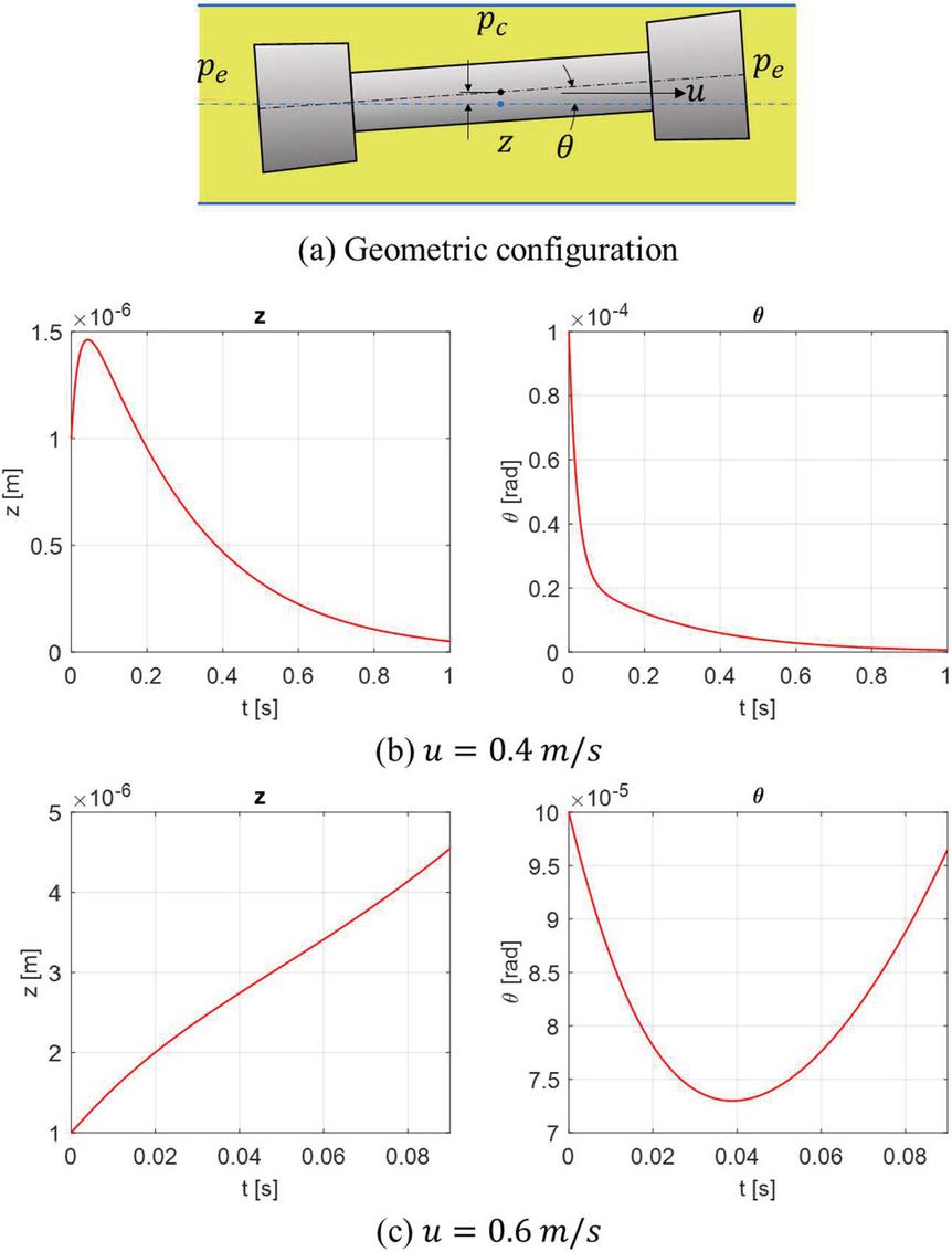
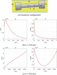
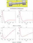
Figure 8 Evolution of the spool position with time for simulation case 1 in Table 1.

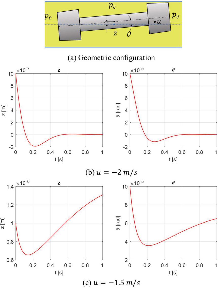
Figure 9 Evolution of the spool position with time for simulation case 2 in Table 1.

4.3 Results from the Numerical Model and Comparison with Analytical Prediction

The numerical model described in the previous subsections is used to conduct simulations to study the stability behaviour of the spools. Table 1 shows the simulation cases that represent the two conditions for stability presented in Section 3.2. Simulations are conducted with a small initial perturbation of the spool ($z=1$ $\mu$m, $\theta ={10}^{-4}$ rad) from its coaxial position.

For simulation case 1, as per the analytical model, the spool is stable for $-0.56<u<0.56$ (m/s). Figure 8 shows the temporal evolution of the spool position for this case with two axial velocities $u=0.4$ m/s and $u=0.6$ m/s, the former lying in the stability region and the latter outside. From the figure, it is clear that the spool goes to its coaxial position when $u=0.4$ m/s, whereas it goes away from the coaxial position when $u=0.6$ m/s. This is consistent with the analytical prediction.

Similarly, for simulation case 2, the analytical model predicts stability in the range: $u<-1.81$ m/s and $u>1.81$ m/s. To verify this, simulations were conducted for $u=-2$ m/s and $u=-1.5$ m/s. The temporal evolution of the spool position for these two axial velocities is presented in Figure 9. The results show that the spool is stable for $u=-2$ m/s and unstable for $u=-1.5$ m/s, which is again consistent with the analytical prediction.

5 Summary and Conclusions

Spool valves often suffer from the dynamic instability of the spool with respect to its coaxial position in the valve bore. This results in the spool sticking to the bore walls causing large sticking forces. This phenomenon is significantly affected by the geometric imperfections (arising from manufacturing errors) in the sealing lands of the spool.

In this work, the stability of the spool valves with geometric imperfection in the form of conicity error on the sealing lands is investigated via analytical methods. A Rayleigh-Ritz method is employed on the Reynolds equation of lubrication to determine an analytical expression of the radial force on the sealing lands. From this information, the net force and torque on a spool with two sealing lands is evaluated and a stability analysis is conducted to determine the conditions for the stable behaviour of the spool motion.

The analysis indicates that for positive conicity error, the spool will be stable if the magnitude of spool axial velocity stays under a critical value. On the other hand, for negative conicity error, the spool will be stable if the magnitude of spool axial velocity remains higher than a critical value. In this work, these findings have been verified via a numerical model for the spool valve dynamics.

The analytical model developed in this work has a key advantage in terms of the simplicity of the stability conditions. The model proposes simple analytical formulations for spool stability which allows a compact understanding of the role of design parameters. Thus, it can be easily used by valve designers in developing spool valves with better stability characteristics, for instance, by a proper conical shaping of the sealing lands.

Nomenclature

$D$	Diameter of the valve bore
$d$	Diameter of the spool sealing land
$F$	Force
$h$	Height of the gap between the sealing land and the valve bore
$J$	Moment of inertia of the spool
$k$	Conicity of the spool sealing land
$l$	Distance between the two sealing lands
$L$	Width of the spool sealing land
$m$	Mass of the spool
$p$	Pressure
$R$	Radius of the valve bore
$T$	Torque
$t$	Time
$u$	Axial velocity of the spool
$v$	Velocity of the spool along $+z$ direction
$x$	Coordinate direction along the axis of the valve
$z$	Radial offset of the spool with respect to the valve bore axis
Greek letters
$\eta$	Fluid viscosity
$\theta$	Angular offset of the spool with respect to the valve bore axis
$\mathrm{\Lambda }$	Eigenvalue
$\lambda$	L/R
$\mu$	$h_0$/D
$\mathrm{\Pi }$	Functional of the variational problem
$\varphi$	Azimuthal coordinate from $+z$ axis
$\omega$	Angular velocity of the spool
Superscripts
$B$	Spool body frame of reference
$G$	Ground frame of reference
Subscripts
$c$	Center
$e$	Edge
$o$	Nominal
$1,2$	Identifier for the sealing lands

Acknowledgement

This work was done in the framework of the COMET K2 Center on Symbiotic Mechatronics, which is funded by the Austrian Federal Government, the State Upper Austria and by its Scientific and Industrial Partners.

References

[1] B. Winkler, G. Mikota, R. Scheidl, B. Manhartsgruber, Modeling and simulation of the elasto-hydrodynamic behavior of sealing gaps, Aust. J. Mech. Eng. 2 (2005) 65–72. https://doi.org/10.1080/14484846.2005.11464481.

[2] T.-J. Park, Y.-G. Hwang, Effect of Groove Sectional Shape on the Lubrication Characteristics of Hydraulic Spool Valve, Tribol. Online. 5 (2010) 239–244. https://doi.org/10.2474/trol.5.239.

[3] S.H. Hong, K.W. Kim, A new type groove for hydraulic spool valve, Tribol. Int. 103 (2016) 629–640. https://doi.org/10.1016/j.triboint.2016.07.009.

[4] D.C. Sweeney, Preliminary investigation of hydraulic lock, Engineering. 172 (1951) 513–516.

[5] Blackburn, J. F., G. Reethof, J.L. Shearer, Fluid Power Control, MIT Press-John Wiley, New York, 1960.

[6] H.E. Merritt, Hydraulic Control Systems, John Wiley & Sons, Inc., New York, 1967.

[7] T.J. Viersma, Analysis, synthesis, and design of hydraulic servosystems and pipelines, Elsevier, Amsterdam, 1980.

[8] B.J. Hamrock, S.R. Schmid, B.O. Jacobson, Fundamentals of fluid film lubrication, CRC Press, 2004.

[9] M. Borghi, Hydraulic locking-in spool-type valves: Tapered clearances analysis, Proc. Inst. Mech. Eng. Part I J. Syst. Control Eng. 215 (2001) 157–168. https://doi.org/10.1243/0959651011540941.

[10] M. Milani, Designing hydraulic locking balancing grooves, Proc. Inst. Mech. Eng. Part I J. Syst. Control Eng. 215 (2001) 453–465. https://doi.org/10.1177/095965180121500503.

[11] R. Scheidl, M. Resch, M. Scherrer, P. Zagar, An approximate, closed form solution of sealing gap induced lateral forces for imperfect sealing land geometries, in: Int. Sci. Tech. Conf. NSHP 2020, Wrocław, Poland, 2020.

[12] T. Zheng, S. Yang, Z. Xiao, W. Zhang, A ritz model of unsteady oil-film forces for nonlinear dynamic rotor-bearing system, J. Appl. Mech. Trans. ASME. 71 (2004) 219–224. https://doi.org/10.1115/1.1640369.

Biographies

Rituraj Rituraj received his B.Tech. degree from IIT Guwahati, India in 2013 and his Ph.D. degree from Purdue University, USA in 2020. During his direct-Ph.D. at Maha Fluid Power Research Center, he worked on numerical modelling of External Gear Machines. Currently, he is a postdoctoral researcher at Institute of Machine Design and Hydraulic Drives in JKU, Austria. His research interests include numerical and experimental study of hydraulic components and systems.

Rudolf Scheidl received his M.Sc. of Mechanical Engineering and Doctor of Engineering Sciences degrees at Vienna University of Technology. He has research and development experience in agricultural machinery (Epple Buxbaum Werke), continuous casting technology (Voest-Alpine Industrieanlagenbau) and paper mills (Voith). Since 1990, he is a full Professor of Mechanical Engineering at Johannes Kepler University, Austria. His research topics include hydraulic drive technology and mechatronic design.

International Journal of Fluid Power, Vol. 21_3, 383–404.
doi: 10.13052/ijfp1439-9776.2135
© 2020 River Publishers

Abstract

1 Introduction

2 Analytical Model for Radial Force on Spool

2.1 Gap Geometry at the Sealing Land

2.2 Variational Form of the Reynolds Equation and Ritz Approximation

2.3 Force and Torque Evaluation

2.3.1 Special case: Steady state conditions

2.3.2 General case: unsteady conditions

3 Stability Analysis of the Spool Dynamics

3.1 Effect of Inertia Terms

3.2 Conditions for the Stability of the Spool

4 Verification with a Numerical Model

4.1 Finite Difference Model

4.2 Equations of Motion Model and Solver

4.3 Results from the Numerical Model and Comparison with Analytical Prediction

5 Summary and Conclusions

Nomenclature

Acknowledgement

References

Biographies