CFD Assisted Steady-State Modelling of Restrictive Counterbalance Valves

Jannik H. Jakobsen* and Michael R. Hansen

Department of Engineering Sciences, Faculty of Engineering and Science, University of Agder, Jon Lilletunsvei 9, 4879 Grimstad, Norway

Email: jannik.jakobsen@uia.no

* Corresponding Author

Received 26 July 2019; Accepted 25 May 2020; Publication 23 June 2020

Abstract

The counterbalance valve is an important component in many hydraulic applications and its behaviour hugely impacts system stability and performance. Despite that, CBVs are rarely modelled accurately due to the effort required to obtain basic model parameters and the complexity involved in identifying expressions for flow forces and friction. This paper presents a CFD assisted approach to steady-state modelling of CBVs. It is applied to a 3-port restrictive commercially available counterbalance valve. The model obtained is based on detailed measurements of the valve geometry, a single data set and CFD modelling and includes flow forces and friction. The CFD assisted model is compared to experimental data at three temperatures and two versions of more classical steady-state model based on the orifice equation, uniform pressure distribution and experimental results. The results support the CFD assisted approach as a way to increase modelling accuracy. The load pressure corrected coulomb friction model used manages to capture the changes to hysteresis with temperature but not the changes with pilot pressure.

Keywords: Valve modelling, friction modelling; counterbalance valve; hydraulics; computational fluid dynamics; steady state characteristics.

Introduction

The counterbalance valve, CBV, also known as the overcenter valve, is an important component in many hydraulic applications. Leak tight load-holding is required by law in almost all hydraulic load-carrying applications and the CBV provides this and a number of other functionalities without the need for electrical control. This includes cavitation protection when moving assisting loads (typically load lowering situations), protection of the mechanical system against overloading in general, and shock loading in particular. Furthermore, the CBV normally acts as a line rupture safety valve, i.e., it provides load holding if there is a loss of pressure in either or both of the main supply lines. It is, therefore, directly fitted to the hydraulic actuator with no hose or piping in between. On top of these important functionalities, the advantage of the CBV is that it reduces the meter in pressure dependency on the payload load. This advantage means, that for almost any hydraulically actuated machinery with loads that vary substantially and are both resistive and assistive, the CBV is easily the preferred choice.

The main disadvantage associated with the use of a CBV is that when combined with a pressure compensated directional control valve, PCDCV, the result is often a highly oscillatory system. This tendency becomes more pronounced at small velocities and with high pilot area ratio CBVs.

Various methods have been suggested for dealing with the issue such as negative flow forces (Hansen, et al., 2004), various forms of feedback compensation, and modifications to the PCDCV (Sørensen, et al., 2016). Most of these methods have limited effect, work only on a case by case basis and/or increase system energy consumption and cost.

Other methods widely used in industry (Sørensen, 2016) include the forced opening of the CBV leaving the return flow throttling required to control motion of assisting loads to the return orifice of the PCDCV. Alternatively, the pressure compensator of the PCDCV may be forced open or a constant pressure source may be added to the metering in flow. These solutions do, however, have serious shortcomings reducing either the ability to handle even modest variations in assistive loads or removing the pressure compensated flow and thereby the controllability.

Ideally, it should be possible to predict the oscillatory behaviour of a system containing a CBV and a PCDCV. Unfortunately, the valve parameters available for a system designer are typically not accurate enough to support the development of a model that can predict this type of behaviour. In fact, even steady-state characteristics that are crucial to any kind of hydraulic analysis can be difficult to obtain with commercially available documentation.

Why do we need to improve the existing models of CBVs?

In addition to the lack of information in the valve documentation, modelling both the friction and flow force is non-trivial.

The CBV differs from most valves by being more strongly affected by piston friction related to the need for anti-leakage (Handroos & Vilenius, 1993).

The friction is non-linear and rather complex since it may depend on both velocity, velocity history, oil type, temperature, pressure and surface roughness. The flow force has similarly been shown to have a significant effect on CBV behaviour (Hansen, et al., 2004) and a high level of complexity (Handroos & Halme, 1996).

Studies with a semi empirical determined friction force (Miyakawa, 1978) and with both a semi-empirical determined friction and a flow force (Persson, et al., 1989) and (Handroos & Halme, 1996) exist but all of these approaches are limited in scope and are targeting specific CBVs.

Determining the flow force in CBVs can be difficult. Simple analytical expressions can be derived (Merrit, 1967), but they may be inaccurate (Handroos & Halme, 1996). The flow force can, alternatively, be determined empirically, but it can rarely be measured directly and must often be derived from the piston kinetics through experiments. However, for CBVs the influence from the relatively large friction force obscures the results and decrease the accuracy of the identified flow force expression.

CFD is a common tool used to investigate flow force in valves and it has been used in (Hansen, et al., 2004) (Amirante, et al., 2006) to investigate how valve design effects flow force. In (Yuan & Li, 2005) CFD results have been directly compared to force measurements and successfully used to determine an expression for flow force on a flow valve.

In this paper, a new method for modelling the steady-state characteristics of CBVs is presented. It is a CFD assisted method that requires a single dataset and detailed information on the geometry of the valve. The main objective is to allow for the correct prediction of the valve flow, the flow force and the piston friction force for any combination of operating conditions. It is especially well suited for the restrictive CBV version covered in the paper, as the main piston experiences a relatively large flow force.”

What is the benefit of CFD assisted modelling?

If the flow force and the friction force are ignored or modelled in an overly simplified way, then the model cannot accurately predict the valve flow and the corresponding pressure drop for the full range of operating conditions.

Having a CFD model help distinguishing the model components from each other and, therefore, increase accuracy, when identifying friction by fitting the model to the data.

Using CFD also allows for identification of the flow force with dependencies on a broad spectrum of parameters. Both dependencies on state parameters like temperature and pilot pressure but also oil type dependant parameters like density and viscosity can be determined with no or limited testing.

Nomenclature

Variables generally start with lower case and constants starts with upper case letters.

αP	Pilot ratio
αL	Liquid fraction
αfront	Front fraction
AB	Effective area, back pressure
AL	Effective area, load pressure
AP	Effective area, pilot pressure
As3	Effective area, in the spring chamber
BM	Basic model
BMBE	Basic effort model
BMBEBF	Basic effort best fit model
Cd	Discharge coefficient
CV	Relative flow coefficient
CBV	Counterbalance valve
CFD	Computational fluid dynamics
CFDA	CFD assisted model
δ	Relative piston position
Δp	Pressure difference across valve
Fcr	Crack force
fff	Flow force
ffl	Fluid force
fμ	Friction force
fsim	Fluid force from CFD model
fspr	Spring force
K1	Friction coefficient
K2	Friction coefficient
Kf	Spring coefficient
Kδ	Relative spring coefficient
ρ	Fluid density
p	Pressure
Pcr	Crack pressure
pL	Load pressure
pB	Back pressure
pP	Pilot pressure
Pvap.oil	Evaporation pressure
psat	Saturation pressure
PCDCV	Pressure compensated directional control valve
φ	Cylinder area ratio
q	Flow
qin	Flow delivered by PCDCV
qsim	Flow from CFD model
Re	Reynolds number
s	Sign of ụ
u	Piston position
Umax	Maximum piston position
vG	Gas volume
vL	Liquid volume
w	Discharge area coefficient

Considered CBV

In this study, a single commercial 3-port CBV is used as an example. It is characterized as a restrictive CBV with non-axisymmetric flow access to its main restriction. The behaviour is somewhat atypical and the use of CFD assisted modelling is, therefore, especially relevant for this type of CBV.

The three ports are called back-, pilot- and load-port. The CBV valve has two primary modes of operation. It operates as a check valve when flow is sent from the back-port to the load-port, and acts as a piloted open relief valve, when flow is sent from the load-side to the back-side. This article focuses on modelling the piloted open relief valve functionality.

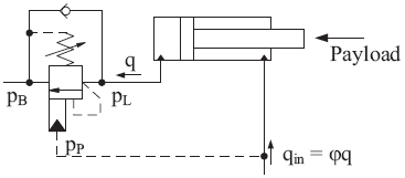
Figure 1 Simplified load-holding circuit consisting of a 3-port CBV and a cylinder.

Figure 2 A cross-section of the CBV. Piston at u=0 mm and poppet seated on piston. The blue arrows indicate the flow direction.

Figure 1 shows a simplified load-holding circuit, where the flow, q, is restricted by the CBV, which acts as a piloted open relief valve.

When the CBV acts as a piloted open relief valve, the load pressure, p_L, and the pilot pressure, p_P, will tend to open the valve, while the back pressure, pb, and the spring force will tend to close it. The initial spring compression will normally be set to accommodate a crack pressure specified to be a certain percentage above the maximum allowable p_L. When q_in, see Figure 1, is supplied by a PCDCV, p_P and p_L will adjust to allow the flow through the CBV to be q =q_in/φ, where φ is the cylinder area ratio.

In Figures 2 and 3 a cross-section of the valve used for this study is shown. The two main moving components are the piston and the poppet. The poppet along with the minor spring ensures the check valve function and allow flow through the main restriction towards the load side by moving to the left. The piston ensures the pilot operated relief function by moving to the right, while the poppet is prevented from moving right by the poppet stop. This allows flow through the main restriction.

Figure 3 shows the various pressure regions, that govern the piston movement, and the respective effective areas on which they act at u = 0 mm and Table 1 lists the relevant effective cross sectional areas. α_P is the pilot ratio. The back chamber and main spring chamber are in the same pressure region, but a distinction is made, as the main spring chamber is not modelled in the CFD model introduced below.

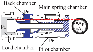
Figure 3 A cross-section of the CBV, with pressure indications, and effective cross-sectional areas.

Table 1 Measured effective cross-sectional piston areas. The pilot ratio is α_P=A_P/A_L = 2.72

Parameter	Value
AL	10.7 mm2
AP	αPAL
AB	(αP+1) AL

Figure 4 shows three cross-sections of the valve inlet. The valve inlet geometry is not axisymmetric and the oil can only flow to the main restriction via the upper and bottom channel shown in cross-section G-G. This makes it more difficult for the flow to reach the parts of the main restriction not located near the upper or lower channel as oil will both have to travel further and change direction to get there. The limited flow access to the main restriction causes the valve to be more restrictive than typical CBVs.

Valve Model

The steady-state valve behaviour can be described by two main equations, one describing how much flow passes through the valve at a given pressure differential and piston position, (1), and one describing the force equilibrium on piston, (2).

$$\mathrm{q}=\mathrm{f}({\mathrm{p}}_{\mathrm{L}},{\mathrm{p}}_{\mathrm{B}},\mathrm{u},\mathrm{R}\mathrm{e})$$

(1)

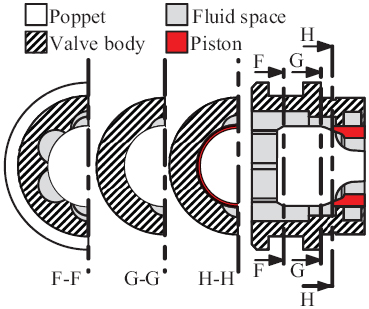
Figure 4 Valve cross-section which illustrates the lack of axisymmetry in the restricted flow inlet.

Where Re is the Reynolds number.

$$0={\mathrm{f}}_{\mathrm{f}\mathrm{l}}-{\mathrm{f}}_{\mu }{-\mathrm{f}}_{\mathrm{s}\mathrm{p}\mathrm{r}}$$

(2)

Where f_fl is the force transferred to the piston from the fluid, f_μ is the friction force acting on the piston from the piston track and seals and f_spr is the force acting on the piston from the springs.

The spring force takes the form of (3)

$${\mathrm{f}}_{\mathrm{s}\mathrm{p}\mathrm{r}}={\mathrm{F}}_{\mathrm{c}\mathrm{r}}+{\mathrm{K}}_{\mathrm{f}}\mathrm{u}$$

(3)

Where F_cr = 226 N is the force from the springs at u = 0 mm, and K_f = 1.14e5 Nm⁻¹ is the spring constant.

Table 2 describes the remaining components of (1) and (2) for two models. The first is referred to as the basic model (BM) and the second is the model introduced in this paper, referred to as the CFD assisted model, CFDA. BM is a lump-parameter model based on the standard orifice equation and the standard force equilibrium obtained from uniform pressure distributions.

The CFDA model supplements the lump parameter model with components found with CFD simulations of the valve. The idea is to map post-processed results from CFD simulations to improve the accuracy of q in (1) and f_fl in (2).

Table 2 Model components of BM and CFDA BM CFDA

	BM	CFDA
q	${\displaystyle {\mathrm{C}}_{\mathrm{d}}{\mathrm{a}}_{\mathrm{d}}\sqrt{\frac{2}{\rho }({\mathrm{p}}_{\mathrm{L}}-{\mathrm{p}}_{\mathrm{B}})}}$ (4)	qsim(pL, pB, u) (5)
ffl	pLAL+pPAP−pBAB (6)	fsim (pL, pB, u) − pBAs3+pPAP (7)
fμ	0	s(K1+K2pL) (8)

The BM uses the classic orifice equation (4). The discharge coefficient C_d is assumed constant, and the discharge area, a_d is considered a linear function of the piston travel u.

$$a_d=\mathrm{w}\cdot \mathrm{u}$$

(9)

Where w is the discharge area coefficient.

The force equilibrium of the standard model assumes all pressurized areas on the piston to be either affected by p_L, p_P or p_B and disregards flow forces. Where flow force is defined as the force produced by flow (Merrit, 1967). It can be calculated as the difference between the fluid forces produced by the terms of (6) and the actual fluid force.

$${\mathrm{f}}_{\mathrm{f}\mathrm{f}}={\mathrm{f}}_{\mathrm{f}\mathrm{l}.\mathrm{a}\mathrm{c}\mathrm{t}\mathrm{u}\mathrm{a}\mathrm{l}}-{\mathrm{f}}_{\mathrm{f}\mathrm{l}.\mathrm{B}\mathrm{M}}$$

(10)

The CFDA model uses CFD simulation at various combinations of q and u across the range of expected operating conditions to map the relationship between q, p_L, p_b and u. The flow found in CFD simulations is named q_sim. Similarly, the CFD is used to map the fluid forces on the piston (7) which by default includes flow forces. The fluid force from the CFD model is named f_sim. To reduce the computations necessary for simulation not all of the fluid in contact with the piston is modelled. The flow to the piston areas in the main spring chamber and pilot chamber is expected to be small and are not near the main restriction, therefore, a uniform pressure distribution is assumed in both of these volumes. Their contributions to the force equilibrium are added as separate terms in (7), where A_s3 is the effective piston area in the spring chamber. Note that A_s3>A_B.

The CFD assisted model uses the empirical determined Coulomb friction model of (Handroos & Halme, 1996) (8), where s is sign(ụ) and K₁ and K₂ are found using the hysteresis of a dataset.

Using CFD to model the valve comes at a cost as more information and model work is needed. To compare effort against the increased accuracy, the CFDA model will be compared with two versions of the BM that represent two levels of effort and accuracy.

Basic effort – BMBE

The BM can be transformed into a model of only three valve dependent parameters, α_P, C_V and K_δ:

$$\mathrm{q}={\mathrm{C}}_{\mathrm{V}}\delta \sqrt{\mathrm{\Delta }\mathrm{p}}$$

(11)

$$\delta =\frac{{\mathrm{p}}_{\mathrm{L}}+{\alpha }_{\mathrm{P}}\cdot {\mathrm{p}}_{\mathrm{P}}-\left({\alpha }_{\mathrm{P}}+1\right){\mathrm{p}}_{\mathrm{B}}-{\mathrm{P}}_{\mathrm{c}\mathrm{r}}}{{\mathrm{K}}_{\delta }}$$

(12)

(Bak & Hansen, 2013)

Where d is the relative piston position d= u/U_max, P_cr is the crack pressure, P_cr=F_cr/A_L, Δ_p = p_L − p_B and C_V and K_δ are related to C_d and K_f as follows:

$${\mathrm{C}}_{\mathrm{v}}={\mathrm{C}}_{\mathrm{d}}\mathrm{w}{\mathrm{U}}_{\mathrm{m}\mathrm{a}\mathrm{x}}\sqrt{\frac{2}{\rho }}$$

(13)

$${\mathrm{K}}_{\delta }=\frac{{\mathrm{K}}_{\mathrm{f}}{\mathrm{U}}_{\mathrm{m}\mathrm{a}\mathrm{x}}}{{\mathrm{A}}_{\mathrm{L}}}$$

(14)

The value of α_P is obtainable from the valve datasheet, C_V is the relative flow coefficient. It can typically be derived from the piloted open curve (q,Δp) in the datasheet. K_δ is the relative spring coefficient. It may be derived from a no pilot pressure (q,Δp) curve sometimes found in datasheets or may come directly from the manufacturer (Bak & Hansen, 2013).

The BMBE model of this article emulates the use of a piloted open curve and K_δ given by the manufacturer. To make comparisons between models easier emulation is done by setting C_d and K_f instead of identifying C_v and K_δ directly. C_d is found at u=0.63mm to be between 0.3 to 0.4 (see Figure 12) for most flows and temperatures. C_d = 0.4 is chosen for the model. K_f is measured to be 1.14e5 Nm⁻¹. A C_d value of 0.4 is alow value. As explained in the section CFD, it is a result of the restrictive nature of the chosen CBV type.

Basic effort best fit – BMBEBF

Often, the only way to get the information needed is to test and fit the curves to a data set. Combining (11) and (12) into (15) shows that q is proportional to the C_V/K_δ-ratio and therefore fitting either C_V or K_δ to a data set leads to the same model.

$$\begin{array}{r}\mathrm{q}=\frac{{\mathrm{C}}_{\mathrm{V}}}{{\mathrm{K}}_{\delta }}\sqrt{\mathrm{\Delta }\mathrm{p}}\cdot ({\mathrm{p}}_{\mathrm{L}}+{\alpha }_{\mathrm{P}}\cdot {\mathrm{p}}_{\mathrm{P}}-\left({\alpha }_{\mathrm{P}}+1\right){\mathrm{p}}_{\mathrm{B}}-{\mathrm{P}}_{\mathrm{c}\mathrm{r}})\end{array}$$

(15)

In the BMBEBF model, the fitting scenario is therefore emulated by fitting C_d to a dataset at a temperature of 40°C while using the measured K_f.

Listing the needed information for the three models looks like this:

Table 3 Model information needed for valve parameters of the three models

Information	BMBE	BMBEBF	CFDA
αP	x	x
Piloted open curve	x
No pilot pressure curve/ Kδ from manufacturer	x
Test curve with known pP		x	x
Valve geometry			x
Spring measurements			x

CFD

The mesh is generated from a CAD geometry. As mentioned above the pilot chamber and the main spring chamber is not modelled. Of the remaining fluid volume only a quarter needs to be modelled since two planes of symmetry exist. At the very end of the outlet the valve is not actually symmetric (see Figure 2), but this have little influence on the flow at the main restriction and the outlet geometry has, therefore, been modified in the CFD model to keep the two symmetry planes and reduce the number of computations needed for each simulation.

The fluid geometry is based on detailed measurements obtained with a precision calliper and macro photography. This setup allows a precision tolerance down to ±0.01 mm. The valve is relatively small and accuracy of this order of magnitude is needed at the main restriction with the width of the A_L surface being 0.43 mm and the main edge radius around 0.03 mm.

One mesh is created for each simulated u. the values simulated are:

$$\mathrm{u}\in \left\{0.05,0.08,0.10,0.13,0.16,0.20,0.63\right\}\text{mm}$$

The Siemens Star CCM+ software is used to create a polyhedral mesh with 6 prism layers. The polyhedral mesh is chosen over a tetrahedral mesh for an improvement in convergence speed. The 6 prism layers reduces the cell count while still maintaining a sufficiently small first cell height ensuring a well-resolved boundary layer.

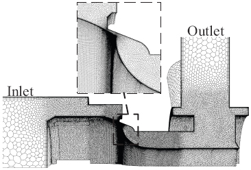
Figure 5 Mesh used for the u=0.1 mm simulations.

Table 4 Relative Δp change with refinement increasing from 1.7M to 3.1M cells for u=0.1 mm

q [L/min]	1	3	6	9	12
Δ(Δp) [%]	1.53	1.86	-0.88	-1.64	-1.84

Figure 5 shows the manually added cell refinement as it increases towards the restriction where the turbulent energy, fluid velocities and fluid pressure experience gradients are orders of magnitude higher than in the remainder of the model.

The refinement and, subsequently, the total cell count varies depending on u. Small u leads to a smaller gap at the main restriction and smaller cells are required to resolve the gap. The total cell count for the produced meshes varied from 1.6 to 4.3M cells.

Table 4 shows the effect on simulation results of scaling the refinement uniformly across the mesh for the 0.10 mm geometry. The table suggests result changes of less than 2% on Δp, and it is not deemed worth the extra computational time to increase the refinement beyond a cell count of 3.1M.

The oil used for the experiments is Shell Tellus S2 V46. It is a standard VG46 HV (ISO) oil type. The main CFD model components are the SST K-omega turbulence model and the Schnerr-Sauer cavitation model. The model components were chosen based on available data and documented success with similar problems. (Valdés, et al., 2014) achieved good results and accuracy with the SST-k-omega turbulence model and the Schnerr-Sauer cavitation model on water flow through a ball check valve.

Oil cavitation is, however, different from water in that cavitation happens in stages. First, dissolved air begins to be released from the fluid at

$$\mathrm{p}<{\mathrm{p}}_{\mathrm{s}\mathrm{a}\mathrm{t}}=1.0\mathrm{b}\mathrm{a}\mathrm{r}$$

(gas cavitation) and then the oil starts evaporating at (typical hydraulic oil):

$$\mathrm{p}<{\mathrm{p}}_{\mathrm{v}\mathrm{a}\mathrm{p}.\mathrm{o}\mathrm{i}\mathrm{l}}=0.3\mathrm{b}\mathrm{a}\mathrm{r}$$

(Casoli, et al., 2006). This means that if the oil is treated as a fluid evaporating at either p_sat or p_vap.oil the actual degree of cavitation is expected to be in between the two scenarios.

Both scenarios were simulated with less than 0.25% difference on Δp and 1.06% on f_sim for u = 0.1 mm, q = 12 L/min and 40°C. For simplicity, the general simulations are run with P_vap = P_sat = 1 bar and with gas properties like air.

The effect of cavitation is more pronounced at higher flows. For the case of u = 0.1 mm, q = 12 L/min, Δp was 9% higher and f_sim 24% higher when compared to a similar model with no cavitation component and a fixed minimum pressure of 0 bar. Figure 6 shows a comparison of f_sim across the entire q-u-map at 40°C.

The multi-phase mixture model is used, the liquid is assumed incompressible, isothermal and at steady state. Figures 7–9 depict the results from a single CFD simulation at u=0.1 mm, q=6 L/min and 40°C.

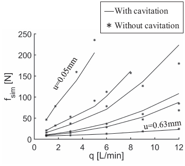
Figure 6 f_sim(q) simulations at 40°C with (−) and without (*) cavitation component. Constant u curves from top-left to bottom-right 0.05, 0.08, 0.10, 0.13, 0.16, 0.20 and 0.63 [mm].

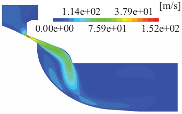
Figure 7 Simulation results. Velocity magnitude [m/s] contours of the main restriction and flow after. u=0.1 mm, q=6 L/min and temperature is 40°C.

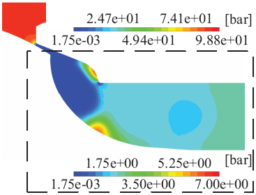
Figure 8 Simulation results. Pressure [bar] contours of the main restriction and flow after. u = 0.1 mm, q = 6 L/min and temperature is 40°C. Pressure scale in box differs from outside. Scaling inside the box reveals zones, that are above and below p_b and, therefore, contribute to the flow force.

α_L is the liquid fraction given by (16):

$${\alpha }_{\mathrm{L}}=\frac{{\mathrm{v}}_{\mathrm{L}}}{{\mathrm{v}}_{\mathrm{G}}+{\mathrm{v}}_{\mathrm{L}}}$$

(16)

Where v_L is the volume of liquid and v_G the volume of gas.

Figure 7 shows very high velocities mid-stream at the main restriction and a swirl after. Figure 8 shows high pressures before the restriction and a pressure region immediately after the restriction below p_sat. Figure 9 shows a low liquid fraction on a large part of the piston surface near the main restriction and in the centre of the swirl.

Figure 9 Simulation results. Liquid fraction, α_L [-] contours of the main restriction and flow after. u=0.1 mm, q=6 L/min and temperature is 40°C.

The high velocity stream produces below p_sat pressures regions, which in turn causes cavitation and accumulation of gas in the regions with low velocity and low pressure and therefore a reduction of the liquid fraction, α_L, in those regions. The cavitation influences the forces on the piston and the pressure drop by reducing the cross-sectional area which effectively carries liquid (mass).

The limited access to the main restriction, see Figure 4, has a significant impact on valve characteristics. Both the forces on the piston and the flow through the main restriction is affected. Figure 10 shows how it causes an uneven distribution of pressure along the orifice and load side surface of the piston.

At the top of the cross section (red zone), the pressure is close to the inlet pressure but the pressure drops to less than 53% as the distance to the flow path of section G-G increases (green zone).

Without the CFD model or other investigations, uniform pressure would be assumed on the full front piston surface, which would lead to a significant error in the force on the surface and, therefore, on the error of the valve model.

Figure 11 shows the effect of the uneven pressure distribution on the force on the piston front of Figure 10 as a function of q and u. It depicts the front fraction, α_front, the relative difference between the simulated force and the expected force produced by assuming load pressure on the full surface:

$${\alpha }_{\mathrm{f}\mathrm{r}\mathrm{o}\mathrm{n}\mathrm{t}}=\frac{{\mathrm{f}}_{\mathrm{s}\mathrm{i}\mathrm{m}.\mathrm{f}\mathrm{r}\mathrm{o}\mathrm{n}\mathrm{t}}-{\mathrm{p}}_{\mathrm{L}.\mathrm{s}\mathrm{i}\mathrm{m}}{\mathrm{A}}_{\mathrm{L}}}{{\mathrm{p}}_{\mathrm{L}.\mathrm{s}\mathrm{i}\mathrm{m}}{\mathrm{A}}_{\mathrm{L}}}$$

(17)

The flow force is defined as the difference between actual fluid forces and forces from the uniform pressure distribution, see (10). This means that α_front is the relative flow force contribution from the piston front.

Figure 10 Pressure distribution [bar] along the front of the piston surface (red surface on section H-H in Figure 4). u=0.1 mm, q=6 L/min and 40°C. The circumference of the flow path at section G-G of Figure 4 is shown with dashed lines. Note that only a quarter of the full cross section is shown due to symmetry.

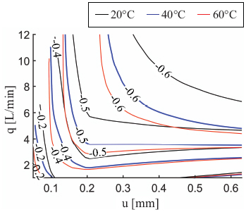
Figure 11 α_front (u, q) plotted as a function of u and q for all three temperatures.

While the piston front surface is not the only surface where a contribution to the flow force can be found, it is, however, home to the main flow force component due to the high pressure on the surface. Figure 11 is, therefore, a reasonable map of the relative flow force predicted by the CFD model.

In general, the CFD model predicts a very large negative flow force. In terms of effects on the model, assuming load pressure on the full surface will for u >0.05 mm lead to a significant overestimation of force on the load side. Less actual forces available means a more restrictive valve and thus less flow at the same load and pilot pressure. For 0.05 mm < u <0.20 mm, which covers most of the workspace, forces reduce primarily with increasing u, reductions starts at 20% and ending at more than 50% reduction for most q. Near u = 0.63 mm and q = 12 L/min the reduction is more than 60%. Temperature also has an effect with higher reductions at lower temperatures.

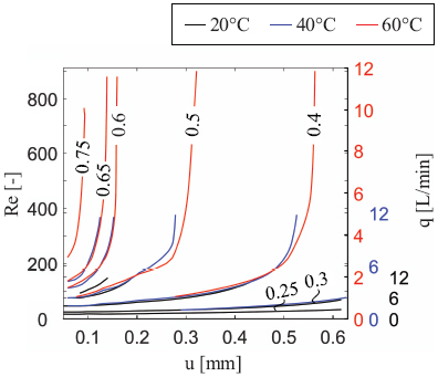
Figure 12 Contours of C_d(u, Re).

Figure 12 shows the simulated C_d-factor as a function of Reynolds number, Re, and u for all three temperatures.

C_d changes significantly with piston position, and the correlation between C_d and Re is in good agreement for all three temperatures. For low Reynolds numbers, Re<50, C_d is mainly a function of Re, and for high Reynolds numbers, C_d is mainly a function of u. Between that there is an intermediate field where for a given u, C_d starts low but grows with Re until it asymptotically approaches a fixed value. For the simulated valve openings, C_d ranges from 0.25 to 0.75, which deviates substantially both in range and lower value compared C_d factors typically found in the literature for simple orifices, which suggests influence from the restricted flow access.

Figures 13 and 14 show the simulation results used for the q_sim and f_sim maps of the CFDA model for all three temperatures. Each curve is a simulation set done with the same u.

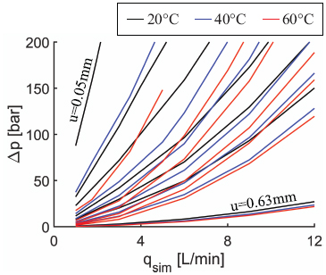
Figure 13 Flow-pressure-position simulation results for the q_sim maps for all three temperatures. u from top-left to bottom-right 0.05, 0.08, 0.10, 0.13, 0.16, 0.20 and 0.63 [mm].

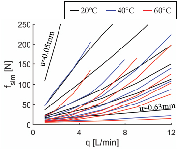
Figure 14 Force-flow-position simulation results for the f_sim maps for all three temperatures. u from top-left to bottom-right 0.05, 0.08, 0.10, 0.13, 0.16, 0.20 and 0.63 [mm].

Figure 13 shows the Δp-q-u maps. The pressure drop, Δp, increases with q but the rate is reduced both with increased valve opening and increased temperature.

Figure 14 shows f_sim as a function of q. The f_sim(q)-curves share the general trends of the Δp(q)-curves.

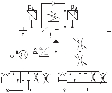
Figure 15 Circuit diagram of the test setup.

Experiments

Setup

The circuit diagram of the test setup is presented in Figure 15.

The pressures at the 3-ports of the valve, the flow through the valve and the temperature of the fluid at the inlet are all measured. Note that the flowmeter is encoder based and inaccurate at very low flow. Data at q < 1 L/min has, therefore, been omitted. The flow through the CBV is controlled using a pressure compensated proportional directional control valve, and the pilot pressure is controlled using a similar valve in series with two adjustable orifices. The power supply is constant pressure at 200 bar with a maximum flow of 15.5 L/min.

The temperature is controlled by placing the entire setup in a refrigerated container and adjusting the ambient air temperature level and letting the oil-to-air heat exchanger of the HPU cool the oil.

The variation of pB throughout the tests due to variation in q and temperature is 1.2 to 7.3 bar. The effective area Ab is a factor (α_P+1) = 3.7 larger than A_L and the Δp(q) curve resulting from constant p_P will, therefore, depend on p_B with a contribution of up to 20.0 bar on Δp. p_P is adjusted to reduce the impact from the p_B variations.

Rewriting (6):

$${\mathrm{f}}_{\mathrm{f}\mathrm{l}}={\mathrm{A}}_{\mathrm{L}}\cdot {\mathrm{p}}_{\mathrm{L}}+{\alpha }_{\mathrm{P}}{\mathrm{A}}_{\mathrm{L}}\cdot {\mathrm{p}}_{\mathrm{P}}-\left({\alpha }_{\mathrm{P}}+1\right){\mathrm{A}}_{\mathrm{L}}\cdot {\mathrm{p}}_{\mathrm{B}}$$

(18)

And defining:

$${\mathrm{p}}_{\mathrm{P}\mathrm{e}}={\mathrm{p}}_{\mathrm{P}}-{\mathrm{p}}_{\mathrm{B}}$$

(19)

Yields:

$${\mathrm{f}}_{\mathrm{f}\mathrm{l}}={\mathrm{A}}_{\mathrm{L}}\mathrm{△}\mathrm{p}+{\alpha }_{\mathrm{P}}{\mathrm{A}}_{\mathrm{L}}\cdot {\mathrm{p}}_{\mathrm{P}\mathrm{e}}$$

(20)

Using p_Pe and Δp eliminates the variable, p_B. It reduces the independent variables during data collection and, therefore, the dimensions of the resulting test matrix. This comes at the cost of not investigating how, p_B, effects flow force and flow coefficients.

This also makes test and characterization of non-vented CBVs like the one modelled in this article similar to vented CBVs (where A_L = A_B). The test sequence is as follows.

• 10–15 s of no flow.
• Ramp up input to PCPDCV to reach 12 L/min over 20 s.
• Ramp down input signal to reach 0 L/min over 20 s.

Test data:

Figure 16 shows the Δp(q) data for all three temperatures. One data set is created for each p_pe value and temperature.

Each dataset consists of a forward curve (upper – 0→12 L/min) and a returning curve (lower – 12→0 L/min) with hysteresis separating the two. The figure shows 4 clusters of similar datasets, one cluster for each test value of p_Pe. Each cluster consists of 3 datasets, one for each temperature tested.

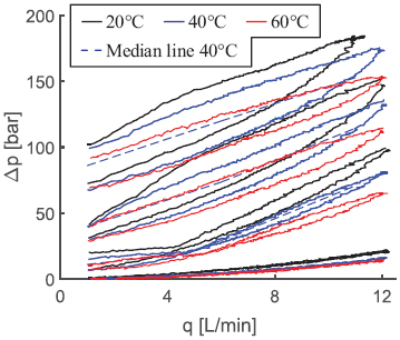
Figure 16 Δp as a function of q, at p_Pe = {50,65,80,120} bar, and at all three temperatures. Datasets from top to bottom is p_Pe = {50; 65; 80,120} bar.

The basic trends are as expected. Higher p_Pe allows the valve to open at lower Δp and both the opening Δp and hysteresis grow with falling temperatures.

To benchmark the models against each other, a median curve similar to the one used in (Handroos & Halme, 1996) is produced. The main purpose of using the median curve is to exclude the influence of friction on the data. Figure 16 shows the median lines for 40°C one for each cluster (p_Pe) effected by hysteresis p_Pe = {50, 65, 80} bar.

Results

The models are compared to the data at each temperature and presented in Figures 17–19. The friction component of the CFDA model is deactivated and the models are compared to the median line of the data to achieve a friction independent benchmark. The accuracy of each model is displayed in Table 5.

The BMBE model fits the data near q = 1 L/min for most p_Pe and temperatures which indicate reasonable estimates of forces and uniform pressure distributions when the valve opens. However, for all other q the rise in Δp with q is grossly underestimated and models a much less restrictive valve than the data suggests.

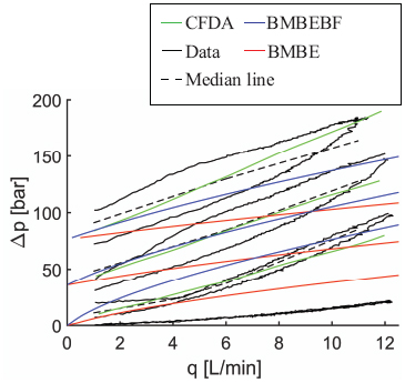
Figure 17 Models vs data at 20°C.

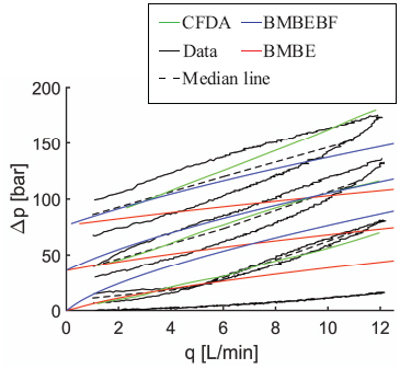
Figure 18 Models vs data at 40°C.

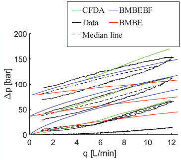
Figure 19 Models vs data at 60°C.

The BMBEBF model can achieve a good fit over a limited temperature and p_Pe range. It is fitted to the p_Pe = 65 dataset at 40°C. The best fit standard model inherits the same properties near q = 1 L/min, and fits most temperatures well at p_Pe = 50 bar and p_Pe = 65 bar. The best fit standard model can, however, not fit the data for p_Pe = 80 bar well while fitting the 50 bar and 65 bar datasets well.

The CFDA model has been adapted to fit the data at 40°C and p_Pe = 65 bar by a 10% reduction of the simulated flow force.

Table 5 Model accuracy. Accuracy is measured as the average distance from the median line and simplified into categories

pPe [bar]	50			65			80
Temperature [°C]	20	40	60	20	40	60	20	40	60
BMBE	−	−	−	−	−	−	−	−	−
BMBEBF	−	++	++	+	+	−	−	−	−
CFDA	+	+	−	++	++	+	+	+	+
“−” more than 15 bar from the median line. “+” more than 10 bar from the median line. “++” less than 5 bar from the median line.

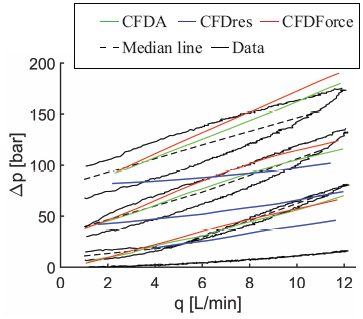
Figure 20 Models vs data at 40°C.

The model fits well across all temperatures and most p_Pe with a slight overestimation of Δp at 20°C. It does so with a better match of the slope and by following the data temperature trends (higher Δp at low temperature).

The CFD simulations improve the model accuracy compared to the BM models in two ways. The first is by the mapping of q_sim followed by replacing the standard orifice equation (4) with the maps (equivalent to correcting C_d). The second is by mapping f_sim(including flow forces) and replacing the uniform pressure distribution terms of (6). The separate contributions of the two ways are investigated in Figure 20.

Figure 20 shows the two curves CFDAForce and CFDARes.

CFDAForce shows the prediction obtained with a CFDA model that only includes the mapping of f_sim but uses the standard orifice equation, while the CFDARes curve shows the prediction obtained with a CFDA model that includes mapping of q_sim but only uses the uniform pressure distributions of equation (6). The figure shows that the f_sim mapping (including flow force) contribute significantly more to accuracy than the q_sim maps (C_d corrections).

Both maps contribute positively to model accuracy and are needed to achieve the results in Table 5.

Friction

Including the term for the friction force allow for direct comparison with the data rather than the derived median lines and makes it possible to determine the characteristics of the friction force. Figure 21 shows the CFDA model with its friction component against the data at 40°C.

Very limited piston movement happens during the p_Pe = 80 bar dataset, according to the Δp-q-u-map from the CFD simulations. This explains the disappearance of the hysteresis near q = 5 L/min and the model’s overestimation of the friction for this dataset.

Figure 21 shows a fit to the p_Pe = 65 bar dataset. It shows that the hysteresis predicted at p_Pe = 50 bar is underestimated. It was not possible to find a set of constants, K₁ and K₂, that model the hysteresis at both p_Pe = 50 bar and p_Pe = 65 bar in a satisfactory way. Table 6, therefore, includes constants for fits to both datasets.

The data demonstrates higher valve hysteresis at lower temperatures, and this is reflected in the models K₁ friction coefficients. The relative increase in K₁ with temperature is similar for both datasets, but the absolute difference between the p_Pe = 65 bar fit is 23–28% less than the p_Pe = 50 bar fit. K₂ does not change much with temperature or dataset.

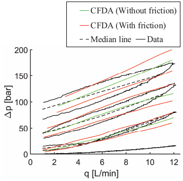
Figure 21 CFDA model with and without the friction component at 40°C. Fit to the p_Pe=65 bar dataset.

Table 6 K₁ and K₂ for 20°C, 40°C and 60°C fitted to the two datasets p_pe = 50 bar and p_Pe = 65 bar.

	pPe = 65 bar		pPe = 50 bar
	K1 [N]	K2 [10−2N/bar]	K1 [N]	K2 [10−2N/bar]
20°C	10	5	13.0	5
40°C	6.5	5	10	5
60°C	5.0	4	6.5	4

A significant difference between the hysteresis predicted and the hysteresis in the data suggests unmodeled friction on the piston. This could, for example, be a component describing the effect of the pilot pressure on the friction. The K₁ coefficient does, however, predict the relative change of hysteresis between temperatures well.

Conclusions

A method for using CFD analysis to improve steady-state modelling of CBV valves has been proposed. It is compared with two basic models where one requires a minimum of information (basic effort, BMBE) and the second requires experimental work (basic effort – best fit, BMBEBF). The CFD assisted model (CFDA) is based on the mapping of the flow-pressure characteristics of the main restriction of the valve and the mapping of the resultant forces on the piston from the fluid. The mapping depends on piston travel and Reynolds number or flow and is set up to cover the range of operating conditions of the valve.

The CFD simulations revealed large variations in both flow forces and discharge coefficients which, in turn, caused the CFDA model to yield significantly better accordance with measurements as compared to BMBE and BMBEBF models.

In general, the proposed CFD assisted model increases model accuracy compared to the standard models and good accuracy is achieved across almost all tested temperatures and pilot pressure sets when disregarding friction. These results support the CFDA model as an alternative way of handling the steady-state modelling of any type of CBV.

The friction model does not reflect the change of hysteresis with pilot pressure, but does reflect the changes in hysteresis with temperature and the pilot pressure data set for which it is tuned.

Funding

The work is funded by the Norwegian Ministry of Education & Research and Cameron – Schlumberger.

References

Amirante, R., Moscatelli, P. G. & Catalano, L. A., 2006. Evaluation of the flow forces on a direct (single stage) proportional valve by means of a computational fluid dynamic analysis. Energy Conversion and Management, November.

Bak, M. K. & Hansen, M. R., 2013. Model Based Design Optimization of Operational Reliability in Offshore Boom Cranes. International Journal of Fluid Power, 14(3), pp. 53–65.

Casoli, P., Vacca, A., Franzoni, G. & Berta, G. L., 2006. Modelling of fluid properties in hydraulic positive displacement machines. Simulation Modelling Practice and Theory, 14(8), pp. 1059–1072.

Handroos, H. & Halme, J., 1996. Semi-Empirical Model For a Counter Balance Valve. Proceedings of the JFPS International Symposium on Fluid Power, 1996(3), pp. 525–530.

Handroos, H. & Vilenius, M., 1993. Steady-state and Dynamic Properties of Counter Balance Valves. The Third International Conference on Fluid Power, pp. 215–235.

Hansen, M. R., Andersen, T. O., Pedersen, P. & Conrad, F., 2004. Design of Over Center Valves Based on Predictable Performance. Anaheim, ASME International Mechanical Engineering Congress and Exposition.

Merrit, H. E., 1967. Hydraulic control systems. New York: Wiley.

Miyakawa, S., 1978. Stability of a Hydraulic Circuit with a Counter-balance Valve. Bulletin of JSME, 21(162), pp. 1750–1756.

Persson, T., Krus, P. & Palmberg, J.-O., 1989. The Dynamic Properties of Over-Center Valves in Mobile Systems. 2nd International Conference on Fluid Power Transmission and Control.

Sørensen, J. K., 2016. Reduction of Oscillations in Hydraulically Actuated Knuckle Boom Cranes, s.l.: Doctoral Dissertations at the University of Agder.

Sørensen, J. K., Hansen, M. R. & Ebbesen, M. K., 2016. Novel concept for stabilising a hydraulic circuit containing counterbalance valve and pressure compensated flow supply. International Journal of Fluid Power, 17(3), pp. 153–162.

Valdés, J. R. et al., 2014. Numerical simulation and experimental validation of the cavitating flow through a ball check valve. Energy Conversion and Management, Volume 78, pp. 776–786.

Yuan, Q. & Li, P. Y., 2005. Using Steady Flow Force for Unstable Valve Design: Modeling and Experiments. ASME Journal of Dynamic Systems, Measurement, and Control, September.

Biographies

Jannik H. Jakobsen Graduated in 2010 from Aalborg University with a M.Sc. in Electric Mechanical System Design. Worked a ½ years with electrical motors and two years with hydraulics in the Wind Turbine industry before beginning as a Ph.D. student in the Mechatronics group at University of Agder, Norway, in late 2013. The topic of his research is Biodegradable hydraulic oil and component behaviour.

Michael R. Hansen received his M.Sc. in mechanical engineering from Aalborg University in Denmark in 1989 and his Ph.D. in computer-aided design of mechanical mechanisms from the same institution in 1992. He is currently holding a position as professor in fluid power in the mechatronics group at the Department of Engineering Sciences at the University of Agder in Norway. His research interests mainly include fluid power, multi-body dynamics and design optimization.

International Journal of Fluid Power, Vol. 21_1, 119–146.
doi: 10.13052/ijfp1439-9776.2115
© 2020 River Publishers

Abstract

Introduction

Why do we need to improve the existing models of CBVs?

What is the benefit of CFD assisted modelling?

Nomenclature

Considered CBV

Valve Model

Basic effort – BMBE

Basic effort best fit – BMBEBF

CFD

Experiments

Setup

Test data:

Results

Friction

Conclusions

Funding

References

Biographies