Traction Control Development for Heavy-Duty Off-Road Vehicles Using Sliding Mode Control
Addison Alexander* and Andrea Vacca
Maha Fluid Power Research Center, Lafayette, IN 47905, USA
E-mail: addison.alexander@gmail.com
* Corresponding Author
Received 15 August 2019; Accepted 11 March 2020; Publication 23 March 2020
Abstract
Construction equipment represents a unique field for operator assistance systems. These machines operate in applications where safety and productivity are paramount. One mechanism of interest recently is traction control. In order to push the limits of the traction control capability, a nonlinear controller is created. To do this, a nonlinear model of a representative construction machine is developed. Based on this model, a sliding mode-type controller is generated. The controller is then run in simulation and implemented on a prototype machine. The sliding mode design shows an improvement in both wheel slip and machine pushing force over previous work.
Keywords: Traction control, construction vehicles, sliding mode control.
Nomenclature
| a1 | Weighting coefficient (unitless) |
| B | Wheel relaxation length [m] |
| Bx | Magic Formula coefficient (unitless) |
| Cx | Magic Formula coefficient (unitless) |
| Dx | Magic Formula coefficient (unitless) |
| Ex | Magic Formula coefficient (unitless) |
| Fi | Force related to component i [N] |
| Iw | Wheel moment of inertia [kgm2] |
| m | Vehicle mass [kg] |
| n | Number of states (unitless) |
| r | Relative degree of system (unitless) |
| rd | Wheel dynamic radius [m] |
| Ti | Torque at component i [N·m] |
| t | Time [s] |
| vx | Longitudinal velocity [m s−1] |
| θ | Uncertain model parameters |
| κ | Wheel slip ratio (unitless) |
| μi | Force scaling coefficient for component i (unitless) |
| ψ | Smoothed sliding mode control boundary thickness |
| ω | Wheel rotational velocity [rad s−1] |
1 Introduction
Driver assistance systems such as traction control (TC) are becoming ubiquitous in on-road passenger vehicles, as consumers and regulations demand more stringent safety metrics [1]. And while the technology lags somewhat behind highway vehicles, similar developments are being made for off-road vehicles, as well. Off-road machines also have critical safety considerations which can benefit from TC implementation, but it has other advantages, as well. While expert operators are typically able to handle large machines without losing traction, inexperienced operators do not have the same intuition. Moreover, the future of construction and agricultural involves more and more autonomous machines [2]. These systems do not have the intuition of a skilled human operator, so TC will be required to maintain proper vehicle motion.
Many properties of on-road vehicles apply to their off-road counterparts; however, not every aspect of the TC system can be copied directly from passenger vehicles to heavy-duty equipment. This is due to the fact that off-road machines often operate in conditions or work cycles which are distinct from those for on-road vehicles. The ground conditions themselves can be very different between on- and off-road machines, and the systems architectures are also distinct, with on-road vehicles including shock absorbers, softer tires, and other elements which contribute more to operator comfort. Construction machines are less forgiving, as they are required to handle loads and operate in harsh environments. Therefore, it is necessary to design novel TC systems with heavy-duty machines in mind. To this end, this paper presents a novel sliding mode controller for off-road machines. The goal of this research is to produce a controller which is capable of reducing tire slip and increasing system pushing force better than currently implemented control methods on similar machines. The first part of this work is the development of a nonlinear model of the vehicle system (Section 4). The vehicle dynamics model set forth here follows standard procedures, with allowances for the unique dynamics of off-road systems. These modeling equations are nonlinear by nature, so they are well-suited for nonlinear control development.
Once the system model is made, the controller itself can be designed (Section 5). There are multiple options available for nonlinear control of systems, including feedback linearization, sliding mode control, and various adaptive methods. Due to the particular aspects of the TC system, sliding mode control was selected. Sliding mode control has certain aspects which make it well-suited for TC systems, such as the ability to handle uncertainties in the system model. This is especially important for TC in construction machines. For instance, the controller is designed to be robust to the changing ground conditions which off-road vehicles often encounter. Furthermore, it can maintain its performance despite changing vehicle weights, which is crucial for load-handling machines. This controller was developed and tested first in simulation to assess its performance (see Section 6). Then, it was implemented on a prototype construction machine to assess real-world performance (Section 7).
The results of the simulation and testing show excellent behavior for this system, improving even on previous work by the author’s research group. The previous control had been a linear controller with added logic and other considerations to improve performance by minimizing effects like integrator wind-up. These additional requirements resulted in a controller which no longer conforms to standard controls practices. On the other hand, the sliding mode control has a simpler structure, while actually improving on the ability of the system to control wheel slip and increase pushing force. This result shows the importance of designing a proper controller based on the system plant dynamics, and this represents a significant step forward in terms of the controller development with respect to previous results.
2 State of the Art
There exists a substantial amount of literature already on the subject of TC design for on-road vehicles. This work builds off of the groundwork laid by those past efforts.
The first task is to create a representative system model. This allows the researchers to predict system performance with and without control and to examine where the potential gains from using a TC system can be seen. Furthermore, it is necessary to have a reasonably accurate system dynamics model in order to develop a proper model-based controller. Vehicle dynamics models are nothing new, and the general modeling structure has been relatively well established for quite some time [3–5]. However, heavy-duty machines are unique, as their systems tend to have important additional dynamics, such as those described by Wong [6] and Andreev [7]. Therefore, the author’s research group generated and validated a dynamic model for heavy-duty off-road machines [8]. This model was the basis for the nonlinear model shown in this work.
The next step in the development process is the selection and design of a proper controller for this system. Previous work from the author’s research team has centered on simple linear control systems for TC of heavy-duty machines. This has been coupled with optimization schemes in an attempt to maximize control performance [9]. On the other hand, research into on-road vehicles has focused heavily on more advanced controllers. Controllers incorporating sliding mode schemes are quite common in works such as Kuntanapreeda [10] and Li [11], as are adaptive controllers like those shown in van der Burg [12] and Lee [13]. These controllers function well for highway vehicles, but they are not able to adequately compensate for the additional dynamics of off-road machines.
Due to the critical nature of the tire-ground surface interaction, it is important that TC systems for off-road machines are robust to significant changes in operating condition, such as driving from a concrete surface onto slick mud or ice (as shown in Schreiber [14]). Therefore, past work for these machines has focused on generating a control structure which can optimize its own parameters in order to find the best setup for a given operating condition [15–17]. Instead, by taking advantage of the design of sliding mode control, this work generates a controller which is naturally robust to changes in operating condition.
3 Reference Machine
The application being considered for this work is a fourteen-metric ton wheel loader (Figure 1). Wheel loaders are heavy-duty vehicles designed for use in many construction applications. Therefore, they share many dynamic properties with other heavy-duty construction machines. Because the operations involving wheel loaders tend to involve high resistive forces over extremely repetitive cycles, it is important that the wheels do not slip excessively. Unwanted tire slip can cause a decrease in digging force [18], as well as creating ruts in the ground surface which can slow down the vehicle speeds and cause operator discomfort, among other negative effects [19].
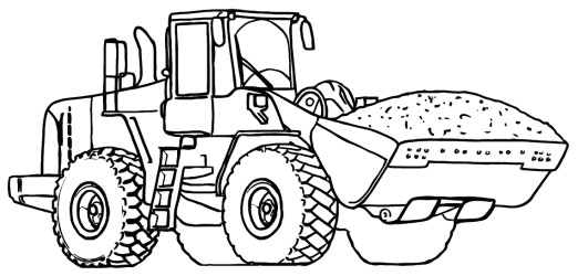
Figure 1 Fourteen-metric ton wheel loader used as a reference vehicle in this research.
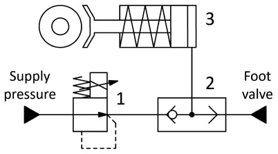
Figure 2 Modified prototype braking system allowing for TC implementation.
In order to assess the TC capabilities for real-world implementation, the machine prototype has been retrofit with an electro-hydraulic braking system allowing for independent control of the braking pressures at each wheel. As shown in Figure 2, an electrically-controlled pressure reducing valve (1) generates a certain pressure based on the TC system command. The shuttle valve (2) takes this pressure and the pressure commanded by the operator foot valve and allows the higher pressure to act on the wheel brake (3). In this way, TC schemes can be realized on the prototype, and their performances and the machine dynamic response can be compared to those found in simulation. More information can be found in [9].
4 Nonlinear Vehicle Model
In order to begin formulating the controller for this system, the dynamics of the vehicle itself must be described. For the purposes of designing a proper model-based nonlinear controller, it is of utmost importance that the modeling equations are as accurate to the real-world system as possible. A controller built on an inaccurate system model will not be able to efficiently track a desired trajectory.
The vehicle dynamics equation for this heavy-duty system were developed and validated in more detail in [8], but they are summarized here for further discussion. It should be noted that the controller will run separately on each wheel, so a quarter-car model (i.e. only incorporating the dynamics of one wheel) is sufficient for this work (see Figure 3).
The model begins simply with the linear and rotational equations of motion for the vehicle chassis and wheel, respectively.
| (1) |
| (2) |
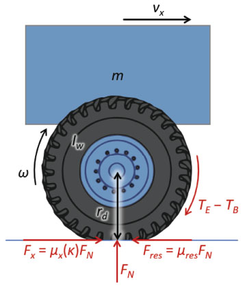
Figure 3 Driven wheel on flat ground surface.
In Equation (1), m is the mass supported by the wheel (typically roughly one quarter the mass of the total machine) and vx is the longitudinal velocity of the vehicle. The longitudinal pushing force at the wheel Fx and the resistive forces Fres (including rolling resistance and air resistance) are represented as friction coefficients (μx and μres) multiplied by the normal force at the wheel FN, which is allowed to vary with time. The resistive force always opposes the motion of the vehicle. The longitudinal friction force coefficient μx is a function of wheel slip ratio κ, which is a quantity comparing the rotational motion of a given wheel to the linear motion of the vehicle. The rotational dynamics in Equation (2) also include the wheel moment of inertia Iw, the rotational velocity of the wheel ω, the engine input torque to the wheel TE and braking torque TB, and the dynamic radius of the tire rd. It is already apparent that the system at hand contains significant nonlinearities. Both equations contain the function μx(κ), a relationship which for this work is represented using Pacejka’s Magic Formula Tire Model [20].
| (3) |
where Bx, Cx, Dx, and Ex are constants used to fit the model to experimental data. This equation is clearly nonlinear in κ, which below is shown to be a state for this system. Furthermore, Equation (1) contains the sgn function, which has a significant discontinuity at zero.
As described in [8], the wheel slip ratio κ has its own dynamics, making it a state for the system. Its dynamics are described as shown in Equation (4).
| (4) |
In this equation, B is the longitudinal relaxation length of the wheel, and all other variables are the same as above. Once again, the slip ratio dynamics contain yet another nonlinearity, this time in the form of an absolute value.
5 Sliding Mode Control Development
Due to the existence of these inherent system nonlinearities, it is clear that the best approach for controlling the wheel slip will include a nonlinear controller, as linear control methods cannot account for all of the complex system dynamics. Past work from the author’s research group has dealt with non-model-based linear controllers. For example, a PID controller was created with some additional logic meant to counteract negative system features such as integrator windup (see also [9]). Another controller was designed based on a linearized version of the system model shown in this work (that is, the system equations were linearized in real time and a linear control law was used). However, both of these options fail to capture the nonlinear dynamic information which can be leveraged to give the most accurate description of the machine behavior. Therefore, it is likely that the best control solution is one which can account for all the nonlinear features of the model described in Section 4.
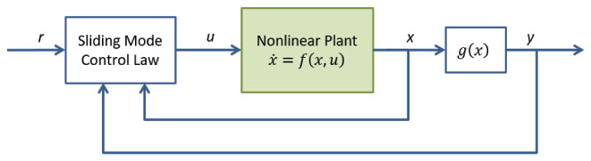
Figure 4 Sliding mode controller construction.
To that end, a sliding mode controller was developed which is capable of controlling the wheel slip for each individual wheel of the vehicle. Sliding mode is a nonlinear control concept capable of handling both disturbances and model parameter uncertainty [21]. In order to do that, it uses both an estimate of the system plant dynamics x and the measured output y (see Figure 4). Therefore, it is well-suited to controlling systems like off-road vehicles, where parameters can vary rapidly and widely. These uncertainties are discussed in more detail below.
5.1 Nonlinear State-Space Model
The first step in designing the sliding mode controller is to create a state-space model from the dynamic equations outlined in Section 4. There are three states (x1, x2, x3) to this system model: the longitudinal vehicle velocity vx, the wheel rotational velocity ω, and the wheel slip ratio κ. In this particular system architecture, the braking torque into the wheel TB is the only control action available to the system. Therefore, it is represented as the system command input u.
| (5) |
To generate the form of the controller, the system output must also be selected. It has been common to use wheel slip ratio κ as the system output for other TC schemes (cf. [9]). However, in real-world implementation, low vehicle velocities (wherein the reference machine typically operates) can cause numerical issues with slip ratio. Therefore, the prototype implementation uses simply the slip velocity vslip as the output to be controlled. At higher velocities, these two concepts are similar and have roughly the same behavior. However, at low velocities, the slip velocity is better behaved, especially for real-world applications. Therefore,
| (6) |
The controller set forth in this section will be designed according to this output definition. However, the basic methodology is the same for any arbitrary system output.
5.2 Feedback Linearization Control Law
The next step in the development of the controller is to develop the “Sliding Mode Control Law,” as shown in Figure 4. There is no single control law that is required for use with the sliding mode controller [22]. In this case, because the system at hand is nonlinear, a suitable nonlinear control law was chosen: feedback linearization (Figure 5). This control law attempts to cancel out the effect of nonlinearities in the system and then drive the error to zero using standard linear control systems approaches. It does this through use of a transformed state vector z.
Once the system output y has been chosen as was done in Equation (6) above, the next step is to determine the relative degree of the system. This is done by taking Lie derivatives of the output until a form is reached which contains the system input u. For this system, the first Lie derivative of the output is as follows.
| (7) |
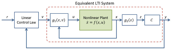
Figure 5 Feedback linearization control structure.
Because this derivative explicitly contains u, the relative degree of this system is r = 1. This means that the transformed system will have r = 1 external state variable and n − r = 3 − 1 = 2 internal state variables. The external state ξ is the output as previously defined.
| (8) |
As long as the internal states are stable (that is, the system is “internally stable”), the internal states simply need only be linearly independent of each other and of the external state. As they do not contain the input u, the internal states η1 and η2 were chosen as x1 and x3, respectively, so that no state is a linear combination of the others. That is,
| (9) |
Therefore, the transformed state vector becomes:
| (10) |
where g2(x) is the coordinate transformation operation from x to z. In order to create the equations for the control law, the external state dynamics are needed. They are the same as in Equation (7).
| (11) |
The dynamics can now be split into pure state and input dynamics.
| (12) |
where
| (13) |
| (14) |
The control law itself is based on a cancellation of the contributions from the nonlinear components in the model and the addition of a linear control signal v to drive the output error to zero.
| (15) |
Having arrived at this law, what remains is to generate an appropriate linear control law v to drive the error to zero. This is done using the following controller.
| (16) |
If a1 is chosen such that s + a1 is Hurwitz stable, then the controller itself is stable, and error e will go to zero with increasing time. Furthermore, the internal states r of this system are indeed stable, meaning that the overall controlled system is stable. Therefore, this feedback linearization controller is a suitable nonlinear controller for use as the sliding mode control law.
5.3 Determination of Uncertain Parameters
As sliding mode control is capable of handling uncertainties in the system model, the next task in developing the controller is to define which model parameters are uncertain and define boundaries within which they are allowed to vary. In general, there are two different reasons to create an uncertain parameter: if the parameter is difficult to measure accurately or if it can vary during operation. In vehicle systems, there are many such values, so an effort should be made to minimize the set of uncertain values.
For the system described in Equation (5), four uncertain parameters (θ1 through θ4) were identified. The first parameter chosen is the coefficient of resistance μres. This value is very difficult to measure, and it can vary widely from moment to moment. Second was the machine mass m. This value is relatively simple to measure, but for a load handling machine like a wheel loader, it can change very suddenly. Furthermore, the shifting weight distribution affects this value, as the controller is being constructed on a quarter-car model of the vehicle. The third uncertain parameter is the wheel relaxation length B. In most systems, this value can be considered constant (as long as the tires are well maintained), but it can be quite difficult to measure accurately. Finally, the engine torque into the wheel TE is also considered uncertain. For this particular system architecture, the engine torque cannot be controlled (as there is no direct access to the engine control unit), and therefore it is, in effect, a disturbance. By treating it as an uncertain parameter, the operator can command a wide range of different torques, and the controller will respond appropriately. Therefore, the vector of uncertain parameters for this system is as follows.
| (17) |
It should be noted that, while these terms are considered uncertain, the sliding mode controller requires them to vary within some defined region [23]. Each value θi is assigned a range of allowable values, and a representative estimate of that parameter is given. This then generates a parameter error , which is used in the formulation of the controller itself. The uncertain parameter limits for this particular work are covered by confidentiality and are not shown here, but they are based on reasonable values for the machine based on experimental data. Most often, the average of the maximum and minimum possible values for each parameter is used.
The new state-space model incorporating unknown terms is now defined as:
| (18) |
The uncertain terms from θ show up in all three equations. Therefore, it is important to bound the uncertainties properly, as failing to do so will severely impact the controller performance.
Despite the possible variability in both parameters, μx and μres cannot logically be treated in the same way. Whereas the resistive force coefficient μres is a relatively small term which may vary significantly within a fairly well-understood range, the longitudinal friction force coefficient μx is much larger and can be modeled reasonably well. By allowing μres to be an uncertain term, its small effect can be accounted for without requiring cumbersome sensing strategies. However, μx is a primary driver of the vehicle dynamics, and the controller must contain some logical model of that term to function well. Therefore, these two coefficients cannot simply by rolled into a single uncertain term.
5.4 Sliding Mode Control Law
The feedback linearization law presented above is suitable for conditions with perfect model matching; however, the introduction of uncertain parameters for the model calls for a modification to the control law. This controller is still built on the same transformed state vector z constructed in Section 5.2. However, it includes additional considerations for handling the uncertain terms. Therefore, the new external state dynamics of the system become:
| (19) |
In order to design the sliding mode control law, it is first necessary to define a target surface s(x) = 0 for the system error. Given that the system model and uncertainty bounds are accurate, the sliding mode controller will drive the system onto the sliding surface in a finite amount of time, and the system should remain on that surface [24]. For this system, the target surface and its time derivative were defined as follows.
| (20) |
| (21) |
The actual sliding mode control law is now formulated as:
| (22) |
where um is the model compensation component of the control and us is the sliding mode component. Each of these elements has a part to play in the proper control of this system. The model compensation component attempts to cancel out the dynamics of the nonlinear model. However, as uncertainties in the model are present, the parameter estimates must be used.
| (23) |
Using this model compensation control, the error dynamics are now shown to be:
Sliding mode control laws are by nature designed to switch between two levels, depending on the sign of s(t). For implementation in real-world systems, it is typically not practical to use a sgn function for such a switching condition, due to the fact that physical systems are not capable of immediate switching between two levels. Furthermore, such a stringent condition often results in actuator demands which are extremely high and/or out of bounds for the controller. Therefore, a saturation function is used instead.
| (24) |
In this equation, ψ is the so-called boundary thickness, which controls how quickly the saturation function varies from −1 to 1 as s changes. The implication of using a saturation function instead of sgn is that the stated previously performance of the controller is no longer guaranteed. A small amount of error will now be allowed by the controller. But the tradeoff for this decrease in performance is a controller which gives reasonable command values which can be implemented on a real-world system.
The function h(x, t) is chosen such that it is always greater than the effect of the estimation error in the system. That is,
| (25) |
The addition of constant h0 provides an added margin to the function, ensuring that the command us is always negative-definite (i.e. that it will drive the error to zero). Function h(x, t) can have many different formulations, provided that condition (25) is met. For this work, h(x, t) was chosen as a constant value greater than the maximum absolute error of the system.
6 Simulation Work
Once the nonlinear sliding mode controller was developed, it was tested in simulation to verify its ability to control wheel slip. The simulation case used here is the same as in previous work by the author’s research group [8]. As shown in Figure 6, this test condition involves the fourteen-metric ton machine approaching large tires which are placed against a barrier. The model contains information about vehicle engine torque and describes how its weight is transferred between the two axles in a dynamic condition, taking into account both vehicle acceleration and external loading. It should also be mentioned that the parameter estimates used for the sliding mode controller for all parameters in Equation (17) are different from their actual values in the simulation model (varying from the actual values by 5–10%). This was done intentionally to assess the controller performance in the face of uncertainties.
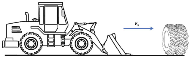
Figure 6 Test condition for TC simulation.
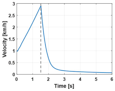
Figure 7 Simulated vehicle linear velocity.
At the beginning of the simulation, a constant input torque is given to the driveshaft of the wheel loader, which causes the machine to accelerate forward into the barrier. The tires on the barrier generate a resistive force Fpush, which is modeled as a spring-damper force opposing the motion of the wheel loader. As the vehicle impacts the tires, the resistive force increases, eventually causing the vehicle to slow down (Figure 7) and the wheels to slip against the road surface. As the wheels begin to slip, the TC system brakes the spinning wheels according to the sliding mode control law developed in Section 5. This provides an assessment of how well the controller can control wheel slip. The pushing force at once the vehicle impacts the tires against the barrier is modeled as a unilateral spring-damper system, as shown in [8].
The controller results of this simulation are shown in Figure 8. This plot shows the slip velocity of a wheel on the vehicle, which is the process variable being controlled by the TC system. The plot has been normalized with respect to the controller’s slip velocity setpoint, to show the relative performance of the controller. In this simulation, the vehicle impacts the tires on the barrier at around time t = 1.2 seconds. At that moment, the wheel begins to slip more aggressively against the ground. As that happens, the TC system activates the brakes, and brings the wheel slip back under control.
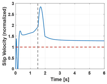
Figure 8 Simulated wheel slip velocity (sliding mode control).
Figure 8 demonstrates some important aspects of the sliding mode control. First, within the first 0.3 seconds of the simulation, the wheel slip crosses above the setpoint, and the controller acts quickly to correct it. This overcorrection occurs during acceleration, and it could represent an issue if it impacts the operator perception. However, once the vehicle impacts the tires, the sliding mode control acts very quickly (correcting the slip within a few tenths of a second) and without any sort of overshoot. Finally, it should be noted that the controller does not achieve zero tracking error, even in steady state.
As was mentioned in Section 5, the saturation function used in lieu of the sgn function causes a relaxation of the controller’s ability to drive the error to zero. Depending on the controller design and parameters (such as boundary thickness ψ), this steady-state error can be reduced somewhat. It is up to the system designers to determine what an acceptable error is for the system. This performance was deemed sufficient for the investigation at hand. Furthermore, this performance was achieved even with inaccurate parameter estimates in the controller model. Better parameter estimate values will result in even better controller performance, but there will always be some amount of error in real-world operation.
The sliding mode controller shows significant improvement over the non-model-based linear control approach (based on a PID control law) which has been used in the past. For comparison, the results of that linear controller under the same operating conditions are shown in Figure 9. The sliding mode control performs markedly better, especially at the very beginning of the simulation, wherein the linear controller allows slip velocities up to five times the setpoint value before the traction control is able to act and correct it. After impacting the tires, the linear controller performs approximately as well as the sliding mode controller, with a peak only reaching about two times the setpoint. However, the response also contains significant oscillations which slow down the settling time compared to the sliding mode control. These results indicate that, even with inaccurate parameter estimates, the sliding mode control is able to act more quickly than the PID-type control. This is the advantage of compensating for system behavior by using a model-based control scheme [25]. The non-model-based linear controller can only respond to the error and its dynamics; however, the sliding mode control responds appropriately according to how the system will react to the control action.
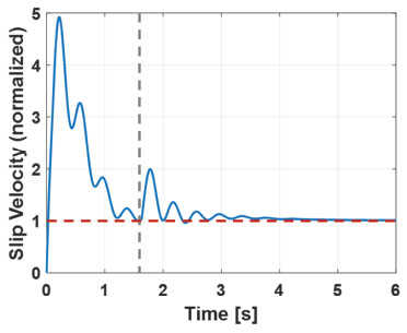
Figure 9 Simulated wheel slip velocity (PID control).
7 Experimental Validation
The TC scheme using sliding mode control was then implemented on a fourteen-metric ton prototype wheel loader and tested in controlled laboratory tests. The experimental setup for these tests is shown in Figure 10. Much like the simulation condition of Section 6, the experimental setup includes a barrier with tires against it to cushion the impact of the vehicle. Steel plates were also used on the ground to give the wheels a ground condition which had less friction than concrete but was still very repeatable.

Figure 10 Setup for experimental testing.
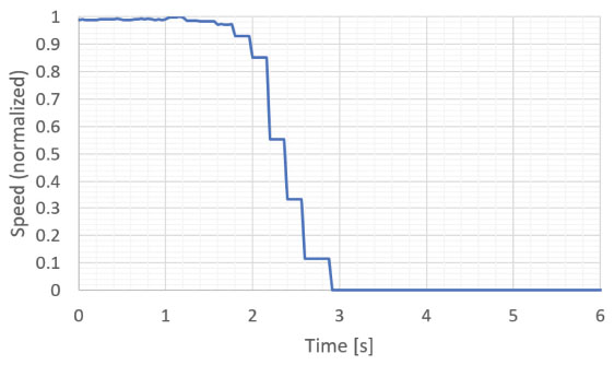
Figure 11 Representative speed profile for wheel loader during laboratory testing.
Again, like the simulated test condition, the experimental tests involved the reference machine driving up to the barrier and impacting the tires. Once the vehicle made contact with the tires, the throttle was increased to cause the wheels to slip against the steel plates. A vehicle speed measurement from a representative test is shown in Figure 11. As the vehicle came to a stop, the TC then acted to slow down the wheels which were slipping.
Measurements were made with several different sensors installed on the wheel loader. The complete sensor setup for the system is shown in Figure 12. Wheel speeds were measured to calculate wheel slip for creating the TC signals to each brake. The implement positions and working pressures were also measured. By solving a static force balance treating the implement as a loaded structure, the resistive force generated by the barrier can be calculated. More information on this methodology can be found in [17]. Using these measurements, the performance of the controller was assessed.
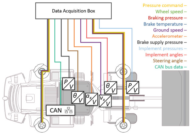
Figure 12 Instrumentation setup for experimental wheel loader testing.
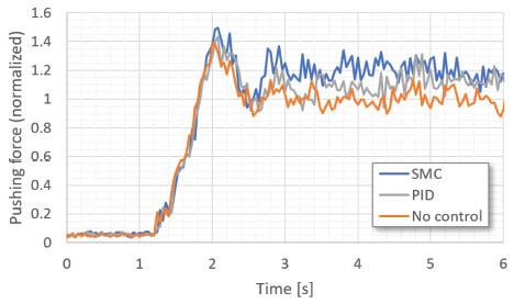
Figure 13 Experimental pushing force results with sliding model control implemented.
The data from three different tests is shown in Figure 13, one test with the stock machine and no TC active (“No control”), one with the previously-used linear control (“PID”), and one test with the sliding mode control (“SMC”). The data has been arranged so that the vehicle impacts the tires at around time t = 1 second. Furthermore, the data was also normalized with respect to the average pushing force of the uncontrolled machine after impacting the tires. All three tests exhibit the same behavior at first, with a relatively large initial impact force which then decreases as the wheels begin to slip against the steel plates.
However, at this point, the TC systems activate and brake the wheels significantly. As the vehicle pushes against the tires, the spinning wheels of the uncontrolled machine are never able to regain any of the lost pushing force. On the other hand, the system with TC is able to achieve a significantly higher pushing force, quickly recovering the majority of the force lost when the wheels began to slip. In fact, the sliding mode control acts rapidly enough that the pushing force for the controlled system never dips quite as low as the uncontrolled case, and its force is consistently higher for the duration of the test. The PID control also shows better pushing force results than the uncontrolled case; however, it is clear that the sliding mode control achieves higher forces than the PID control for the first few seconds after impacting the barrier.
In order to assess the overall performance of the controller, multiple repetitions of tests with each control structure were run. Objective functions were generated to compare the systems in an objective way. The first objective function, slip distance, is simply a time integral of wheel slip velocities. The second is the time average of the pushing force for the system. Both are taken within a short time window (of a few seconds) after the vehicle impacts the tires, similar to the length of time in which an operator would dig into a material pile with a wheel loader [26]. This means that controllers which act to reduce tire slip more quickly will achieve better results. The operating cycles for wheel loaders are often time-sensitive, so it is important that the system be able to correct for wheel slip quickly. The results from these tests are shown in Figure 14.
From this figure, it is apparent that the sliding mode control performs quite well. Both sliding mode and the previously-implemented PID control are capable of reducing wheel slip and increasing pushing force. However, the sliding mode control outperforms the linear control in both cases. For slip distance (Figure 14(a)), the linear control shows a reduction of 34%, whereas sliding mode control reduces the wheel slip by 54%. Average pushing force (Figure 14(b)) does not show quite as drastic a change. Nevertheless, the linear control and sliding mode control were able to increase the average pushing force by 10% and 19%, respectively. This will likely translate into more machine productivity, in terms of faster digging times and more material removed per cycle. The standard deviation within each data set is approximately 6.5% of the uncontrolled force value. Therefore, further work may be needed to establish the statistical significance of this data. However, for a first result, it is very promising.
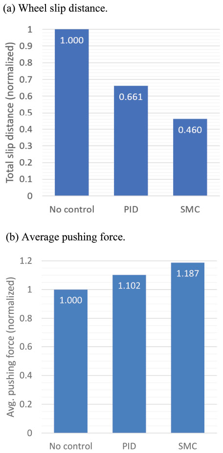
Figure 14 Comparison of sliding mode control (SMC) with baseline (No control) and linear controller (PID) performance.
8 Conclusions
This work focuses on the development of a nonlinear control law for active TC of heavy-duty machines using independent braking. Using a wheel loader as a reference case, a nonlinear vehicle model was described. Then this model was leveraged in order to develop a controller which would be suitable for the system based on the machine dynamics. This was done through the formulation of a sliding mode control structure using a feedback linearization-type coordinate transformation. The sliding mode approach allows for parameter uncertainties; therefore, four different parameters were identified which were allowed to vary within a certain regime. Finally, the sliding mode control law itself was constructed.
The sliding mode control was tested first in a simulation based on the vehicle dynamics equations. As the TC showed positive results in simulation, it was then implemented on a real-world prototype which had been modified to allow for independent braking. Tests were conducted using the original system and the TC system using sliding mode control. The results of these tests were also compared with a previously-designed non-model-based linear controller. In comparison, the sliding mode control shows a significant improvement in controlling wheel slip, even reducing it by 30% compared to the linear control. It also increases average pushing force by 9% above the uncontrolled case, which is marginally better than the linear control. This represents a marked advancement in traction control development for off-road construction machines.
References
[1] S. M. Savaresi and M. Tanelli, Active Braking Control Systems Design for Vehicles. London: Springer London, 2010.
[2] Y. B. Kim, J. Ha, H. Kang, P. Y. Kim, J. Park, and F. C. Park, “Dynamically Optimal Trajectories for Earthmoving Excavators,” Automation in Construction, vol. 35, pp. 568–578, Nov. 2013.
[3] T. D. Gillespie, Fundamentals of Vehicle Dynamics. Warrendale, PA: Society of Automotive Engineers, 1992.
[4] R. Rajamani, Vehicle Dynamics and Control, 2nd ed. New York, NY: Springer, 2012.
[5] R. N. Jazar, Vehicle Dynamics: Theory and Application, 2nd ed. New York: Springer, 2014.
[6] J. Y. Wong, Theory of Ground Vehicles, 4th ed. Hoboken, N.J: Wiley, 2008.
[7] A. F. Andreev, V. I. Kabanau, and V. V. Vantsevich, Driveline Systems of Ground Vehicles: Theory and Design. Boca Raton: CRC Press, 2010.
[8] A. Alexander and A. Vacca, “Longitudinal Vehicle Dynamics Model for Construction Machines with Experimental Validation,” IJAME, vol. 14, no. 4, pp. 4616–4633, Dec. 2017.
[9] A. Alexander and A. Vacca, “Real-Time Parameter Setpoint Optimization for Electro-Hydraulic Traction Control Systems,” in Proceedings of 15th Scandinavian International Conference on Fluid Power, Linköping, Sweden, 2017, pp. 104–114.
[10] S. Kuntanapreeda, “Traction Control of Electric Vehicles Using Sliding-Mode Controller with Tractive Force Observer,” International Journal of Vehicular Technology, vol. 2014, pp. 1–9, 2014.
[11] J. Li, Z. Song, Z. Shuai, L. Xu, and M. Ouyang, “Wheel Slip Control Using Sliding-Mode Technique and Maximum Transmissible Torque Estimation,” Journal of Dynamic Systems, Measurement, and Control, vol. 137, no. 11, p. 111010, Aug. 2015.
[12] J. van der Burg, A. Kheddar, and P. Blazevic, “Terrain-Adaptive Traction Control System for Intelligent All-Terrain Vehicles,” IFAC Proceedings Volumes, vol. 31, no. 3, pp. 57–62, Mar. 1998.
[13] H. Lee and M. Tomizuka, “Adaptive Vehicle Traction Force Control for Intelligent Vehicle Highway Systems (IVHSs),” IEEE Transactions on Industrial Electronics, vol. 50, no. 1, pp. 37–47, Feb. 2003.
[14] M. Schreiber and H. D. Kutzbach, “Influence of Soil and Tire Parameters on Traction,” Research in Agricultural Engineering, vol. 54, no. 2, pp. 43–49, 2008.
[15] P. V. Osinenko, M. Geissler, and T. Herlitzius, “A Method of Optimal Traction Control for Farm Tractors with Feedback of Drive Torque,” Biosystems Engineering, vol. 129, pp. 20–33, Jan. 2015.
[16] P. Osinenko and S. Streif, “Optimal Traction Control for Heavy-duty Vehicles,” Control Engineering Practice, vol. 69, pp. 99–111, Dec. 2017.
[17] A. Alexander, A. Sciancalepore, and A. Vacca, “Online Controller Set-point Optimization for Traction Control Systems Applied to Construction Machinery,” in Proceedings of the 2018 Bath/ASME Symposium on Fluid Power and Motion Control, Bath, UK, 2018.
[18] H. B. Pacejka and I. Besselink, Tire and Vehicle Dynamics, 3rd ed. Amsterdam: Elsevier/Butterworth-Heinemann, 2012.
[19] S. K. Mohan and R. C. Williams, “A Survey of 4WD Traction Control Systems and Strategies,” 1995.
[20] H. B. Pacejka and E. Bakker, “The Magic Formula Tyre Model,” Vehicle System Dynamics, vol. 21, no. S1, pp. 1–18, Jan. 1992.
[21] W. S. Levine, Ed., The Control Handbook, 2nd ed. Boca Raton, Fla.: CRC Press, 2011.
[22] R. Husson, Ed., Control Methods for Electrical Machines. London: Hoboken, NJ: ISTE; John Wiley, 2009.
[23] H. K. Khalil, Nonlinear Systems, 3rd ed. Upper Saddle River, NJ: Prentice Hall, 2002.
[24] L. Wu, P. Shi, and X. Su, Sliding Mode Control of Uncertain Parameter-Switching Hybrid Systems. Chichester, West Sussex, United Kingdom: John Wiley & Sons, Inc, 2014.
[25] L. C. Westphal, Handbook of Control Systems Engineering. Boston, MA: Springer US, 2001.
[26] M. D. Worley and V. La Saponara, “A Simplified Dynamic Model for Front-end Loader Design,” Proceedings of the Institution of Mechanical Engineers, Part C: Journal of Mechanical Engineering Science, vol. 222, no. 11, pp. 2231–2249, Nov. 2008.
Biographies

Addison Alexander received a B.S. in Mechanical Engineering from the University of Kentucky in 2013 and an M.S. and Ph.D. in Mechanical Engineering from Purdue University in 2016 and 2018, respectively. His Ph.D. work was done at the Maha Fluid Power Research Center at Purdue University, focusing on advanced control of mobile hydraulic machinery.

Andrea Vacca is a Professor of Fluid Power System and he currently leads the Maha Fluid Power Research Center of Purdue University, USA. Goals of his research are the improvement of energy efficiency and controllability of fluid power machines and the reduction of noise emissions of fluid power components.
International Journal of Fluid Power, Vol. 20_3, 375–400.
doi: 10.13052/ijfp1439-9776.2035
© 2020 River Publishers