Two-Dimensional Projection Based Wireless Intrusion Classification Using Lightweight EfficientNet
Hailyie Tekleselassie
School of Informatics, Wolaita Sodo University, Wolaita sodo, Ethiopia
Department of Information Systems, Addis 3Ababa, Ethiopia
E-mail: hailyie.tekleselase@wsu.edu.et
Received 07 January 2022; Accepted 05 May 2022; Publication 07 November 2022
Abstract
Internet of Things (IoT) networks leverage wireless communication protocol, which adversaries can exploit. Impersonation attacks, injection attacks, and flooding are several examples of different attacks existing in Wi-Fi networks. Intrusion Detection System (IDS) became one solution to distinguish those attacks from benign traffic. Deep learning techniques have been intensively utilized to classify the attacks. However, the main issue of utilizing deep learning models is projecting the data, notably tabular data, into image-based data. This study proposes a novel projection from wireless network attacks data into grid-like data for feeding one of the Convolutional Neural Network (CNN) models, EfficientNet. We define the particular sequence of placing the attribute values in a matrix that would be captured as an image. By combining the most important subset of attributes and EfficientNet, we aim for an accurate and lightweight IDS module deployed in IoT networks. We examine the proposed model using the Wi-Fi attacks dataset, called AWID dataset. We achieve the best performance by a 99.91% F1 score and 0.11% false positive rate. In addition, our proposed model achieved comparable results with other statistical machine learning models, which shows that our proposed model successfully exploited the spatial information of tabular data to maintain detection accuracy. We also successfully maintain the false positive rate of about 0.11%. We also compared the proposed model with other machine learning models, and it is shown that our proposed model achieved comparable results with the other three models. We believe the spatial information must be considered by projecting the tabular data into grid-like data.
Keywords: Intrusion detection, impersonation attack, convolutional neural network, anomaly detection..
1 Introduction
Nowadays, the Internet of Things (IoT) has developed very rapidly. The Internet has become a primary need for everyone. People are always connected to the Internet network through their smartphone, laptop, or personal computer. Adults and kids, and older people are inseparable from their devices. The recent technology development of IoT networks has led to the prosperity of smart environments [1]. Information pooled by IoT sensors could manage smart city applications’ assets, revenues, and resources with increased performance and efficiency [2].
IoT is commonly applied in particular domains such as smart grids, smart cities, and smart homes [3]. Jalal et al. provided the one advantage of using smart homes for helping daily human life [4]. At the same time, Asaad et al. reviewed the benefit of leveraging smart grids in a country [5]. Despite all the prosperity, IoT networks leave a vulnerable hole to be exploited by adversaries, which is the use of wireless communication channels [1]. When people are connected to the Internet network, they are vulnerable to various malicious cyber attacks from adversaries. Different types of attacks on WiFi include impersonation attacks, injection attacks, and flooding [6].
An impersonation attack is a form of attack in which an adversary poses as a trusted person to trick the victim [7]. Usually, the adversary will collect someone’s data through the Internet and use it to convince the victim that he is the real person. An injection attack is a malicious code injected into the network and steals all the data from victims’ databases [8]. Several well-known injection attacks are SQL Injection, Cross-Site Scripting (XSS), and SMTP/IMAP Command Injection. Finally, a flooding attack is when adversaries send massive traffic into the victim’s network [9]. The main goal is to create network congestion to hinder legitimate traffic. Because of these various attacks, a defensive mechanism as a countermeasure is needed. The mechanism is called Intrusion Detection System (IDS).
IDS can be classified into two classes: signature-based and anomaly-based IDS [10, 11]. Signature-based IDS is a classic IDS system that uses an attack signature database as the detection tool. Anomaly-based IDS monitors the inbound traffic to detect any malicious action. However, there is a problem with the current IDS. Recent publications of IDS show that it is difficult to handle complex datasets with high dimensionality [12]. Because of that reason, we want to propose a lightweight machine learning framework using two-dimensional projection for IDS. We train our system using the AWID2 dataset, an impersonation attack dataset that consists of four classes: normal, impersonation, injection, and flooding.
This paper proposes a two-dimensional projection-based IDS system that utilizes lightweight EfficientNet for the classification process. Our system consists of three main parts: 1. Dataset Preparation, 2. Data Preprocessing with feature selection using Random Forest, and 3. Image Classification using EfficientNet. This paper is the first DL-based IDS that combines data-to-images projection with EfficientNet for IDS to the best of our knowledge. Compared to previous works, our main contributions are listed below:
1. We provide a data-to-image conversion process by using a zigzag scan pattern from the JPEG images compression technique based on their feature importance.
2. We handle the IDS data conversion into graphical number format that represents the attribute value of each feature.
3. Our framework explores feature selection using random forest models with cross-validation.
4. We propose a lightweight CNN-based IDS using EfficientNet-B0 architecture to handle complex datasets [13].
5. Our proposed system identifies the spatial correlation between features through grid-like images.
6. We provide the performance analysis by highlighting our model’s F1 score and accuracy.
The remainder of this paper is organized as follows: Section 2 provides related work on utilizing deep learning techniques in IDS. The proposed model and data processing are explained in Section 3. Section 4 shows the experimental results of each module in the proposed model. While Section 5 provides the comparison of the proposed model with other machine learning models. Section 6 closes this paper with conclusions and outlines future research directions.
2 Related Works
Study about IDS has been conducted continuously since several years ago. Starting from using a list of attack databases; until leveraging the latest machine learning method. Smys et al. proposed a hybrid convolutional neural network model for IDS suitable for a wide range of IoT applications [14]. Khan et al. introduced an efficient and intelligent IDS to detect malicious attacks [15]. They leverage Convolutional Autoencoder (Conv-AE) from spark MLlib for misuse attack detection. Another work by Li et al. introduced an AE-based IDS on random forest feature selection [16]. However, these works face difficulty in handling the traffic of massive IDS datasets.
SwiftIDS tried to address the scalability issue by using a parallel intrusion detection mechanism to analyze the network traffic [17]. The system’s performance showed an encouraging performance, but it still requires a longer processing time. Another approach by Rahman et al. improved the parallel IDS model by applying side-by-side feature selection, followed by a single multilayer perceptron classification [18]. Finally, a hybrid scheme that combines the deep Stacked Autoencoder (SAE) and machine learning methods is introduced by Mighan et al. [19]. Those works show a relation between a number of features, processing time, and accuracy, which are three main variables in the IDS model.
3 Methodology
Our methodology in this study is divided into 4 main parts, namely data preparation, data preprocessing, modeling, and evaluation. In data preparation we used several techniques to obtain train, validation, and test sets. Tabular data was converted into image data through data preprocessing. Then we did the modeling to classify the image data. Finally, we evaluated the performance of the trained model. You may select up to 8 categorical data columns for stratification. The strata will be created as the combination of all unique values in the stratification columns. For example, if stratification column 1 has three unique values (A, B, and C) and stratification column 2 has two unique values (1 and 2), then the six resulting strata would be A1, A2, B1, B2, C1, and C2. Random samples are generated independently within each stratum. Any rows for which any of the stratification values are missing will not be eligible for sampling. The number of items sampled from each stratum is controlled by the Sample Allocation among Strata and Sample Size options. In the example below, S1 (with values A, B, and C) is entered as the stratification column. There are twice as many A’s as B’s and C’s. Since the sample allocation among strata is proportional to sample size, there are twice as many values selected from stratum A than from B and C.
3.1 Data Preparation
We used the normalized AWID2 dataset, this dataset has a Test and Train sets. We combined these 2 parts into a dataset to avoid bias, then from this dataset we created train, validation, and test sets. The entire data preparation process can be seen in Figure 1 below.
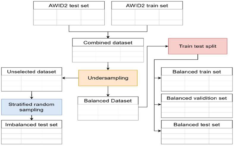
Figure 1 Data preparation process.
Our combined dataset has 2,371,218 samples with 154 columns plus 1 target column. In this dataset there is 1 normal (0) class and 3 attack classes, that is impersonation (1), injection (2), and flooding (3). More than 90% of the existing samples are normal (0) class, this causes an imbalanced class distribution.
We used an undersampling technique to tackle imbalances in our dataset and to reduce the number of samples used in order to save resource consumption. We used 40,000 samples or 1.7% of total samples with 10,000 samples per class. From this process we got a new dataset, the Balanced Dataset.
We divided our balanced dataset into train, validation, and test sets with a ratio of 8:1:1, we got 32,000, 4,000, and 4,000 data for train, validation and test, sequentially. We also created an imbalance test set that has the same distribution as our combined dataset. In this test set, 20,000 samples are used with the distribution as shown in Figure 2. In total, we got a test set with the size of 24,000 samples or 1% from our combined dataset.
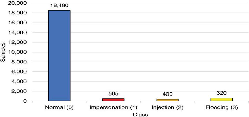
Figure 2 Imbalanced test set distribution.
3.2 Data Preprocessing
The method we used is data-to-images projection by writing feature values on an image using a program. Each data instance is turned into a single image. The writing of this feature value follows a pattern where each value fills 1 grid. The number of grids in one image is the square of positive integers so that we get n n grids. Due to the nature of the method, we didn’t use all features in the data. Therefore, the first step in our method is to perform feature selection.
In feature selection, we sorted the features based on their importance in influencing the classification. From this ranking we took the top-k features, where k is the number of features to be used. Ranking was obtained through the average value of feature importance from 5 random forest models. We trained 5 random forest models using 5-cross-validation from our train set. This whole process can be seen in Figure 3.

Figure 3 Data preprocessing process.
The pattern we used in our method mimics the zigzag scan pattern in JPEG compression technique [13], as shown in Figure 4. The rank 1 feature is on the grid in the upper left corner, then the next feature follows a zigzag pattern so that the position of each feature based on its rank will look like Figure 4. The lowest rank feature is in the lower-right corner.
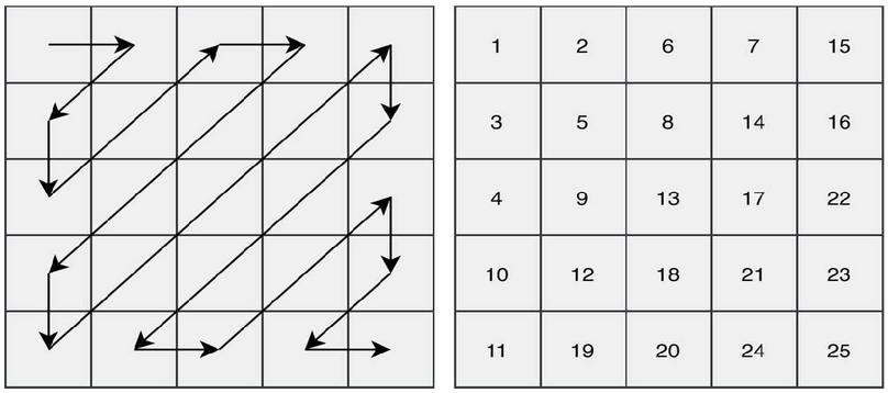
Figure 4 Pattern example for k 25 (left) and features placement based on their ranking (right).
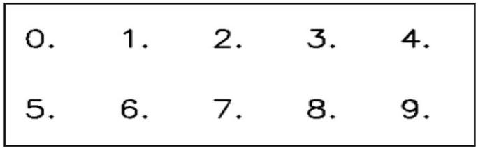
Figure 5 Numeric samples from Hersyler Simplex font.
The image we produced has a resolution of 224 224 with RGB channels for the entire k values. We wrote the feature value using the Hersley Simplex font with white color on an image with a black background. A sample of the Hersley font can be seen in Figure 5. To maintain consistency, we wrote each feature value in 3 decimal formats. The whole process of data-to-image projection was done using Python and OpenCV.
3.3 Image Classification
In this method, we used the Convolutional Neural Network model to classify the images we generated. We used the EfficientNet-B0 architecture [22], a light-weighted CNN model, which performed well on the ImageNet dataset while maintaining model efficiency. The nature of this architecture is suitable for application in low-end devices, which are preferred for use in wireless networks.
For our generated image that has 224 224 resolution with RGB channel, EfficientNet-B0 offered 4,054,695 total parameters or 16 MB file size in H5 format. This number is the smallest compared to other architectures in the EfficientNet family. We used the Tensorflow Framework running on an RTX 2070 laptop with 32 GB memory for our modeling purpose.
We trained our model for 10 epochs using a Stochastic Gradient Descent (SGD) as optimization algorithm with a learning rate 0.05 and a batch size of 32. We rescaled the pixel value so that it is in the range 0 to 1. There were 3 models that were trained on each k value, so there were 33 models that we trained. We did this to get more robust data from each image classification on value k. As a reminder, we trained each model on 32,000 images and 4,000 images as validation set.
4 Evaluation
4.1 Evaluation Metrics
For model evaluation, we used accuracy and F1. The accuracy score is good to see how well our model guesses the class, but it fails to provide good insight for the imbalanced dataset. So, for our imbalanced dataset, we used F1 score for our primary metrics. It combines precision and recall scores, making F1 scores provide better insight into how well our model predicts in imbalanced datasets. In our dataset there are 4 classes that make the task we did is multiclass classification. Precision, recall, and F1 score were originally matrices for binary classification, so we used weighted scores on precision, recall, and F1 scores for our multiclass classification.
From a different perspective, our classification can be seen as a binary classification. In this classification, the positive class (P) indicates the attack class (impersonation, injection, and flooding) and the negative class (N) indicates the normal class. This means True Positive (TP) will indicate the number of attack classes that have been detected correctly, False Negative (FN) indicates the number of attack classes that were not detected, False Positive (FP) indicates the number of normal classes detected as attack classes (False Alarm), and True Negative (TN) indicates the normal class that has been recognized correctly. Conversion from multiclass confusion matrix to binary confusion matrix can be seen in Figure 6.

Figure 6 Confusion matrix for multiclass to binary classification.
4.2 Feature Selection
As we mentioned before, we used feature ranking to decide the feature that we were putting for image projection. The complete list of our feature ranking can be seen in Table 1. The total of all feature importance scores is 1. The maximum importance score is 0.0708 belonging to feature 141. About 43% of features have an importance score close to zero. A score close to zero means some features may be just noises.
We plotted a graph of cumulative feature importance score, see Figure 7. We got a cumulative score of 1 using only 88 features, this confirms that the remaining 66 features are probably just noises. Based on this ranking, we get the top-k feature to be used on image projection. We used the value of k 25 as the baseline and we decreased and increased the value. In total we used 11 values of k, which was 4, 9, 16, 25, 36, 49, 64, 81, 100, 121, and 144.
Table 1 Feature rank
| Rank | Feature | Rank | Feature | Rank | Feature | Rank | Feature | Rank | Feature | Rank | Feature |
| 1 | 141 | 31 | 106 | 61 | 71 | 91 | 30 | 121 | 134 | 151 | 57 |
| 2 | 67 | 32 | 118 | 62 | 99 | 92 | 31 | 122 | 152 | 152 | 58 |
| 3 | 66 | 33 | 97 | 63 | 95 | 93 | 32 | 123 | 130 | 153 | 59 |
| 4 | 8 | 34 | 89 | 64 | 90 | 94 | 33 | 124 | 82 | 154 | 0 |
| 5 | 63 | 35 | 137 | 65 | 101 | 95 | 34 | 125 | 83 | ||
| 6 | 7 | 36 | 144 | 66 | 102 | 96 | 35 | 126 | 84 | ||
| 7 | 74 | 37 | 119 | 67 | 96 | 97 | 27 | 127 | 85 | ||
| 8 | 153 | 38 | 145 | 68 | 91 | 98 | 26 | 128 | 86 | ||
| 9 | 78 | 39 | 107 | 69 | 110 | 99 | 150 | 129 | 87 | ||
| 10 | 65 | 40 | 117 | 70 | 105 | 100 | 23 | 130 | 104 | ||
| 11 | 46 | 41 | 121 | 71 | 47 | 101 | 22 | 131 | 112 | ||
| 12 | 75 | 42 | 138 | 72 | 124 | 102 | 148 | 132 | 113 | ||
| 13 | 77 | 43 | 80 | 73 | 122 | 103 | 147 | 133 | 114 | ||
| 14 | 72 | 44 | 93 | 74 | 51 | 104 | 146 | 134 | 115 | ||
| 15 | 109 | 45 | 103 | 75 | 42 | 105 | 9 | 135 | 116 | ||
| 16 | 139 | 46 | 92 | 76 | 15 | 106 | 10 | 136 | 73 | ||
| 17 | 3 | 47 | 126 | 77 | 88 | 107 | 11 | 137 | 135 | ||
| 18 | 37 | 48 | 127 | 78 | 61 | 108 | 36 | 138 | 136 | ||
| 19 | 49 | 49 | 125 | 79 | 17 | 109 | 16 | 139 | 52 | ||
| 20 | 6 | 50 | 129 | 80 | 28 | 110 | 149 | 140 | 40 | ||
| 21 | 81 | 51 | 140 | 81 | 123 | 111 | 151 | 141 | 41 | ||
| 22 | 50 | 52 | 128 | 82 | 131 | 112 | 18 | 142 | 43 | ||
| 23 | 4 | 53 | 142 | 83 | 25 | 113 | 2 | 143 | 44 | ||
| 24 | 5 | 54 | 111 | 84 | 14 | 114 | 1 | 144 | 45 | ||
| 25 | 76 | 55 | 143 | 85 | 19 | 115 | 20 | 145 | 48 | ||
| 26 | 79 | 56 | 120 | 86 | 13 | 116 | 21 | 146 | 53 | ||
| 27 | 60 | 57 | 100 | 87 | 133 | 117 | 12 | 147 | 62 | ||
| 28 | 69 | 58 | 98 | 88 | 132 | 118 | 64 | 148 | 54 | ||
| 29 | 70 | 59 | 108 | 89 | 29 | 119 | 38 | 149 | 55 | ||
| 30 | 68 | 60 | 94 | 90 | 24 | 120 | 39 | 150 | 56 |
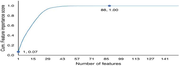
Figure 7 Cumulative feature importance score.
4.3 Image Projection Result
A sample of the images for each value of k that we used can be seen in Figure 8. It is important to mention that because we used the same resolution for each value of k, there were drawbacks in the feature writing. First, the writing of the feature value becomes smaller every time the value of k increases. Second, the writing of feature values deformed every time the value of k increases, as shown in Figure 9. This was happened because the number of pixels on each grid decreases as the value of k increases. The writing of the features value started to be hard to read at k 49, at k 144 the writing is only shaped like a straight line.
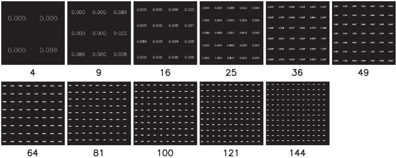
Figure 8 Image projection samples for each value of k.
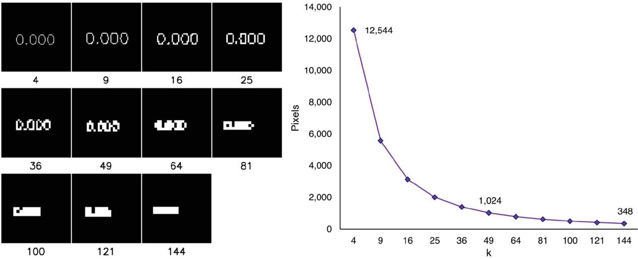
Figure 9 Writing in a grid for each value of k (left) and number of pixels per grid (right).
4.4 Test Result
Our experiment consists of the training of 3 models based on given top-k features ranking. We did 2 tests on our models, first was on a balanced dataset and second was on an imbalanced dataset. We compared our models using predefined metrics and we took the average score for each value of k (3 models for each value of k). The result of our test can be seen in Table 2.
We highlight the highest value in each column in the table. The model that uses 49 features looks better on the balanced dataset, while the model that uses 36 features looks better on the imbalanced dataset. F1 value and accuracy start to decrease at k 100. We argue that the range of k values that produce the best performance is from 25 to 100.
From this result, we see a decrease in performance in the imbalanced dataset compared to the balanced dataset. Although we cannot mention the significance of the decrease in performance, we assumed that this decrease was due to the larger number of samples in the imbalanced dataset. This may happen because we only use 1% of the dataset which may not be able to capture all the information in the imbalanced dataset. I usually use 5-fold cross validation. This means that 20% of the data is used for testing, this is usually pretty accurate. However, if your dataset size increases dramatically, like if you have over 100,000 instances, it can be seen that a 10-fold cross validation would lead in folds of 10,000 instances.
Table 2 Test result
| Balanced | Imbalanced | |||
| k | F1 Score | Accuracy | F1 Score | Accuracy |
| 4 | 96.73% 0.18% | 96.75% 0.18% | 92.70% 0.29% | 89.40% 0.46% |
| 9 | 98.18% 0.01% | 98.18% 0.01% | 99.52% 0.00% | 99.53% 0.00% |
| 16 | 98.60% 0.48% | 98.60% 0.48% | 98.17% 2.19% | 97.48% 3.17% |
| 25 | 99.91% 0.01% | 99.91% 0.01% | 99.89% 0.01% | 99.89% 0.01% |
| 36 | 99.92% 0.00% | 99.93% 0.00% | 99.91% 0.02% | 99.91% 0.02% |
| 49 | 99.94% 0.01% | 99.94% 0.01% | 99.88% 0.03% | 99.88% 0.03% |
| 64 | 99.94% 0.01% | 99.94% 0.01% | 99.89% 0.02% | 99.89% 0.02% |
| 81 | 99.93% 0.01% | 99.93% 0.01% | 99.90% 0.03% | 99.90% 0.03% |
| 100 | 99.93% 0.01% | 99.93% 0.01% | 99.89% 0.02% | 99.89% 0.02% |
| 121 | 99.84% 0.01% | 99.84% 0.01% | 99.58% 0.07% | 99.57% 0.07% |
| 144 | 99.53% 0.04% | 99.53% 0.04% | 98.96% 0.19% | 98.90% 0.21% |
4.5 False Alarm Rate and False Negative Rate
We plotted False Alarm Rate (FAR) and False Negative Rate (FNR) for each value of k, see Figure 10. We obtained these values by calculating the mean of the combined test results from the balanced and imbalanced dataset in a binary perspective, as we previously mentioned. The highest values of FAR and FNR were 11.50% at k 4 and 2.43% at k 9, sequentially. Configurations at k 25 have poor values, either FAR, FNR, or both. Meanwhile the FAR value starts to increase at k 100. These results strengthen our statement that the range of k values that produce the best performance is from 25 to 100.
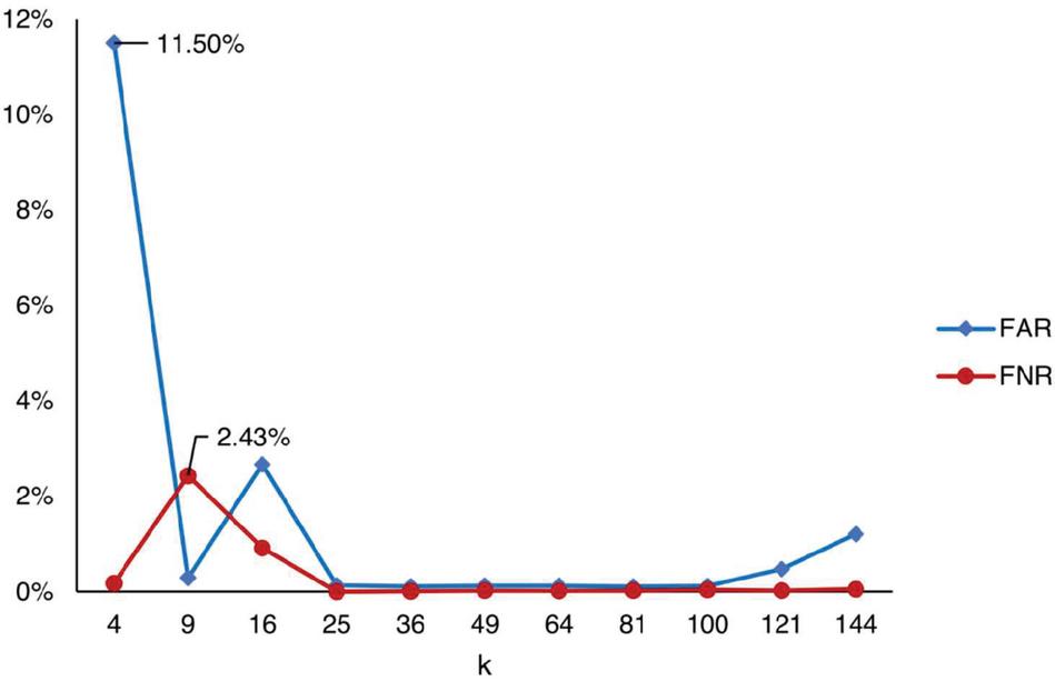
Figure 10 FAR and FNR.
4.6 Effects of Feature Importance and Writing Deformation
The nature of our method requires the selection of some features that are not very important. We therefore delve deeper into the effect of feature importance and writing deformation on our method. We used average F1 score from balanced and imbalanced dataset, cumulative features importance score, and pixels per grid, see Figure 11. The F1 score shows a high value and starts to stabilize when the cumulative feature importance score is 0.89 or at k 25. We argue that this is the threshold value of k needed in our method to get the best performance.
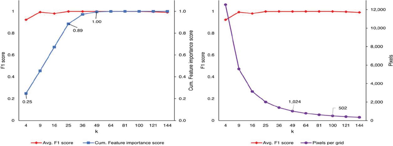
Figure 11 F1 score vs cumulative feature importance score (left) and F1 score vs pixels per grid (right).
Furthermore, we note that at k 9, the performance is already the best when cumulative feature importance score is only at 0.45. We assume that this may be an anomaly, where the features selected are enough to provide sufficient information. Whoever after we analyzed FAR and FNR at k 9, we found that the false negative rate for k 9 is relatively high while the false alarm rate is low. This indicate that at k 9, our trained models have poor performance despite their high F1 score.
We also noticed that at k 121, the performance slowly deteriorated. We argue that this might be because the additional features we add have a noise effect that affects performance, causing overfit. In addition, we believe that this is also due to the effect of the writing deformation on the image projection. Reducing pixels per grid, as can be seen in Figure 9, makes the text on the image unreadable.
We previously mentioned that writing begins to be unreadable by humans at k 49, this does not seem to apply to the model we were trained. The model starts struggling to classify at k 121. We conclude that when we add more features at this point, it creates its own noise by deforming the writing instead of enriching the information. Furthermore, we argue that k 100 is an upper limit in adding features. The suggested method uses the convolutional neural network (CNN) approach to learn the deep frequency features by using a plain rectangular filter with a modified pooling strategy that have more discriminative power for the SER. The proposed CNN model was trained on the extracted frequency features from the speech data and was then tested to predict the emotions.
5 Comparison with State-Of-The-Art Methods
We compared our method with several statistical models that we trained on tabular data. We used the exact same train set and test set (balanced and unbalanced). We trained Random Forest, SVM (RBF kernel), and XGBoost 3 times with the same k values as our CNN model. Random Forest was chosen because we used it as our feature ranking algorithm. Meanwhile, SVM and XGBoost were selected to provide a better understanding of the performance of our CNN model. The results can be seen in Table 3, we highlighted the best k values and the best model that has the best performance.
Table 3 Comparison with statistical models
| Random Forest | SVM (RBF) | XGB | CNN | |||||
| Rank | F1 score | Accuracy | F1 score | Accuracy | F1 score | Accuracy | F1 score | Accuracy |
| 4 | 92.78% | 91.25% | 70.45% | 63.52% | 92.78% | 91.24% | 92.27% | 90.62% |
| 9 | 99.49% | 99.50% | 71.19% | 64.40% | 99.45% | 99.45% | 99.29% | 99.30% |
| 16 | 99.68% | 99.68% | 85.02% | 81.35% | 99.64% | 99.64% | 97.97% | 97.66% |
| 25 | 99.93% | 99.93% | 85.73% | 81.92% | 99.92% | 99.92% | 99.89% | 99.89% |
| 36 | 99.95% | 99.95% | 96.59% | 96.31% | 99.94% | 99.94% | 99.91% | 99.91% |
| 49 | 99.95% | 99.95% | 96.88% | 96.65% | 99.95% | 99.95% | 99.89% | 99.89% |
| 64 | 99.95% | 99.95% | 97.19% | 97.00% | 99.95% | 99.95% | 99.89% | 99.89% |
| 81 | 99.95% | 99.95% | 96.60% | 96.35% | 99.95% | 99.95% | 99.91% | 99.91% |
| 100 | 99.94% | 99.94% | 95.77% | 95.37% | 99.95% | 99.95% | 99.90% | 99.90% |
| 121 | 99.94% | 99.94% | 95.72% | 95.31% | 99.95% | 99.95% | 99.61% | 99.61% |
| 144 | 99.95% | 99.95% | 95.70% | 95.28% | 99.95% | 99.95% | 99.02% | 99.00% |
The combination with the best performance is XGBoost at k values 81,100, 121, and 144. Whoever Random Forest has the best performance on the most k values (4, 9, 16, 25, 36, and 49). If we take the average of F1 score and accuracy across k, the rankings are (1) Random Forest, (2) XGBoost, (3) our CNN model, and (4) SVM. The performance difference between our model with Random Forest and XGBoost is very small, between 0.35% and 0.40%. From these results alone, we argue that our model is comparable to the statistical model.
However, there is a large gap in the time required to train between our CNN model and statistical model. The time required to train the statistical model was less than 10 minutes, while the time required to train our CNN model was approximately an hour. Despite its success in classifying tabular data sets using image projection, implementing CNN has a major drawback in the time it takes to train the model.
| Problem | SPH | B&B | TS | |||||||||
| No. | ||||||||||||
| 1 | 117 | 117 | 16.7 | 0 | 121 | 121 | 25.7 | 0 | 117 | 119.446 | 4920 | 0.00162 |
| 2 | 143.17 | 143.17 | 15.3 | 0 | 143.17 | 143.17 | 25.9 | 0 | 143.17 | 145.12 | 11,100 | 0.0002 |
| 3 | 121.58 | 121.58 | 13.9 | 0 | 121.58 | 121.58 | 23.9 | 0 | 122.57 | 124.093 | 13,847 | 0.00016 |
| 4 | 103.28 | 103.28 | 15.5 | 0 | 103.28 | 103.28 | 26.1 | 0 | 103.28 | 106.583 | 23,350 | 0.00184 |
| 5 | 92.95 | 92.95 | 15.2 | 0 | 105.9 | 105.9 | 23.9 | 0 | 92.95 | 101.29 | 37,544 | 0.00738 |
| 6 | 94.13 | 94.13 | 15.5 | 0 | 94.13 | 94.13 | 34.2 | 0 | 94.13 | 99.97 | 38,026 | 0.00847 |
| 7 | 92.95 | 92.95 | 15.3 | 0 | 92.95 | 92.95 | 60.9 | 0 | 92.95 | 101.77 | 39,962 | 0.01106 |
| 8 | 94.96 | 94.96 | 15.4 | 0 | 94.96 | 94.96 | 99.7 | 0 | 94.96 | 103.48 | 41,119 | 0.00962 |
| 9 | 84.25 | 84.5 | 31.4 | 0 | 84.25 | 84.5 | 153.5 | 0 | 84.79 | 104.26 | 44,592 | 0.01629 |
6 Conclusion
This study proposed a novel projection method of tabular data into image-based data that can be fed to convolutional neural networks classifiers. We built the IDS module leveraging the EfficienNet to reduce the computation load to suit IoT networks. We project the tabular data of wireless attacks into images by exploiting the zigzag sequences of attributes placed in a matrix. Each attribute value represents the matrix values in the dataset. Using the essential attributes using Feature Ranking and EfficientNet classifier, we achieved the best performance with 99.91% of F1 score. We also successfully maintain the false positive rate of about 0.11%. We also compared the proposed model with other machine learning models, and it is shown that our proposed model achieved comparable results with the other three models. We believe the spatial information must be considered by projecting the tabular data into grid-like data.
In the future, the methods to put the attribute sequence in the grid might be affected the image data for classification. In addition, a more lightweight model should be considered when implementing IDS for IoT networks.
Acknowledgment
This research was conducted under a contract of 2021 International Publication Assistance Q1 of Universitas Indonesia.
Funding Statement
This research was conducted under a contract of 2021 International Publication Assistance Q1 of Universitas Indonesia.
Conflicts of Interest
The Authors declare that they have no conflicts of interest to report regarding the present study.
References
[1] B. Tushir, Y. Dalal, B. Dezfouli and Y. Liu, “A quantitative study of ddos and e-ddos attacks on wifi smart home devices,” IEEE Internet of Things Journal, vol. 8, no. 8, pp. 6282–6292, 2021.
[2] T. Alam, “Cloud-Based IoT Applications and Their Roles in Smart Cities,” Smart Cities, vol. 4, no. 3, pp. 1196–1219. 2021.
[3] S. Brotsis, K. Limniotis, G. Bendiab, N. Kolokotronis and S. Shiaeles, “On the suitability of blockchain platforms for IoT applications: Architectures, security, privacy, and performance,” Computer Networks, vol. 191, pp. 108005, 2021.
[4] A. Jalal, M. A. Quaid and M. A Sidduqi, “A Triaxial acceleration-based human motion detection for ambient smart home system,” in 2019 16th International Bhurban Conference on Applied Sciences and Technology (IBCAST), Islamabad, Pakistan, pp. 353–358, 2019.
[5] M. Asaad, F. Ahmad, M. S. Alam and M. Sarfraz, “Smart grid and Indian experience: A review,” Resources Policy, vol. 74, pp. 101499, 2021.
[6] R. Guo, “Survey on wifi infrastructure attacks,” International Journal of Wireless and Mobile Computing, vol. 16, no. 2, pp. 97–101, 2019.
[7] S. J. Lee, D. Y. Paul, A. T. Asyhari, Y. Jhi, L. Chermak et al., “IMPACT: Impersonation attack detection via edge computing using deep autoencoder and feature abstraction,” IEEE Access, vol. 8, pp. 65520–65529, 2020.
[8] L. Qian, Z. Zhu, J. Hu and S. Liu, “Research of SQL injection attack and prevention technology,” in 2015 International Conference on Estimation, Detection and Information Fusion (ICEDIF), Harbin, China, pp. 303–306, 2015.
[9] E. Fazeldehkordi, I. S. Amiri and O. A. Akanbi, A Study of Black Hole Attack Solutions: On AODV Routing Protocol in MANET, 1st ed., Waltham, MA, USA: Syngress, 2016.
[10] P. Ioulianou, V. Vasilakis, I. Moscholios and M. Logothetis, “A signature-based intrusion detection system for the Internet of Things,” in Information and Communication Technology Form (ICTF), Graz, Austria, 2018.
[11] V. V. R. P. V. Jyothsna, R. Prasad and K. M. Prasad, “A Review of Anomaly Based Intrusion Detection Systems,” International Journal of Computer Applications, vol. 28, no. 7, pp. 26–35, 2011.
[12] A. A. Hady, A. Ghubaish, T. Salman, D. Unal and R. Jain, “Intrusion detection system for healthcare systems using medical and network data: A comparison study,” IEEE Access, vol. 8, pp. 106576–106584, 2020.
[13] M. Tan and Q. V. Le, “EfficientNet: rethinking Model Scaling for Convolutional Neural Networks,” in Proceedings of the 36th International Conference on Machine Learning, Long Beach, California, USA, pp. 6105–6114, 2019.
[14] S. Smys, A. Basar and H. Wang, “Hybrid intrusion detection system for internet of Things (IoT),” Journal of ISMAC, vol. 2, no. 04, pp. 190–199, 2020.
[15] M. A. Khan and J. Kim, “Toward developing efficient Conv-AE-based intrusion detection system using heterogeneous dataset,” Electronics, vol. 9, no. 11, pp. 1771, 2020.
[16] X. Li, W. Chen, Q. Zhang and L Wu, “Building auto-encoder intrusion detection system based on random forest feature selection.,” Computers & Security, vol. 95, pp. 101851, 2020.
[17] D. Jin, Y. Lu, J. Qin, Z. Cheng and Z. Mao, “SwiftIDS: Real-time intrusion detection system based on LightGBM and parallel intrusion detection mechanism,” Computers & Security, vol. 97, pp. 101984, 2020.
[18] M. A. Rahman, A. T. Asyhari, L. S. Leong, G. B. Satrya, M. H. Tao et al., “Scalable machine learning-based intrusion detection system for IoT-enabled smart cities,” Sustainable Cities and Society, vol. 61, pp. 102324, 2020.
[19] S. N. Mighan and M. Kahani, “A novel scalable intrusion detection system based on deep learning,” International Journal of Information Security, vol. 20, no. 3, pp. 387–403, 2021.
[20] I. Al-Turaiki and N. Altwaijry, “A convolutional neural network forimproved anomaly-based network intrusion detection,” Big Data, vol. 9, no. 3, pp. 233–252, 2021.
[21] M. Popescu and A. Naaji, “Chapter 3 – detection of small tumors of thebrain using medical imaging,” in Handbook of Decision Support Systems for Neurological Disorders. Cambridge, MA, USA: Academic Press, pp. 33–53, 2021. [Online]. Available: https://www.sciencedirect.com/science/article/pii/B978012822271300013X
[22] G. K. Wallace, “The JPEG still picture compression standard,” IEEE Transactions on Consumer Electronics, vol. 38, no. 1, pp. xviii–xxxiv, 1992.
Biography

Hailyie Tekleselassie W/michael holds a BSc degree in Information Systems from University of Gondar, and MSc degree in Information Systems from Addis Ababa University. His current research interests are: Cyber Security, Big Data, AI, ICT and Mobile Computing. He currently Lecturer at Wolaita Sodo University, He is a member of the Ethiopian Space Science Society (ESSS) and the Institution of Electrical and Electronics Engineers (IEEE).
Journal of Cyber Security and Mobility, Vol. 11_4, 601–620.
doi: 10.13052/jcsm2245-1439.1145
© 2022 River Publishers