On the Use of the Kolmogorov–Wiener Filter for Heavy-tail Process Prediction

Vyacheslav Gorev^*, Alexander Gusev, Valerii Korniienko and Yana Shedlovska

Dnipro University of Technology, Dnipro, Ukraine
E-mail: lordjainor@gmail.com
*Corresponding Author

Received 28 October 2022; Accepted 18 January 2023; Publication 16 May 2023

Abstract

This paper is devoted to the investigation of the applicability of the Kolmogorov–Wiener filter to the prediction of heavy-tail processes. As is known, telecommunication traffic in systems with data packet transfer is considered to be a heavy-tail process. There are a lot of rather sophisticated approaches to traffic prediction; however, in the rather simple case of stationary traffic sophisticated approaches may not be needed, and a simple approach, such as the Kolmogorov–Wiener filter, may be applied. However, as far as we know, this approach has not been considered in recent papers. In our previous papers, we theoretically developed a method for obtaining the filter weight function in the continuous case. The Kolmogorov–Wiener filter may be applied only to stationary processes, but in some models telecommunication traffic is treated as a stationary process, and thus the use of the Kolmogorov–Wiener filter may be of practical interest. In this paper, we generate stationary heavy-tail modeled data similar to fractional Gaussian noise and investigate the applicability of the Kolmogorov–Wiener filter to data prediction. Both non-smoothed and smoothed processes are investigated. It is shown that both the discrete and the continuous Kolmogorov–Wiener filter may be used in a rather accurate short-term prediction of a heavy-tail smoothed stationary random process. The paper results may be used for stationary telecommunication traffic prediction in systems with packet data transfer.

Keywords: Discrete Kolmogorov–Wiener filter, continuous Kolmogorov–Wiener filter, heavy-tail process, telecommunication traffic prediction.

1 Introduction

Telecommunication traffic prediction is an important problem. For example, it is important for the effective use of resource management, for network planning, for cyber security (suspicious traffic identification), etc. [1, 2].

There are a variety of different approaches to traffic prediction reported in the recent literature. For example, the following approaches are presented in recent papers: the ARMA and the ARIMA approaches and their modifications [3, 4], the GARCH model and its improvements [5, 6], neural networks, artificial intelligence and deep learning [7–10], hybrid methods [11–13], the Holt-Winters approach [14], the gray Markov Verhulst model [15], the wavelet transform [16], the Prophet approach [17], etc.

There are many different telecommunication traffic models, including stationary ones, for example, such as the fractional Gaussian noise model, the generalized fractional Gaussian noise model [18], the Gaussian fractional sum-difference model (see [19] and references in [19]), the power-law structure function model [20], etc. Nowadays telecommunication traffic in systems with data packet transfer is treated as a heavy-tail random process; in other words, the traffic correlation function is considered to have asymptotic power-law decay, see, for example, [21].

Such a simple prediction algorithm as the Kolmogorov–Wiener filter may be applied to the prediction of and noise cancellation in stationary processes [22]. This filter is rather widely used in different fields of knowledge, for example, in signal treatment [23], in econometrics [24], in image treatment [25], in atmosphere investigation [26], in the investigation of biological cellular sensing systems [27], etc. However, as far as we know, this filter is not considered in recent papers devoted to telecommunication traffic. In our opinion, the use of such a filter for traffic prediction in simple stationary cases may be of interest because of its simplicity, especially in the discrete case. We know only few papers where this filter is applied to telecommunication traffic treatment, and they are not recent ones. In paper [28], it is used for traffic noise cancellation. In paper [29], the one-point-forward Kolmogorov–Wiener prediction of a noisy traffic is investigated; in paper [30], the one-point forward and five-point-forward Kolmogorov–Wiener prediction of a non-smoothed fractional Gaussian noise traffic is investigated. In paper [30], it is indicated that the predicted signal follows the original one, but with a smaller amplitude. In [30] only the discrete Kolmogorov–Wiener filter was used, and non-smoothed processes were considered. Papers [28–30] are devoted to a prediction on the basis of a discrete filter.

In this paper. we deal with the prediction of a non-noisy heavy-tail process. Our preliminary results are published in [31] where we used the symmetric moving average approach in order to generate modeled data of a heavy-tail fractional Gaussian noise process. In [31] we investigated the discrete Kolmogorov–Wiener prediction for the corresponding non-smoothed process and smoothed process obtained by a simple linear smoothing method. In our papers [20, 32–34] it is shown that in the continuous case the Galerkin method may be applied to finding the Kolmogorov–Wiener filter weight function for the prediction of heavy-tail processes in different models. In [20, 32–34] we restricted ourselves only to the investigation of the weight function rather than the prediction itself, so the investigation of the corresponding prediction is one of the aims of the paper.

The aim of this paper is to investigate the Kolmogorov–Wiener prediction for modeled heavy-tail data for different smoothing algorithms and to investigate both discrete and continuous approaches to the Kolmogorov–Wiener prediction of a heavy-tail process.

The scientific novelty of the paper is as follows.

1. It is shown that the Kolmogorov–Wiener filter (both discrete and continuous) may be used in a rather accurate short-term prediction of a heavy-tail smoothed stationary random process, which may be useful for traffic prediction in stable stationary systems and for the prediction of noisy processes after the truncation of the random component.

2. The modeled data for two heavy-tail processes (with Hurst exponents H $=$ 0.8 and H $=$ 0.6) are investigated. It is shown that the Kolmogorov–Wiener filter prediction gives better results for the smoothed process with the higher Hurst exponent.

It should be stressed that the aim of the paper is to illustrate the fact that the Kolmogorov–Wiener filter may be used in the prediction of stationary smoothed heavy-tail processes rather than to compare the Kolmogorov–Wiener prediction with other prediction techniques reported in the literature. The simplicity of the Kolmogorov–Wiener filter in comparison, for example, with neural networks may be its advantage, and a detailed comparison may be the subject of another paper.

The paper is organized as follows. In Section 1, the introduction is given; in Section 2, a description of the Kolmogorov–Wiener filter in the discrete and the continuous case is made and the heavy-tail data generated in [31] are described. In Sections 3 and 4, the prediction is investigated in the discrete and the continuous case, respectively. In Section 5, a discussion is given, and in Section 6, conclusions are made.

2 Kolmogorov–Wiener Filter and Generation of Modeled Heavy-tail Data

In this paper, we investigate only the prediction (without noise cancellation) based on the Kolmogorov–Wiener filter; the process is considered to be non-noisy. Let us first consider the discrete case. Let us have a stationary process $x_t$ to be predicted. Let us make a $z$-point-forward prediction on the basis of $T+1$ previous points. The Kolmogorov–Wiener filter output $y_t$ is as follows [22]:

$$y_t=\sum _{i=0}^T{h}_i{x}_{t-i}$$

(1)

where the weight coefficients $h_i,i=\overline{0,T}$ may be obtained in matrix form:

$\left(\begin{array}{c}\hfill h_0\hfill \\ \hfill h_1\hfill \\ \hfill h_2\hfill \\ \hfill \mathrm{⋮}\hfill \\ \hfill h_T\hfill \end{array}\right)$	$={\left(\begin{array}{ccccc}\hfill R_x(0)\hfill & \hfill R_x(1)\hfill & \hfill R_x(2)\hfill & \hfill \mathrm{\cdots }\hfill & \hfill R_x(T)\hfill \\ \hfill R_x(1)\hfill & \hfill R_x(0)\hfill & \hfill R_x(1)\hfill & \hfill \mathrm{\cdots }\hfill & \hfill R_x(T-1)\hfill \\ \hfill R_x(2)\hfill & \hfill R_x(1)\hfill & \hfill R_x(0)\hfill & \hfill \mathrm{\cdots }\hfill & \hfill R_x(T-2)\hfill \\ \hfill \mathrm{⋮}\hfill & \hfill \mathrm{⋮}\hfill & \hfill \mathrm{⋮}\hfill & \hfill \mathrm{\ddots }\hfill & \hfill \mathrm{⋮}\hfill \\ \hfill R_x(T)\hfill & \hfill R_x(T-1)\hfill & \hfill R_x(T-2)\hfill & \hfill \mathrm{\cdots }\hfill & \hfill R_x(0)\hfill \end{array}\right)}^{-1}$
	$\mathrm{\hspace{1em}}\cdot \left(\begin{array}{c}\hfill R_x(z)\hfill \\ \hfill R_x(z+1)\hfill \\ \hfill R_x(z+2)\hfill \\ \hfill \mathrm{⋮}\hfill \\ \hfill R_x(z+T)\hfill \end{array}\right),$	(2)

$R_x(t)$ is the correlation function of the process $x_t$. The value $y_t$ is the predicted value of $x_{t+z}$.

In the continuous case, let us have a stationary process $x(t)$. The prediction for $x(t+z)$ is made on the basis of the values $x(t),t\in [0,T]$. Then the filter output $y(t)$, which is the prediction for $x(t+z)$, may be calculated as follows:

$$y(t)={\int }_0^{T}h(\tau )x(t-\tau )\mathit{d}\tau$$

(3)

where the filter weight function $h(t)$ is the solution of the Wiener–Hopf integral equation [22]

$${\int }_0^{T}h(\tau )R_x(t-\tau )\mathit{d}\tau =R_x(t+z).$$

(4)

In [20, 32–34], we showed that the Galerkin method may be used in order to obtain an approximate solution for $h(\tau )$. The idea of the method is as follows. The approximate solution in the approximation of $n$ functions is sought in the form

$$h(\tau )=\sum _{s=0}^{n-1}{g}_s{S}_s(\tau )$$

(5)

where $S_0(\tau ),S_1(\tau ),\mathrm{\dots }$ is a complete orthogonal function system. The coefficients $g_s$ may be expressed in matrix form

$$\left(\begin{array}{c}\hfill g_0\hfill \\ \hfill g_1\hfill \\ \hfill \mathrm{⋮}\hfill \\ \hfill g_{n-1}\hfill \end{array}\right)={\left(\begin{array}{cccc}\hfill G_{00}\hfill & \hfill G_{01}\hfill & \hfill \mathrm{\cdots }\hfill & \hfill G_{0,n-1}\hfill \\ \hfill G_{10}\hfill & \hfill G_{11}\hfill & \hfill \mathrm{\cdots }\hfill & \hfill G_{1,n-1}\hfill \\ \hfill \mathrm{⋮}\hfill & \hfill \mathrm{⋮}\hfill & \hfill \mathrm{\ddots }\hfill & \hfill \mathrm{⋮}\hfill \\ \hfill G_{n-1,0}\hfill & \hfill G_{n-1,1}\hfill & \hfill \mathrm{\cdots }\hfill & \hfill G_{n-1,n-1}\hfill \end{array}\right)}^{-1}\cdot \left(\begin{array}{c}\hfill B_0\hfill \\ \hfill B_1\hfill \\ \hfill \mathrm{⋮}\hfill \\ \hfill B_{n-1}\hfill \end{array}\right)$$

(6)

where

$G_{ij}={\displaystyle {\int }_0^T}{\displaystyle {\int }_0^T}{S}_i(\tau )S_j(t)R_x(t-\tau )\mathit{d}t\mathit{d}\tau ,B_i={\displaystyle {\int }_0^T}{S}_i(t)R_x(t+z)\mathit{d}t.$

For example, the following systems of functions $S_s(\tau )$ may be chosen: orthogonal polynomial systems (the Chebyshev polynomials of the first and of the second kind), trigonometric functions, which form a trigonometric Fourier series, and the Walsh functions.

In this paper, we deal with the modeled heavy-tail fractional Gaussian noise data $X_i$ generated in [31] on the basis of the symmetric moving average approach using the following formulas:

$$X_i=\sum _{j=-q}^q{a}_{|j|}{V}_{i+j+q},a_0=\frac{\sqrt{2-2H}}{1.5-H}{\gamma }_0,$$
$$a_j=\frac{a_0}{2}({(j+1)}^{H+0.5}+{(j-1)}^{H+0.5}-2j^{H+0.5})$$	(8)

where $H$ is the Hurst parameter and ${\gamma }_0$ is the variance of the process $X_i$; $V_i$ is a stationary white noise with a variance equal to 1 and an average value equal to 0. The following parameters are used [31]: $q=3\cdot {10}^5$, ${\gamma }_0=1\cdot {10}^5$ points of the process $X_i$ are generated. The average value of the process $X_i$ is close to zero, and, obviously, the traffic should be a non-negative process, so the modeled traffic data are as follows:

$$x_i=X_i+\min (X)+{10}^{-3},$$

(9)

a small value 10${}^{-3}$ is added in order to avoid an infinite mean absolute percentage error. In this paper, we generate data for a process with Hurst exponent $H=0.8$ and for a process with Hurst exponent $H=0.6$.

3 Investigation of the Prediction in the Discrete Case

3.1 Investigation of the Case of a Non-smoothed Process

A centralized process should be constructed first:

$$x{c}_i=x_i-⟨x⟩$$

(10)

where $⟨x⟩$ is the average value of the process $x_i$. The corresponding correlation function is calculated as

$$R_x(t)=\frac{1}{{10}^5-\tau }\sum _{i=1}^{{10}^5-\tau }x{c}_{i}x{c}_{i+\tau }.$$

(11)

Let us investigate the prediction of a non-smoothed process. Let us make a $z$-point-forward prediction on the basis of $T+1$ previous points. The filter weight coefficients $h_i,i=\overline{0,T}$ are calculated on the basis of (2) and (11). At the first iteration, we take the first $T+1$ points (points with numbers from 1 to $T+1$) and on their basis we calculate the prediction for $x{c}_{T+2},x{c}_{T+3},\mathrm{\dots },x{c}_{T+z+1}$. At the second iteration, we take the points with numbers from 2 to $T+2$ and on their basis we calculate the prediction for $x{c}_j,j=\overline{T+3,T+z+2}$. And so on throughout the whole array. At iteration number $i$, we calculate the predicted values according to (1) as follows:

$x{c}_k^{\prime }=x{c}_{k+i},k=\overline{0,T};\widehat{x{c}_{j+z}}={\displaystyle \sum _{k=0}^j}{h}_{k}x{c}_{j-k}^{\prime },j=\overline{T-z+1,T}.$

Here the upper bound of summation in (3.1) is changed in comparison with expression (1) in order to avoid dealing with indices beyond the filter input data. Such a change does not have any significant effect on the result because only the cases $T\gg z$ are investigated. In what follows, a similar change is made. In (3.1) and in what follows, the designation $\widehat{a}$ means the predicted value of $a$. Thus, the predicted modeled traffic values are

$$\widehat{x_j}=\widehat{x{c}_j}+⟨x⟩$$

(13)

and the corresponding mean absolute percentage error (MAPE) and mean average error (MAE) at the $i$th iteration are as follows:

${\mathrm{MAPE}}_i$	$={\displaystyle \frac{1}{z}}{\displaystyle \sum _{j=T+1+i}^{T+z+i}}\left|{\displaystyle \frac{x_j-\widehat{x_j}}{x_j}}\right|\cdot 100\%,$
${\mathrm{MAE}}_i$	$={\displaystyle \frac{1}{z}}{\displaystyle \sum _{j=T+1+i}^{T+z+i}}|x_j-\widehat{x_j}|.$	(14)

The number of iterations is equal to ${10}^5-T-z$; the average prediction errors over the whole array are calculated:

$\mathrm{MAPE}$	$={\displaystyle \frac{1}{{10}^5-T-z}}{\displaystyle \sum _{i=1}^{{10}^5-T-z}}{\mathrm{MAPE}}_i,$
$\mathrm{MAE}$	$={\displaystyle \frac{1}{{10}^5-T-z}}{\displaystyle \sum _{i=1}^{{10}^5-T-z}}{\mathrm{MAE}}_i.$	(15)

The results for the non-smoothed process are given in Tables 1 and 2.

Table 1 Non-smoothed process MAPE (%)

	$H=0.8$					$H=0.6$
	$z=1$	$z=2$	$z=3$	$z=4$	$z=5$	$z=1$	$z=2$	$z=3$	$z=4$	$z=5$
$T=100$	24.7	25.3	25.4	25.7	25.9	25.5	25.6	25.6	25.6	25.6
$T=1000$	24.5	25.0	25.1	25.3	25.6	25.3	25.4	25.4	25.5	25.5

Table 2 Non-smoothed process MAE

	$H=0.8$					$H=0.6$
	$z=1$	$z=2$	$z=3$	$z=4$	$z=5$	$z=1$	$z=2$	$z=3$	$z=4$	$z=5$
$T=100$	0.697	0.710	0.717	0.723	0.727	0.792	0.793	0.794	0.794	0.794
$T=1000$	0.694	0.707	0.714	0.719	0.723	0.788	0.789	0.790	0.790	0.790

The results in Tables 1 and 2 are rounded off to 3 significant digits. The average value is $⟨x⟩=3.88$ for $H=0.8$ and $⟨x⟩=4.25$ for $H=0.6$. In the case $T=100$, $z=1$, $H=0.8$ a graphical comparison of the actual and the predicted modeled traffic values is given in Figure 1 (the solid line is the actual process, and the dotted line is the predicted one). In fact, a picture similar to the results of paper [30] is obtained: the predicted signal is in some sense similar to the original one, but with a smaller amplitude. Thus, the prediction illustrates the process tendency, but particular values may not be in good agreement.

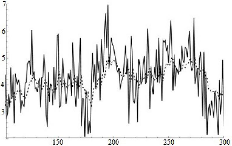
Figure 1 Comparison of the actual and the predicted values of the non-smoothed process for $T=100$ and $z=1$; $H=0.8$.

3.2 Investigation of the Case of a Smoothed Process

Let us investigate the case of a heavy-tail process smoothed by the simple linear smoothing algorithm:

$${\tilde{X}}_i=\frac{1}{2l+1}\sum _{j=-l}^l{X}_{i+j}.$$

(16)

Table 3 MAPE (%) for a process smoothed on the basis of (16), $T=100$

	$H=0.8$					$H=0.6$
	$z=1$	$z=2$	$z=3$	$z=4$	$z=5$	$z=1$	$z=2$	$z=3$	$z=4$	$z=5$
$l=1$	9.11	15.1	20.3	20.9	21.4	13.3	20.1	25.6	25.7	25.7
$l=2$	6.26	10.2	13.8	17.2	21.2	8.86	13.3	16.9	20.1	23.5
$l=3$	4.85	7.86	10.4	13.2	15.9	7.55	11.3	13.9	16.4	18.8
$l=4$	3.92	6.13	8.07	10.0	12.0	6.49	9.66	11.9	14.1	16.1
$l=5$	3.37	5.30	6.97	8.64	10.3	5.71	8.25	10.4	12.3	14.1

Table 4 MAE for a process smoothed on the basis of (16) , $T=100$

	$H=0.8$					$H=0.6$
	$z=1$	$z=2$	$z=3$	$z=4$	$z=5$	$z=1$	$z=2$	$z=3$	$z=4$	$z=5$
$l=1$	0.234	0.365	0.480	0.493	0.501	0.267	0.387	0.481	0.482	0.482
$l=2$	0.142	0.221	0.291	0.356	0.418	0.162	0.235	0.292	0.341	0.384
$l=3$	0.103	0.160	0.210	0.257	0.302	0.116	0.170	0.210	0.246	0.277
$l=4$	0.0810	0.125	0.165	0.202	0.238	0.0916	0.133	0.165	0.193	0.218
$l=5$	0.0665	0.103	0.137	0.168	0.197	0.0759	0.110	0.136	0.160	0.180

In [31], it is shown that the process ${\tilde{X}}_i$ is also a heavy-tail one. Then the modeled traffic data $x_i$ are as follows:

$$x_i={\tilde{X}}_i+\min (\tilde{X})+{10}^{-3},$$

(17)

and the prediction algorithm based on formulas (10)–(3.1) is the same. The results for the smoothed process at different values of $l$ are given in Tables 3–6. Its average values are given in Table 7. As can be seen, the prediction results are much better in the case of a smoothed process. It can also be seen that the prediction error increases with increasing $z$ and such an increase may be significant, especially for $l=1$. Therefore, one can conclude that the Kolmogorov–Wiener filter may be applied only to a short-term prediction of a heavy-tail process. As can be seen, the results for $T=1000$ are slightly better than for $T=100$, but the difference is not significant. It should also be stressed that the prediction results for the case where $H=0.8$ are better than those for the case where $H=0.6$.

Table 5 MAPE (%) for a process smoothed on the basis of (16), $T=1000$

	$H=0.8$					$H=0.6$
	$z=1$	$z=2$	$z=3$	$z=4$	$z=5$	$z=1$	$z=2$	$z=3$	$z=4$	$z=5$
$l=1$	9.00	14.9	20.2	20.9	21.3	13.1	19.9	25.4	25.5	25.5
$l=2$	6.14	9.96	13.6	16.9	21.0	8.74	13.1	16.7	19.9	23.4
$l=3$	4.78	7.72	10.2	13.0	15.7	7.41	11.1	13.7	16.2	18.6
$l=4$	3.84	5.95	7.80	9.69	11.7	6.38	9.48	11.7	13.8	15.8
$l=5$	3.28	5.11	6.64	8.25	9.92	5.59	8.03	10.1	12.0	13.7

Table 6 MAE for a process smoothed on the basis of (16), $T=1000$

	$H=0.8$					$H=0.6$
	$z=1$	$z=2$	$z=3$	$z=4$	$z=5$	$z=1$	$z=2$	$z=3$	$z=4$	$z=5$
$l=1$	0.232	0.362	0.477	0.490	0.498	0.264	0.384	0.478	0.479	0.480
$l=2$	0.140	0.218	0.287	0.353	0.416	0.160	0.231	0.289	0.338	0.382
$l=3$	0.101	0.156	0.206	0.253	0.298	0.114	0.166	0.206	0.242	0.274
$l=4$	0.0790	0.122	0.160	0.197	0.232	0.0900	0.130	0.161	0.189	0.214
$l=5$	0.0650	0.100	0.131	0.161	0.190	0.0742	0.107	0.132	0.155	0.175

Table 7 Average values $⟨x⟩$ for the smoothed process (17)

$l$	$⟨x⟩$, $H=0.8$	$⟨x⟩$, $H=0.6$
1	2.98	2.45
2	2.52	2.06
3	2.34	1.77
4	2.31	1.61
5	2.22	1.48

The results in Tables 3–7 are rounded off to 3 significant digits. In the case $z=1$, $l=3$, $T=100$, $H=0.8$ a graphical comparison of the actual and the predicted modeled traffic values is given in Figure 2 (the solid line is the actual process, and the dotted line is the predicted one).

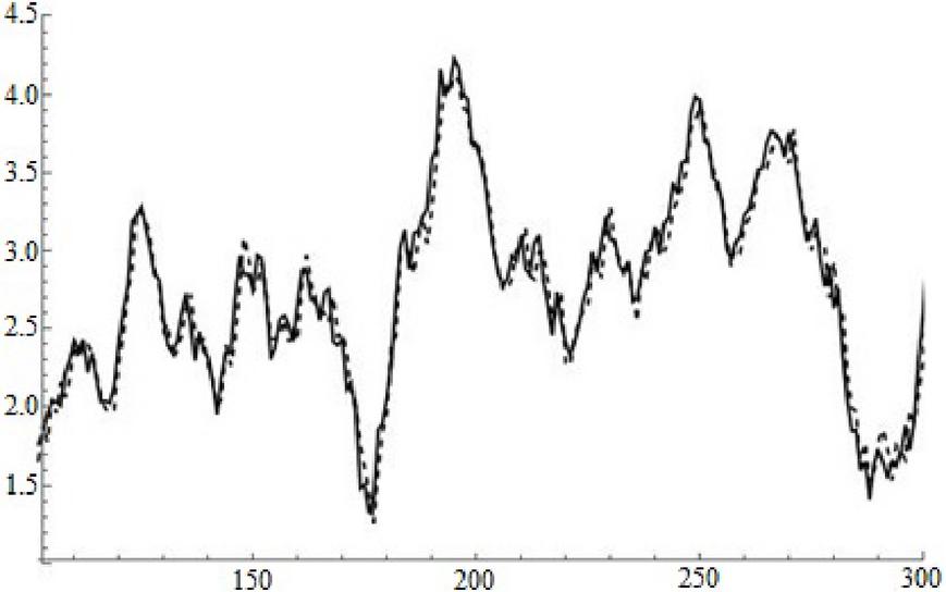
Figure 2 Comparison of the actual and the predicted values for a process smoothed on the basis of (16) for $T=100$, $z=1$, $l=3$; $H=0.8$.

As can be seen, the graphs in Figure 2 are indeed in good agreement.

Now let us consider a process smoothed in the basis of exponential average smoothing:

$$X_t^{\prime }=\frac{1-\lambda }{1-{\lambda }^t}\sum _{k=0}^{t-1}{\lambda }^k{X}_{t-k},\lambda =0.9.$$

(18)

Then the modeled traffic data $x_i$ are as follows:

$$x_i=X_i^{\prime }+\min (X^{\prime })+{10}^{-3},$$

(19)

and the prediction algorithm based on formulas (10)–(3.1) is the same. Let us show that the corresponding process is a heavy-tail one (its correlation function exhibits a power-law asymptotic decay). The correlation function of the corresponding centralized process with $H=0.8$ (the solid line) and its least-mean-squares estimate for the first 500 points (the dotted line) are given in Figure 3.

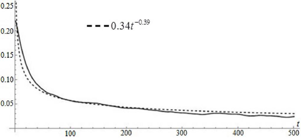
Figure 3 Correlation function of the centralized process obtained on the basis of (19) and its power-law least-squares fit; $H=0.8$.

As for the process with $H=0.6$, the corresponding proof is similar. As can be seen, the correlation function indeed exhibits a power-law asymptotic decay. The results for the MAPE and the MAE are shown in Tables 8 and 9.

Table 8 MAPE (%) for a process smoothed on the basis of (18)

	$H=0.8$					$H=0.6$
	$z=1$	$z=2$	$z=3$	$z=4$	$z=5$	$z=1$	$z=2$	$z=3$	$z=4$	$z=5$
$T=100$	4.03	6.09	7.84	9.20	10.4	8.21	11.7	13.9	15.7	17.2
$T=1000$	4.02	6.07	7.79	9.14	10.4	8.17	11.6	13.8	15.6	17.1

Table 9 MAE for a process smoothed on the basis of (18)

	$H=0.8$					$H=0.6$
	$z=1$	$z=2$	$z=3$	$z=4$	$z=5$	$z=1$	$z=2$	$z=3$	$z=4$	$z=5$
$T={10}^2$	0.0697	0.104	0.131	0.153	0.173	0.0792	0.110	0.131	0.147	0.159
$T={10}^3$	0.0694	0.103	0.130	0.153	0.172	0.0788	0.109	0.130	0.146	0.158

The results in Tables 8 and 9 are rounded off to 3 significant digits. The average value of the process is 1.91 for $H=0.8$ and 1.10 for $H=0.6$. As can be seen, a short-term Kolmogorov–Wiener prediction works well for the process under consideration, and the prediction in the case where $H=0.8$ is better than that for the case where $H=0.6$. The graphs for the actual and predicted values are given in Figure 4 for the process with $H=0.8$.

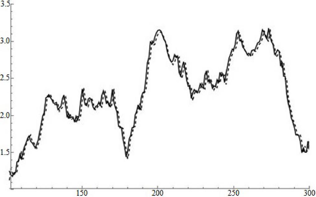
Figure 4 Comparison of the actual and the predicted values for a process smoothed on the basis of (18) for $T=100$, $z=1$; $H=0.8$.

In Figure 4, the solid line shows the actual values of the modeled traffic, and the dotted line shows the predicted values. It should also be stressed that for values of $\lambda$ smaller than that in (18) the corresponding prediction leads to higher errors.

4 Investigation of the Applicability of a Continuous Filter

This section is devoted to the investigation of the applicability of a continuous filter to traffic prediction. Of course, the actual traffic is discrete, and the use of a discrete filter is more exact, but the open question is to what extent the continuous Kolmogorov–Wiener filter is applicable to the corresponding prediction. In the continuous case, the filter weight function is the solution of the integral Equation (4), and thus a continuous process correlation function is needed. The least-squares estimate of the process correlation function may be used in this case.

First of all, let us consider the case where $H=0.8$. Let us suppose that a large amount of data is given during a rather short time interval, for example, 10${}^5$ data points are taken for a time period equal to 100 seconds, see Figure 5. In such a case, the process may be treated as continuous (however, of course, such a “continuousness” is rather artificial).

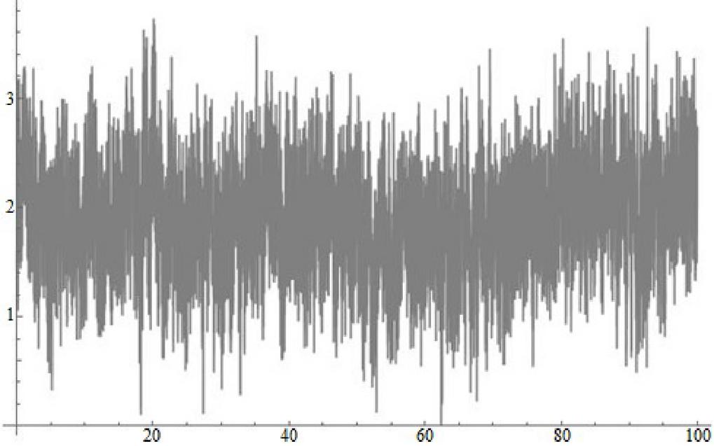
Figure 5 “Continuous” smoothed modeled traffic data obtained on the basis of exponential average smoothing; $H=0.8$.

Let us investigate the applicability of a continuous filter by the example of a process smoothed on the basis of (18). Let us consider the case where the filter input data are given for the previous $T=1$ second and the forecast for a future interval equal to $z={10}^{-3}$ seconds (analog of a discrete one-point-forward prediction on the basis of the previous 1001 points). First the corresponding centralized process $xc(t)$ is built, and the continuous correlation function of the process is taken as the least-squares estimate, see Figure 6 where the black line is the actual correlation function and the gray line is the least-squares estimate (20)

$$R_x(t)=a\cdot {(|t|+{10}^{-3})}^{-b},|t|\in [0,1],a=0.0206,b=0.415.$$

(20)

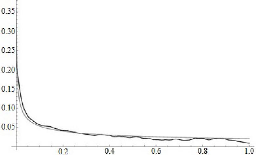
Figure 6 Comparison of the actual correlation function and its least squares (20); $H=0.8$.

The coefficients $a$ and $b$ appearing in (20) are rounded off to 3 significant digits; however, their exact values are used in the calculations. The term ${10}^{-3}$ is added to the denominator in (20) in order to take into account the fact that the process variance is finite. The evenness of the correlation function is also taken into account. The filter weight function $h(\tau )$ is calculated on the basis of (5)–(2) where the functions $S_s(\tau )$ are the Walsh functions in the Walsh numeration (see the description of these functions in [32]). At the first iteration, we take the time interval $t\in [0,T]$, and on its basis we calculate the prediction for $xc(T+z)$. At the second iteration, we take the time interval $t\in [z,T+z]$, and on its basis we calculate the prediction for $xc(T+2z)$. And so on throughout the whole array. At iteration number $i$, we calculate the predicted values according to (3) as follows, see (4).

$\widehat{xc}(T+iz)$	$={\displaystyle {\int }_0^T}h(\tau )xc(T+(i-1)\cdot z-\tau )\mathit{d}\tau$
	$\approx {\displaystyle \sum _{j=0,{10}^{-3},2\cdot {10}^{-3},\mathrm{\dots }}^{T-{10}^{-3}}}h(j)\cdot xc(T+(i-1)\cdot z-j)\cdot {10}^{-3},$

here, the integral is evaluated by the method of rectangles. Approximations of different numbers of Walsh functions are used. The results for the average values of the MAPE and the MAE are given in Table 10. In Table 10, $n$ is the number of Walsh functions in (5) and the results are rounded off to 3 significant digits. As can be seen, the more Walsh functions are taken, the more accurate the prediction is.

Table 10 MAPE (%) and MAE for the case under consideration in the continuous approximation for the correlation function (20); $H=0.8$

$n$	MAPE, %	MAE
32	15.4	0.243
64	13.6	0.213
128	9.71	0.155
256	7.94	0.126

This approach may be enhanced on the basis of the idea that the power-law behavior is an asymptotic behavior for long times, but for short times the function (20) does not describe the correlation function well. Thus, for short times another estimate may be made, for example, the polynomial one, and the improved least-squares fit may be as follows:

$$R_x(t)=\{\begin{array}{cc}{a}_1{|t|}^3+b_1{|t|}^2+c_1|t|+d_1,\hfill & |t|\in [0,0.1]\hfill \\ a\cdot {(|t|+{10}^{-3})}^{-b},\hfill & |t|\in (0.1,1]\hfill \end{array},$$
$$a_1=-369,b_1=79.0,c_1=-5.89,d_1=0.220.$$	(22)

The coefficients $a_1$, $b_1$, $c_1$, and $d_1$ appearing in (22) are rounded off to 3 significant digits; however, their exact values are used in the calculations. The coefficients $a$ and $b$ are taken from (20).

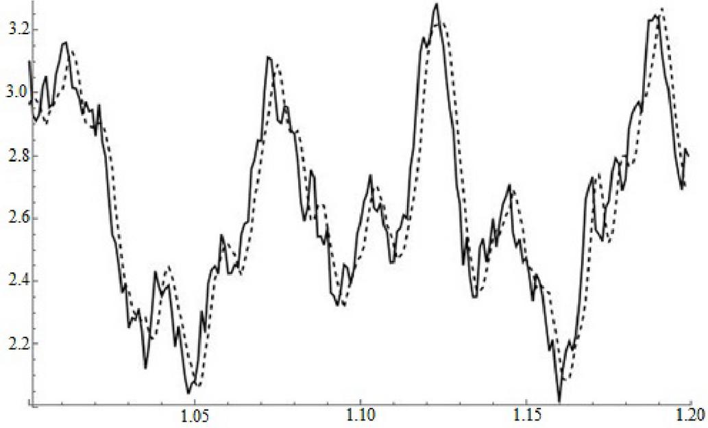
Figure 7 Comparison of the actual modeled traffic and the predicted one obtained on the basis of the continuous filter and the correlation function (22) in the approximation of 256 Walsh functions; $H=0.8$.

Of course, the function (22) has some drawbacks: it is not continuous at the points $|t|=0.1$ and its coefficients $a$ and $b$ may be refined on the basis of the idea that the corresponding least-squares fit can be made for $|t|\in (0.1,1]$, not for $|t|\in [0,1]$. However, as can be seen in what follows, the function (22) leads to reliable results, see Table 11. A graphical comparison is given in Figure 7.

In the case where $H=0.6$, a similar procedure may be realized, and the corresponding correlation function is as follows:

$$R_x(t)=\{\begin{array}{cc}{a}_1{|t|}^4+b_1{|t|}^3+c_1{|t|}^2+d_1|t|+e_1,\hfill & |t|\in [0,0.1]\hfill \\ a\cdot {(|t|+{10}^{-3})}^{-b},\hfill & |t|\in (0.1,1]\hfill \end{array},$$
$$a_1=6027,b_1=-1486,c_1=130.5,d_1=-4.923,e_1=0.07340,$$
$$a=8.089\cdot {10}^{-4},b=0.7130,$$	(23)

The coefficients in (23) are rounded off to 4 significant digits; however, their exact values are used in the calculations.

Table 11 MAPE (%) and MAE for the case under consideration in the continuous approximation for the correlation functions (22) and (23) for $H=0.8$ and $H=0.6$, respectively

	$H=0.8$		$H=0.6$
$n$	MAPE, %	MAE	MAPE, %	MAE
32	14.9	0.240	20.9	0.188
64	11.3	0.185	17.4	0.160
128	7.94	0.135	13.7	0.129
256	5.81	0.0986	10.8	0.104

The results in Table 11 are rounded off to 3 significant digits. As can be seen, the accuracy increases with the number of Walsh functions and the corresponding results are better than those indicated in Table 10. In Figure 7, the solid line is the actual modeled traffic and the dotted line is the predicted one. As can be seen, the prediction is rather accurate, and thus the continuous Kolmogorov–Wiener filter may be applied to the prediction of a heavy-tail process smoothed on the basis of (18). It should also be stressed that the corresponding prediction is better in the case where $H=0.8$ than in the case where $H=0.6$.

5 Discussion

This paper is an extension of the results presented at the IntelItSis 2022 Conference [31]. It is devoted to the investigation of the applicability of the Kolmogorov–Wiener filter to the prediction of a stationary heavy-tail random process similar to fractional Gaussian noise. The calculations presented in the paper were made on the basis of the Wolfram Mathematica package using a PC with processor Intel(R) Core(TM) i5-9400 CPU @ 2.90 GHz.

Modeled traffic data (10${}^5$ points) are generated on the basis of the symmetric moving average approach. The data are generated for two processes: for a process with Hurst exponent equal to 0.8 and for a process with Hurst exponent equal to 0.6. First the applicability of the Kolmogorov–Wiener filter to non-smoothed traffic is considered. The MAPE and MAE are rather high in this case, the predicted process behavior is rather similar to the actual one, but the amplitude of the predicted process is less than the actual one. In fact, these results are in agreement with the results of paper [30]. Then two cases of a smoothed process are investigated: a process smoothed on the basis of a linear smoothing algorithm and a process smoothed on the basis of exponential average smoothing. It is shown that the discrete Kolmogorov–Wiener filter gives good results for a short-term prediction of both smoothed processes considered. It is also shown that the prediction in the case where $H=0.8$ is more accurate than that in the case where $H=0.6$. It should be stressed that in [31] only the results for $T=100$, $z=1$ and $H=0.8$ are given, a graphical comparison of the predicted and the actual processes is absent, and the case of exponential average smoothing is not investigated.

The applicability of the continuous Kolmogorov–Wiener filter to heavy-tail process prediction is also investigated in the case of a process smoothed on the basis of exponential average smoothing. For simplicity, we restrict ourselves only to this case; the aim is to show that the continuous Kolmogorov–Wiener filter is applicable in principle. To the best of our knowledge, this particular applicability of a continuous filter has not been considered before. Of course, the process “continuousness“ considered here is rather artificial; however, it is interesting to compare the results of the more exact discrete filter and the continuous filter in order to answer the question if the continuous filter is applicable at all. It is shown that the average MAPE of the continuous filter “one-point-forward” prediction is only about 2–3% higher than in the case of the discrete filter. Moreover, a further enhancement of the correlation functions (22) and (23) or a further increase in the number of Walsh functions may lead to even more accurate results. Hence, the continuous Kolmogorov–Wiener filter is also applicable to the prediction of heavy-tail processes in the case under consideration. Moreover, the continuous filter may really be useful in the case where a short-term prediction should be made on the basis of a very long pre-history; however, this is not needed for the process considered (the results for 101 and 1001 previous points are almost identical, and thus a very long pre-history is not needed).

Nowadays traffic in telecommunication systems with data packet transfer is considered to be a heavy-tail process, and thus the results of the paper may be used in telecommunication traffic prediction. It should also be stressed that the paper results may be useful not only for traffic prediction, but also for process prediction in other fields of knowledge, for example, in electrical engineering, see [35].

6 Conclusions

It is shown that both discrete and continuous Kolmogorov–Wiener filter may give a rather exact short-term prediction of smoothed heavy-tail processes. This property may be used for traffic prediction in stable stationary systems. Moreover, this property may be useful in the prediction of noisy processes after the truncation of the random component. This investigation may be of interest because of the simplicity of the Kolmogorov–Wiener filter in comparison with sophisticated modern prediction techniques. A comparison of the results of the Kolmogorov–Wiener filter prediction with other prediction methods and the practical application of the Kolmogorov–Wiener filter to real traffic data may be a plan for the future.

References

[1] Alizadeh M., M. T. H. Beheshti, A. Ramezani and H. Saadatinezhad. Network Traffic Forecasting Based on Fixed Telecommunication Data Using Deep Learning. In Proceedings of the 2020 6th Iranian Conference on Signal Processing and Intelligent Systems (ICSPIS), 2020. doi: 10.1109/ICSPIS51611.2020.9349573.

[2] Balamurugan, N. M., M. Adimoolam, M. H. Alsharif and P. Uthansakul. A Novel Method for Improved Network Traffic Prediction Using Enhanced Deep Reinforcement Learning Algorithm. Sensors 22:5006, 2022. doi: 10.3390/s22135006.

[3] Tian, Z. and F. Li. Network traffic prediction method based on autoregressive integrated moving average and adaptive Volterra filter. Int J Commun Syst. 34:e4891, 2021. doi: 10.1002/dac.4891.

[4] Lv, T., Y. Wu and L. Zhang. A Traffic Interval Prediction Method Based on ARIMA. Journal of Physics: Conference Series 1880:012031, 2021. doi: 10.1088/1742-6596/1880/1/012031.

[5] Kim, M. Network traffic prediction based on INGARCH model. Wireless Networks 26:6189–6202, 2020. doi: 10.1007/s11276-020-02431-y.

[6] Ji, Y., D. Zhang, Y. Yuan, S. Liu, R. Zarei and J. He. A Novel Flash P2P Network Traffic Prediction Algorithm based on ELMD and Garch. International Journal of Information Technology & Decision Making 19:127, 2020. doi: 10.1142/S0219622019500469.

[7] Lohrasbinasab, I., A. Shahraki, A. Taherkordi and A. D. Jurcut. From statistical- to machine learning-based network traffic prediction. Trans Emerging Tel Tech. 33:e4394, 2022. doi: 10.1002/ett.4394.

[8] Chen, A., J. Law and M. Aibin. A Survey on Traffic Prediction Techniques Using Artificial Intelligence for Communication Networks. Telecom 2:518–535, 2021. doi.org/10.3390/telecom2040029.

[9] Kashyap, A. A., S. Raviraj, A. Devarakonda, R. N. K. Shamanth, K. V. Santhosh and S. J. Bhat. Traffic flow prediction models – A review of deep learning techniques. Cogent Engineering, 9:1, 2010510, 2021. doi: 10.1080/23311916.2021.2010510.

[10] Jiang, W. and J. Luo. Graph neural network for traffic forecasting: A survey. Expert Systems with Applications 207:117921, 2022. doi: 10.1016/j.eswa.2022.117921.

[11] Shi, J., Y.-B. Leau, K. Li, J. H. Obit. A comprehensive review on hybrid network traffic prediction model. International Journal of Electrical and Computer Engineering (IJECE) 11:1450, 2021. doi: 10.11591/ijece.v11i2.pp1450-1459.

[12] Li, Y., J. Huang and H. Chen. Time Series Prediction of Wireless Network Traffic Flow Based on Wavelet Analysis and BP Neural Network. Journal of Physics: Conference Series 1533:032098, 2020. doi: 10.1088/1742-6596/1533/3/032098.

[13] Hajirahimi Z., M. Khashei. Hybrid structures in time series modeling and forecasting: A review. Engineering Applications of Artificial Intelligence 86:83–106, 2019. doi: 10.1016/j.engappai.2019.08.018.

[14] Saganowski, L. and T. Andrysiak. Time series forecasting with model selection applied to anomaly detection in network traffic. Logic Journal of the IGPL 28:531–545, 2020. doi: 10.1093/jigpal/jzz059.

[15] Liu, F., Q. Li and Y. Liu. Network Traffic Big Data Prediction Model Based On Combinatorial Learning. In Proceedings of 2019 IEEE Fifth International Conference on Big Data Computing Service and Applications (BigDataService), 2019. doi: 10.1109/BigDataService.2019.00044.

[16] Tian, Z. Network traffic prediction method based on wavelet transform and multiple models fusion. Int J Commun Syst., e4415, 2020. doi: 10.1002/dac.4415.

[17] Li, Y., Z. Ma, Z. Pan, N. Liu and X. You. Prophet model and Gaussian process regression based user traffic prediction in wireless networks. Sci. China Inf. Sci. 63:142301, 2020. doi: 10.1007/s11432-019-2695-6.

[18] Li, M. Generalized fractional Gaussian noise and its application to traffic modeling. Physica A, 579:126138, 2021. doi: 10.1016/j.physa.2021.12613.

[19] Da Silva, M. R. P., and F. G. C. Rocha. Traffic modeling for communications networks: A multifractal approach based on few parameters. Journal of the Franklin Institute 358:2161–2177, 2021. doi: 10.1016/j.jfranklin.2020.12.015.

[20] Gorev V., A. Gusev, V. Korniienko and M. Aleksieiev, Kolmogorov–Wiener Filter Weight Function for Stationary Traffic Forecasting: Polynomial and Trigonometric Solutions. In P. Vorobiyenko, M. Ilchenko, I. Strelkovska (Eds.), Lecture Notes in Networks and Systems, Springer, 212:111–129, 2021. doi: 10.1007/978-3-030-76343-5\_7.

[21] Li, M. Fractal Teletraffic Modeling and Delay Bounds in Computer Communications, CRC Press, Boca Raton, 2022. doi: 10.1201/9781003268802.

[22] Diniz, P. S. R. Adaptive Filtering Algorithms and Practical Implementation, 5th ed., Springer Nature Switzerland AG, Cham, 2020. doi: 10.1007/978-3-030-29057-3.

[23] Dogariu, L.-M., J. Benesty, C. Paleologu and S. Ciochin. An Insightful Overview of the Wiener Filter for System Identification. Appl. Sci., 11: 7774, 2021. doi: 10.3390/app11177774.

[24] Pollock, D. S. G. Enhanced Methods of Seasonal Adjustment. Econometrics, 9:3, 2021. doi: 10.3390/econometrics9010003.

[25] Alwazzan, M. J., M. A. Ismael and A. N. Ahmed. A Hybrid Algorithm to Enhance Colour Retinal Fundus Images Using a Wiener Filter and CLAHE. Journal of Digital Imaging 34:750–759, 2021. doi: 10.1007/s10278-021-00447-0.

[26] Wu, Y.-W., S. Li, Y. Liu, H. Liu and H. Li. Study on the filters of atmospheric contamination in ground based CMB observation. arXiv preprint, arXiv:2210.09711, 10 2022.

[27] Malaguti, G., P. R. ten Wolde. Theory for the optimal detection of time-varying signals in cellular sensing systems. eLife 10:e62574, 2021. doi: 10.7554/eLife.62574.

[28] Celenk, M., T. Conley, J. Graham and John Willis. Anomaly Prediction in Network Traffic Using Adaptive Wiener Filtering and ARMA Modeling. In Proceedings of the 2008 IEEE International Conference on Systems, Man and Cybernetics (SMC 2008), 2008. doi: 10.1109/ICSMC.2008.4811848.

[29] Ahrens, A., C. Lange and C. Benavente-Peces. Traffic Estimation for Dynamic Capacity Adaptation in Load Adaptive Network Operation Regimes. In Proceedings of the 6th International Joint Conference on Pervasive and Embedded Computing and Communication Systems (PECCS 2016), 2016. doi: 10.5220/0005932800990104.

[30] Barreto, S. M. P. A., M. J. P. Dantas, R. P. Lemos. ATM Traffic Prediction Methods Using Wavelet Analysis. In Proceedings of the 2nd Latin American Network Operations and Management Symposium, LANOMS 2001, 2001. Available at: http://www.lanoms.org/2005/anaiscd/2001/5-3.pdf.

[31] Gorev, V., A. Gusev and V. Korniienko. The use of the Kolmogorov–Wiener filter for prediction of heavy-tail stationary processes. CEUR Workshop Proceedings, 3156:150–159, 2022. Available at: http://ceur-ws.org/Vol-3156/paper9.pdf.

[32] Gorev, V., A. Gusev and V. Korniienko. Fractional Gaussian Noise Traffic Prediction Based on the Walsh Functions. CEUR Workshop Proceedings, 2853:389–400, 2021. Available at: http://ceur-ws.org/Vol-2853/paper35.pdf.

[33] Gorev, V. N., A. Yu. Gusev, V. I. Korniienko and A. A. Safarov. On the Kolmogorov-Wiener filter for random processes with a power-law structure function based on the Walsh functions. Radio Electronics, Computer Science, Control, 2:39–47, 2021. doi: 10.15588/1607-3274-2021-2-4.

[34] Gorev, V. N., A. Yu. Gusev and V. I. Korniienko. On the Kolmogorov-Wiener filter for continuous traffic prediction in the GFSD model. Radio Electronics, Computer Science, Control, 3:31–37, 2022. doi: 10.15588/1607-3274-2022-3-3.

[35] Papaika, Yu. A., O. H. Lysenko, Ye. V. Koshelenko and I. H. Olishevskyi. Mathematical modeling of power supply reliability at low voltage quality. Naukovyi Visnyk Natsionalnoho Hirnychoho Universytetu, 2:97–103, 2021. doi: 10.33271/nvngu/2021-2/097.

Biographies

Vyacheslav Gorev in 2012 graduated from the Department of Theoretical Physics of Oles Honchar Dnipro National University. In 2016 received the Ph.D. degree in theoretical physics. From 2017 to 2023 worked at the Department of Information Security and Telecommunications of Dnipro University of Technology; since 2023 has been working as the head of the Department of Physics, Dnipro University of Technology.

Alexander Gusev graduated from the Department of Automation and Telemechanics, Novosibirsk Electrotechnical Institute, in 1972. From 1972 to 1983 worked in the Siberian Branch of the USSR Academy of Sciences. In 1982 received the Ph.D. degree. From 1983 to 2005 worked at the Dnepropetrovsk Research Institute of Automation. Since 2005 has been working as an Associate Professor and Professor at Dnipro University of Technology.

Valerii Korniienko graduated from Dnipropetrovsk Mining Institute in the specialty ‘Automation and Telemechanics’ in 1979. Since 2016 he has been Head of the Department of Information Security and Telecommunications, Dnipro University of Technology. He has 130 scientific publications. His inventions were used in the Ocean-O Ukrainian-Russian space vehicle. Doctor of Engineering Science (2010), Professor (2011).

Yana Shedlovska graduated from the National Mining University (Dnipro, Ukraine) in 2012. In 2021 received the Ph.D. degree in applied geometry and engineering graphics. Since 2021 has been working at the Department of Information Technology and Computer Engineering, Dnipro University of Technology.

Journal of Cyber Security and Mobility, Vol. 12_3, 315–338.
doi: 10.13052/jcsm2245-1439.1234
© 2023 River Publishers

Abstract

1 Introduction

2 Kolmogorov–Wiener Filter and Generation of Modeled Heavy-tail Data

3 Investigation of the Prediction in the Discrete Case

3.1 Investigation of the Case of a Non-smoothed Process

3.2 Investigation of the Case of a Smoothed Process

4 Investigation of the Applicability of a Continuous Filter

5 Discussion

6 Conclusions

References

Biographies