Quantum Image Encryption Algorithm Incorporating Bit-plane Color Representation and Real Ket Model

Xv Zhou^* and Jinwen He

College of Science, Northeastern University, Shenyang, 110819, China
E-mail: Xv_Zhou0@163.com
*Corresponding Author

Received 17 April 2023; Accepted 06 May 2023; Publication 12 August 2023

Abstract

Image is one of the most important carriers of information that humans transmit on a daily basis. Therefore, the security of images in the transmission process has been a key study subject. A quantum bit-plane representation of the Real Ket model (QBRK) is proposed, which requires $2n+4$ and $2n+6$ quantum bits to represent gray-scale and color images of $2^{2n-k}\times 2^k$ size, respectively. On the basis of the QBRK model and chaotic system, an image encryption algorithm is proposed according to pixel position encoding for slice dislocation and quantum bit-plane XOR operation. First, we use a modified logistics chaos system to generate two matrices that perform matrix determinant transformations in the bit-plane. Then, we perform an XOR operation on the pixel values based on the parity bit-plane. Finally, the pixel diffusion is completed by permutation with each cut encoding in the QBRK model. According to the simulation outcomes and security analysis, the encryption algorithm is very efficient and well resists state-of-the-art attacks.

Keywords: Quantum image encryption, Real Ket model, Chaotic system, Bit plane encryption.

1 Introduction

As multimedia information technology develops quickly, images have been a necessary form of communication in people’s day-to-day activities. Image encryption is one of the commonly used security strategies in multimedia transmission. It has achieved relatively fruitful results in classic digital image processing [1–4]. Moreover, many excellent encryption algorithms have also been proposed gradually [5–8].

At present, the existing image encryption technologies include Latore et al. [9], which proposed the Real Ket model of continuously quartering the image and storing it in the real vector state. The concept of the quantum image was first proposed by Venegas-Andraca and others [10]. This method mainly establishes the mapping relationship between electromagnetic wave frequency and quantum probability amplitude. The quantum grid is the smallest storage unit of this model. Unfortunately, this method does not bring the advantages of quantum bits (mainly the superposition and entanglement characteristics) into full play. It requires a large number of quantum grids to store images, and the storage efficiency is low [10, 11]. However, the traditional image encryption technology [12–14] is easy to attack. Therefore, in recent years, people have created a new discipline of quantum image processing by using the characteristics of quantum non-cloning and the uncertainty principle, which has quickly attracted people’s attention. In 2011, Le et al. [15] used a quantum superposition state to represent image information, and proposed the FRQI model. In 2013, Zhang et al. [16] proposed the NEQR model based on the polynomials of quantum superposition states. In 2016, Yan et al. [17] improved the FRQI model and proposed an MCQI model that can represent color information. In 2018, Li et al. [18] proposed the BRQI model based on bit-plane representation, which reduces the number of quantum bits occupied by color storage. It is worth noticing that the existing quantum image-based methods have their own advantages and disadvantages. For example, the FRQI model can only represent gray-scale images [15], and the NEQR model needs to occupy more quantum bits [16].

Based on the aforementioned arguments, we combine the image position encoding method of the Real Ket model with the color representation method of the BRQI model, and proposes a new quantum image representation model QBRK (quantum bit plane representation of the Real Ket model), which can handle sizes of $2^{2n-k}\times 2^k$ rectangular image. And we designed an encryption algorithm based on the QBRK model, which combines chaotic systems and XOR operations.

The rest of this article is structured as follows. Section 2 gives the background information on Real Ket and BRQI models. Section 3 describes the proposed QBRK model in detail. Section 4 outlines a quantum image encryption algorithm based on QBRK model. Section 5 simulates and analyzes the encrypted image. Section 6 analyzes the security of the resulting images. In Section 7, we provide the conclusion of this article.

2 Real Ket and BRQI Models

In this section, we introduce the Real Ket and BRQI models’ representation techniques and list their respective flaws. These two models serve as the foundation for the QBRK model we suggested, which combines their benefits.

2.1 Real Ket Model

By constantly quartering the image, the Real Ket model [9] can represent an image of $2^n\times 2^n$ size as:

$$|{\phi }_{2^n\times 2^n}⟩=\sum _{i_1,i_2,\mathrm{\dots },i_n=1,2,\mathrm{\dots },4}{c}_{i_n,\mathrm{\dots },i_1}|i_n,\mathrm{\dots }{i}_1⟩,$$

(1)

where $n$ is an arbitrary integer, $c_{i_n,\mathrm{\dots },i_1}$ represents the gray-scale value, $i_n,\mathrm{\dots }{i}_1$ are the position information of the image after continuous quartering.

For example, for a $4\times 4$ image, its Real Ket model can be expressed as:

$|{\phi }_{2^2\times 2^2}⟩$	$={\displaystyle \sum _{i_1,i_2=1,\mathrm{\dots },4}}{c}_{i_2,i_1}|i_2,i_1⟩,$
	$=c_{11}|11⟩+c_{12}|12⟩+c_{13}|13⟩+c_{14}|14⟩$
	$\mathrm{\hspace{1em}}+c_{21}|21⟩+c_{22}|22⟩+c_{23}|23⟩+c_{24}|24⟩$
	$\mathrm{\hspace{1em}}+c_{31}|31⟩+c_{32}|32⟩+c_{33}|33⟩+c_{34}|34⟩$
	$\mathrm{\hspace{1em}}+c_{41}|41⟩+c_{42}|42⟩+c_{43}|43⟩+c_{44}|44⟩,$	(2)

It should be noted that the Real Ket model can only store $2^n\times 2^n$ size images, which edge length is limited to exponential multiple of 2, so it cannot store rectangular images. Moreover, quantum image storage with this model requires the consumption of a lot of quantum bits for the representation of color information.

2.2 BRQI Model

The BRQI quantum image representation model [18] is an improvement of the NEQR model [16] using quantum bit-plane method, which can represent gray-scale and color images of size $2^{2n-k}\times 2^k$. The gray-scale images with BRQI model can be represented as [18]:

$|\mathrm{\Psi }⟩$

$={\displaystyle \frac{1}{\sqrt{2^{2n+3}}}}{\displaystyle \sum _{l=0}^{2^3-1}}{\displaystyle \sum _{x=0}^{2^{2n-k}-1}}{\displaystyle \sum _{y=0}^{2^k-1}}|f(x,y)⟩|x⟩|y⟩|l⟩,$

(3)

where $l$ means the information of the bit-plane, $l\in \{0,1,2,\mathrm{\dots },7\}$, $|f(x,y)⟩$ denotes the pixel information of the bit-plane, $f(x,y)\in \{0,1\}$, $|x⟩|y⟩$ is the coordinate information of the image.

If is it necessary to decompose an color image into three gray-scale images according to the channels, so the color image can be represented as:

$$|\mathrm{\Psi }⟩=\frac{1}{\sqrt{3}}(|{\mathrm{\Psi }}^R⟩|01⟩+|{\mathrm{\Psi }}^G⟩|10⟩+|{\mathrm{\Psi }}^B⟩|11⟩),$$

(4)

where $|{\mathrm{\Psi }}^R⟩,|{\mathrm{\Psi }}^G⟩,|{\mathrm{\Psi }}^B⟩$ denote the image information of R, G, B channels, respectively.

BRQI model, which can represent both gray-scale and color images and significantly reduces the amount of occupied quantum bits compared to the NEQR model, uses the quantum bit-plane method to describe the color information in an image. Yet, this model’s pixel location encoding law is straightforward and simple to spot for attackers.

3 The Proposed Model – QBRK

Based on the benefits and drawbacks of the two models described in Section 2, we propose a new quantum image representation model named quantum bit-plane representation of the Real Ket (QBRK). It completes the quantization of the model and expands its application. QBRK realizes the quantized representation of the Real Ket model, and extends its application to the rectangular image with the size of $2^{2n-k}\times 2^k$. In the following, we describe the representation of gray and color images by QBRK model.

3.1 QBRK Representation for Gray-scale Image

The traditional Real Ket model can only store $2^n\times 2^n$ images. To enlarge the storage size of images, we do the following modification.

Suppose $s=min\{2n-k,k\}$, $t=max\{2n-k,k\}$. The image of $2^{2n-k}\times 2^k$ can be represented as:

$$|{\phi }_{2^{2n-k}\times 2^k}⟩=\sum _{i_{s+1},\mathrm{\dots }{i}_t=0,1}\sum _{i_1,i_2\mathrm{\dots }{i}_s=00,01,10,11}{c}_{i_t,\mathrm{\dots },i_1}|i_t,\mathrm{\dots }{i}_1⟩,$$

(5)

where $c_{i_t,\mathrm{\dots },i_1}$ represents color information, $i_t,\mathrm{\dots }{i}_1$ represents the position information after image cutting.

To clearly record the pixel location code, here we still adopt the idea of image segmentation. First, we split the image into four equal parts, and each image block is numbered with 00, 01, 10 and 11, respectively. After the short edge of the image is divided into units of pixels, we continue to bisect the image along the long edge direction, and mark the cut image block as 0 and 1 from left to right, until the long edge is also divided into the smallest pixel units. At this point, we have completed the pixel encoding of the image.

The model uses the quantization bit-plane method to represent the color data of the image. The color information $c_{i_t,\mathrm{\dots },i_1}$ of a gray-scale image with a gray-scale scope of $[0,2^8-1]$ can be expressed as:

$$c_{i_t,\mathrm{\dots },i_1}=\frac{1}{\sqrt{2^3}}\sum _{l=0}^7|g(i_t,\mathrm{\dots },i_1)⟩|l⟩,$$

(6)

where $g(i_t,\mathrm{\dots },i_1)\in \{0,1\}$, and $l\in \{0,1,\mathrm{\dots },7\}$. Thus a $2^{2n-k}\times 2^k$ gray-scale image can be specifically represented by QBRK as:

$|{\phi }_{2^{2n-k}\times 2^k}⟩$	$={\displaystyle \frac{1}{\sqrt{2^3}}}{\displaystyle \sum _{l=0}^7}{\displaystyle \sum _{i_{s+1},\mathrm{\dots }{i}_t=0,1}}{\displaystyle \sum _{i_1,i_2\mathrm{\dots }{i}_s=00,01,10,11}}$
	$\mathrm{\hspace{1em}}\times |g(i_t,\mathrm{\dots },i_1)⟩|i_t,\mathrm{\dots }{i}_1⟩|l⟩,$	(7)

As can be seen from Equation (3.1), the model indicates that a $2^{2n-k}\times 2^k$ gray-scale image takes up $2n+4$ quantum bits, where the position data of the image takes up $2\times s+(t-s)=s+t=2n$ quantum bits, the gray-scale value of the image takes up $1$ quantum bit, and the quantum bit-plane information for storing the color takes up $3$ quantum bits.

Figure 1 is an example of a $2\times 4$ gray-scale image, and the decimal representation of the pixel gray-scale values is labeled in Figure 1(a), which is used in this paper as an example to show how QBRK is stored. Figure 1(b) shows how QBRK represents a representation of pixel location information.

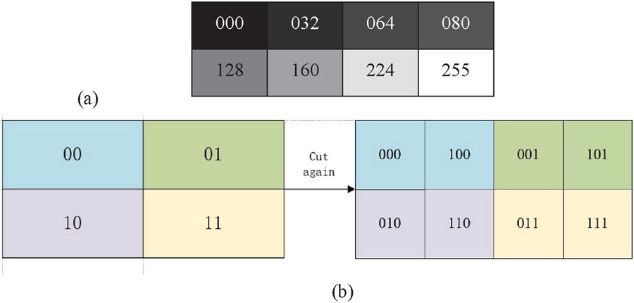
Figure 1 Example of a 2$\times$4 gray-scale image (a) Decimal representation of image gray-scale values (b) Encoding process and pixel location.

As can be seen in Figure 1(b), QBRK indicates that a $2\times 4$ image needs to be cut twice. First, the image is quadratically divided and encoded sequentially, at which point the width of the image is already in pixels and no further cuts can be made. Subsequently, the image subblocks are bisected along the direction perpendicular to the length and encoded sequentially to obtain the pixel location representation.

According to Equation (8), the storage process of the image can be obtained by combining the quantum model proposed in this paper as:

$$\{\begin{array}{ccc}\hfill |{\phi }^0⟩& \hfill =\hfill & \frac{1}{\sqrt{2^3}}(|0⟩|000⟩+|0⟩|100⟩+|0⟩|001⟩+|0⟩|101⟩\hfill \\ & & +|0⟩|010⟩+|0⟩|110⟩+|0⟩|110⟩+|1⟩|111⟩)\hfill \\ \hfill |{\phi }^4⟩& \hfill =\hfill & \frac{1}{\sqrt{2^3}}(|0⟩|000⟩+|1⟩|100⟩+|0⟩|001⟩+|1⟩|101⟩\hfill \\ & & +|0⟩|010⟩+|1⟩|110⟩+|1⟩|110⟩+|1⟩|111⟩)\hfill \\ \hfill |{\phi }^5⟩& \hfill =\hfill & \frac{1}{\sqrt{2^3}}(|0⟩|000⟩+|1⟩|100⟩+|0⟩|001⟩+|0⟩|101⟩\hfill \\ & & +|0⟩|010⟩+|1⟩|110⟩+|1⟩|110⟩+|1⟩|111⟩)\hfill \\ \hfill |{\phi }^6⟩& \hfill =\hfill & \frac{1}{\sqrt{2^3}}(|0⟩|000⟩+|0⟩|100⟩+|1⟩|001⟩+|1⟩|101⟩\hfill \\ & & +|0⟩|010⟩+|0⟩|110⟩+|1⟩|110⟩+|1⟩|111⟩)\hfill \\ \hfill |{\phi }^7⟩& \hfill =\hfill & \frac{1}{\sqrt{2^3}}(|0⟩|000⟩+|0⟩|100⟩+|0⟩|001⟩+|0⟩|101⟩\hfill \\ & & +|1⟩|010⟩+|1⟩|110⟩+|1⟩|110⟩+|1⟩|111⟩)\hfill \\ \hfill |{\phi }^1⟩& \hfill =\hfill & |{\phi }^2⟩=|{\phi }^3⟩=|{\phi }^0⟩,\hfill \end{array}$$

(8)

where $|{\phi }^l⟩$ denotes the gray-scale image information stored in the $l$ bit-plane and $l\in \{0,1,\mathrm{\dots },7\}$.

The complete information of the image is expressed as:

$$|\phi ⟩=\sum _{l=0}^7|{\phi }^l⟩|l⟩.$$

(9)

3.2 QBRK Representation for RGB Color Images

Color image can be represented as a superposition of gray-scale images on the R, G, B channels. Therefore, when representing a color image, it is sufficient to represent the gray-scale images on each of the three channels.

$$\{\begin{array}{ccc}\hfill |{\phi }^R⟩& \hfill =\hfill & \frac{1}{\sqrt{2^3}}\sum _{l=0}^7\sum _{i_{s+1},\mathrm{\dots }{i}_t=0,1}\sum _{i_1,i_2\mathrm{\dots }{i}_s=00,01,10,11}\hfill \\ & & \times |g_R(i_t,\mathrm{\dots },i_1)⟩|i_t,\mathrm{\dots }{i}_1⟩|l⟩\hfill \\ \hfill |{\phi }^G⟩& \hfill =\hfill & \frac{1}{\sqrt{2^3}}\sum _{l=0}^7\sum _{i_{s+1},\mathrm{\dots }{i}_t=0,1}\sum _{i_1,i_2\mathrm{\dots }{i}_s=00,01,10,11}\hfill \\ & & \times |g_G(i_t,\mathrm{\dots },i_1)⟩|i_t,\mathrm{\dots }{i}_1⟩|l⟩\hfill \\ \hfill |{\phi }^B⟩& \hfill =\hfill & \frac{1}{\sqrt{2^3}}\sum _{l=0}^7\sum _{i_{s+1},\mathrm{\dots }{i}_t=0,1}\sum _{i_1,i_2\mathrm{\dots }{i}_s=00,01,10,11}\hfill \\ & & \times |g_B(i_t,\mathrm{\dots },i_1)⟩|i_t,\mathrm{\dots }{i}_1⟩|l⟩,\hfill \end{array}$$

(10)

where $l\in \{0,1,\mathrm{\dots },7\}$, $|g_R(i_t,\mathrm{\dots },i_1)⟩$, $|g_G(i_t,\mathrm{\dots },i_1)⟩$, $|g_B(i_t,\mathrm{\dots },i_1)⟩\in \{0,1\}$, $|{\phi }^R⟩,|{\phi }^G⟩$, $|{\phi }^B⟩$ store the image information on each of the three RGB channels. Thus, the color image can be represented as a whole as:

$$|\phi ⟩=\frac{1}{\sqrt{3}}(|{\phi }^R⟩|01⟩+|{\phi }^G⟩|10⟩+|{\phi }^B⟩|11⟩),$$

(11)

where $|{\phi }^R⟩,|{\phi }^G⟩,|{\phi }^G⟩$ denote the image information of R, G, B channels, respectively.

Therefore, using QBRK model to represent a color image of size $2^{2n-k}\times 2^k$ requires $2n+6$ quantum qubits, where $2n$ quantum bits represent the position information of the image, 1 quantum bit represents the color information on different bit-planes, 3 quantum bits represent the bit-plane information, and 2 quantum bits represent the color channel information.

3.3 The Advantages of QBRK

Real Ket model can only represent square images, but QBRK can represent $2^{2n-k}\times 2^k$ images, increasing the range of applicability of the model. Distinguished from the traditional quantum image representation model based on NEQR model, QBRK model is improved based on the image segmentation principle of the Real Ket model. QBRK model is more proper for quantum image encryption because the quantum encoding regularity is not obvious and the position encoding of the image can be sliced.

Table 1 lists the number of quantum bits used by some quantum image representation models for encryption of $2^{2n-k}\times 2^k$ color images. It also shows that QBRK occupies fewer quantum bits, which can effectively save storage space.

Table 1 Number of quantum bits occupied by different models

Quantum Model	Number of Occupied Quantum Bits
NEQR [16]	$2n+24$
NCQI [19]	$2n+24$
BRQI [18]	$2n+6$
QRCI [19]	$2n+6$
QBRK (proposed)	$2n+6$

4 Image Encryption Algorithm Based on QBRK

An image encryption technique is put forward on the basis of the pixel position encoding and color information representation properties of QBRK model with chaotic systems and quantum bit-plane XOR operations. Figure 2 illustrates its flowchart. First, we use QBRK model to represent the original image as $|\mathrm{\Phi }⟩$. Second, we generate two matrices to perform the rank transformation on the bit-plane using a modified logistic chaos system. Third, we perform XOR operation on pixels at the same location based on the parity bit-plane, and then overlay the bit-plane for the image $|P⟩$. Finally, we use the logistic chaos system to disrupt the pixel positions for the cipher image $|C⟩$.

Figure 2 Encryption process.

4.1 Bit-plane Encryption

QBRK model distributes the color information of a gray-scale image on eight bit-planes, so that the color information on each bit-plane is either 0 or 1. In bit-plane encryption, we construct the transformation matrix using chaotic mapping, which makes the key randomized.

Step 1: For an image of $2^{2n-k}\times 2^k$, let $M=2^{2n-k}$, $N=2^k$. Use the chaotic system [20] shown in Equation (12) to generate two chaotic sequences, where the length of $y_1$ is $M\times M$, and the length of $y_2$ is $N\times N$.

$$\{\begin{array}{c}{x}_i(k_i+1)=\mu \times x_i(k_i)\times (1-x_i(k_i))\hfill \\ y_i(k_i+1)=\frac{1}{\pi }\times \arcsin (sqrt(y_i(k_i+1))),\hfill \end{array}$$

(12)

where $i\in \{1,2\}$, $k_1=0,1,2,\mathrm{\dots },M\times M$, $k_2=0,1,2,\mathrm{\dots },N\times N$, and $x_k,y_k\in \{0,1\}$.

Step 2: The two chaotic sequences obtained are mapped to integer sequences respectively by the following equation.

$$\{\begin{array}{c}p(k_1)=\mathit{round}(y_1(k_1)\times {\alpha }_1)\mathit{mod}M\hfill \\ q(k_2)=\mathit{round}(y_2(k_2)\times {\alpha }_2)\mathit{mod}N,\hfill \end{array}$$

(13)

where $k_1=0,1,2,\mathrm{\dots },M\times M$, $k_2=0,1,2,\mathrm{\dots },N\times N$, and ${\alpha }_1$, ${\alpha }_2$ are random keys larger than $M$ and $N$ respectively.

Step 3: Convert the obtained matrix $p$ and $q$ into the matrix $C_p$ and $C_q$ of bit-plane row and column transformation according to the matrix transformation rules of Equations (14) and (15) respectively.

$$C_p(x,y)=\{\begin{array}{cc}1\mathit{\hspace{1em}}\hfill & n=p(x)+1\hfill \\ 0\mathit{\hspace{1em}}\hfill & n\ne p(x)+1,\hfill \end{array}$$	(14)
$$C_q(x,y)=\{\begin{array}{cc}1\mathit{\hspace{1em}}\hfill & m=q(y)+1\hfill \\ 0\mathit{\hspace{1em}}\hfill & m\ne q(y)+1,\hfill \end{array}$$	(15)

where $x$ and $y$ are the position subscripts of the formed row and column transformation, $x\in [1,M]$, $y\in [1,N]$.

Step 4: Convert the color information on each bit-plane into a matrix $|E^i⟩$ form of size $M\times N$. Then perform row and column transformation for the eight bit-planes as shown in Equation (16).

$$|{\mathrm{\Psi }}^i⟩=C_p\times |E^i⟩\times C_q,$$

(16)

where $i\in \{0,1,\mathrm{\dots },7\}$.

Hence, the ciphertext image acquired by the first encryption $|A⟩$ can be expressed as:

$|\mathrm{A}⟩$	$={\displaystyle \frac{1}{\sqrt{2^3}}}{\displaystyle \sum _{{\mathrm{i}}_{\mathrm{s}+1},\mathrm{\dots }{\mathrm{i}}_{\mathrm{t}}=0,1}}{\displaystyle \sum _{{\mathrm{i}}_1,{\mathrm{i}}_2\mathrm{\dots }{\mathrm{i}}_{\mathrm{s}}=00,01,10,11}}{\displaystyle \sum _{\mathrm{i}=0}^7}{\mathrm{C}}_{\mathrm{p}}\times |{\mathrm{E}}^{\mathrm{i}}⟩\times {\mathrm{C}}_{\mathrm{q}}|{\mathrm{i}}_{\mathrm{t}},\mathrm{\dots }{\mathrm{i}}_1⟩|\mathrm{l}⟩,$
	$={\displaystyle \frac{1}{\sqrt{2^3}}}{\displaystyle \sum _{s,\mathrm{\dots }{i}_t=0,1}}{\displaystyle \sum _{i_1,i_2\mathrm{\dots }{i}_s=00,01,10,11}}{\displaystyle \sum _{i=0}^7}|{\mathrm{\Psi }}^i⟩|i_t,\mathrm{\dots }{i}_1⟩|l⟩.$	(17)

4.2 Parity Bit-plane Based XOR Operation

After the bit-plane encryption operation, we obtain the transformed eight bit-planes $|{\mathrm{\Psi }}^i⟩$, $i\in \{0,1,\mathrm{\dots },7\}$, and then we perform an XOR operation on the elements in the same positions of the odd and even bit-planes respectively. Next, we replace the value in the bit-plane with the smaller number with the obtained result. Finally, we change the original value in the bit-plane to the lower number. The specific operations performed are as follows.

$|{\mathrm{\Psi }}^0(x,y)⟩$	$=|{\mathrm{\Psi }}^0(x,y)⟩\oplus |{\mathrm{\Psi }}^2(x,y)⟩,$	(18)
$|{\mathrm{\Psi }}^1(x,y)⟩$	$=|{\mathrm{\Psi }}^1(x,y)⟩\oplus |{\mathrm{\Psi }}^3(x,y)⟩,$
$|{\mathrm{\Psi }}^2(x,y)⟩$	$=|{\mathrm{\Psi }}^2(x,y)⟩\oplus |{\mathrm{\Psi }}^4(x,y)⟩,$
$|{\mathrm{\Psi }}^3(x,y)⟩$	$=|{\mathrm{\Psi }}^3(x,y)⟩\oplus |{\mathrm{\Psi }}^5(x,y)⟩,$
$|{\mathrm{\Psi }}^4(x,y)⟩$	$=|{\mathrm{\Psi }}^4(x,y)⟩\oplus |{\mathrm{\Psi }}^6(x,y)⟩,$
$|{\mathrm{\Psi }}^5(x,y)⟩$	$=|{\mathrm{\Psi }}^5(x,y)⟩\oplus |{\mathrm{\Psi }}^7(x,y)⟩,$
$|{\mathrm{\Psi }}^6(x,y)⟩$	$=|{\mathrm{\Psi }}^6(x,y)⟩\oplus |{\mathrm{\Psi }}^0(x,y)⟩,$
$|{\mathrm{\Psi }}^7(x,y)⟩$	$=|{\mathrm{\Psi }}^7(x,y)⟩\oplus |{\mathrm{\Psi }}^1(x,y)⟩,$

where $(x,y)$ is the position coordinate of the pixel in the bit plane, $x\in [1,M],$ $y\in [1,N]$.

Hence, the ciphertext image acquired by the first encryption $|P⟩$ can be expressed as:

$|P⟩={\displaystyle \frac{1}{\sqrt{2^3}}}{\displaystyle \sum _{l=0}^7}{\displaystyle \sum _{i_{s+1},\mathrm{\dots }{i}_t=0,1}}{\displaystyle \sum _{i_1,i_2\mathrm{\dots }{i}_s=00,01,10,11}}|{\mathrm{\Psi }}^i⟩|i_t,\mathrm{\dots }{i}_1⟩|l⟩.$

(19)

Due to the self-reflexive nature of the heterogeneous operation itself, while $c=a\oplus b$, $a\oplus b\oplus a=c\oplus a=b$. Therefore, in the decryption process, we use a stepwise decryption starting from $|{\mathrm{\Psi }}^6⟩$ and $|{\mathrm{\Psi }}^7⟩$.

4.3 Pixel Position Information Encryption

After changing the color of the pixel, we designed the following operation to change the position of the pixel. With the discussion in Section 3, the encryption of a $2^{2n-k}\times 2^k$ quantum image using the present model requires cutting $t=\mathit{max}\{2n-k,k\}$ times. Therefore, according to the logical map [21], we generate a chaotic sequence with a length of $t$, and establish a map of the sequence and the position coding obtained by each cut of the pixel. Then, the chaotic sequence is sorted to disrupt the pixel position coding. Finally, the new position code is converted to octal, and all pixels in the image are sorted.

Step 1: Generate a chaotic sequence [21] of length $t$ by

$$x_{k+1}=\mu \times x_k\times (1-x_k),$$

(20)

where $k=0,1,2,\mathrm{\dots },t$ and $x_k\in \{0,1\}$.

Step 2: Establish a map of the sequence and the position coding obtained by each cut of the pixel. The specific mapping relationship is shown in Equation (21).

$$|i_t,\mathrm{\dots }{i}_1⟩=\{\begin{array}{cc}\mathit{First}\mathit{cut}:|i_1⟩\mathit{\hspace{1em}}\hfill & ⟶x_t\hfill \\ \mathit{Second}\mathit{cut}:|i_2⟩\mathit{\hspace{1em}}\hfill & ⟶x_{t-1}\hfill \\ \multicolumn{2}{c}{\mathrm{\dots }}\\ \mathit{The}t-\mathit{th}\mathit{cut}:|i_t⟩\mathit{\hspace{1em}}\hfill & ⟶x_1,\hfill \end{array}$$

(21)

Step 3: The chaotic sequences are compared in order of size, if $x_k$ is smaller than $x_{k+1}$, the position information corresponding to $x_k$ and $x_{k+1}$ is not changed; conversely, if $x_k$ is larger than $x_{k+1}$, the position information corresponding to $x_k$ and $x_{k+1}$ is exchanged.

Convert the position information of pixels into octal representation to sort from small to large, and we can get the encrypted image $|C⟩$ by:

$|C_{2^{2n-k}\times 2^k}⟩$	$={\displaystyle \frac{1}{\sqrt{2^3}}}{\displaystyle \sum _{i_{s+1},\mathrm{\dots }{i}_t=0,1}}{\displaystyle \sum _{i_1,i_2\mathrm{\dots }{i}_s=00,01,10,11}}{\displaystyle \sum _{i=0}^7}$
	$\mathrm{\hspace{1em}}\times |g(i_t,\mathrm{\dots },i_1)⟩|i_t,\mathrm{\dots }{i}_1⟩|l⟩,$	(22)

where $i_k,\mathrm{\dots }{i}_1$ is the pixel position sequence obtained after encryption.

Take an image of $2^2\times 2^3$ as an example, we chose $\mu =4$, and $x_0=0.78$. Then we can get a chaotic sequence of length 3.

$$\mathit{sequence}:\mathrm{\hspace{0.25em}0.78}\mathit{\hspace{1em}}0.6864\mathit{\hspace{1em}}0.8610.$$

(23)

According to the rules defined above, we this results in the encryption process of the image as shown in Figure 3.

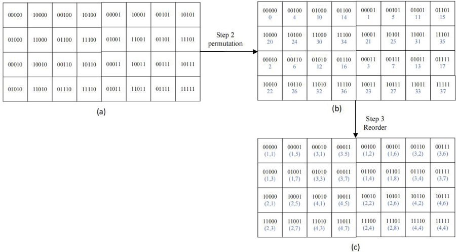
Figure 3 Example of image encryption process.

Figure 3(a) shows the initial position encoding of every pixel of the image. For a $2^2\times 2^3$ image, the image needs to be cut 3 times to get the encoding of the image. By sorting the chaotic sequence, we exchange the code of the corresponding third segment with the code of the second segment. Figure 3(b) illustrates the position encoding of the disordered pixels, and the blue part indicates the corresponding octal number. Figure 3(c) presents the result after sorting by octal number size, and the blue part indicates where the pixel at that position is located in Figure 3(a). Figure 3 displays that the chaotic sequence is extremely short, only one cut position exchange is experienced to achieve the effect that all pixels outside of $(1,1)$ and $(4,4)$ have completed the position transformation. For a $512\times 512$ image, we need to generate a logistic chaos sequence of length 8 for dislocation, which can produce a better dislocation effect and complete the operation of pixel diffusion.

Take the pixel at position $(3,4)$ as an example, it needs to go through three cuts to get the complete pixel code. In the first cut, it belongs to the third part with position code $|10⟩$; in the second cut, it belongs to the second part with position code $|01⟩$; in the third cut, it belongs to the second part with position code $|1⟩$. Therefore, the initial position code of $(3,4)$ is $|10110⟩$. Subsequently, the pixel position code is scrambled and the position code of $(3,4)$ becomes $|01110⟩$. Finally, the octal representation of the position code is sorted, and the initial pixel $(3,4)$ is converted to the position of $(2,7)$.

5 Image Simulation Results and Complexity Analysis

For testing purposes the encryption and decryption roles of the proposed algorithm, Intel(R) Core(TM) i5-10300H CPU @ 2.50 GHz processor, Windows 10, 64-bit operating system are used in Matlab 2018b for simulation experimental processing. In the simulation experiments, we set the keys as ${\mu }_1=4$, ${\mu }_2=4$, ${\alpha }_1=1015$, ${\alpha }_2=1015$, $x_1(1)=0.78$, $x_2(1)=0.32$, $\mathit{sum}A=\mathit{Sum}\mathit{of}\mathit{the}\mathit{pixel}\mathit{grayscale}\mathit{values}\mathit{of}\mathit{the}\mathit{channels}.$

We choose the color image “Lena” and grayscale image “Peppers” of both size $512\times 512$ for simulation experiments. Figure 4 presents the original, ciphertext and plaintext images obtained after decryption. It must be noted that we can see no difference between the decrypted and the original images with the naked eye, and we cannot get any information of the original image visually from the ciphertext image.

Figure 4 Simulation experiment results figures (a)–(c) are the original image, encrypted image, and decrypted image of ‘Lena’ image in order; (d)–(f) are the original image, encrypted image, and decrypted image of ‘Peppers’ image in order.

5.1 Histogram Analysis

In this subsection, in order to count the distribution of gray-scale levels in the image to check the role of encryption, we put the image to a gray-scale histogram analysis. Figure 5 illustrates the histograms of the three signal channels for the ‘Lena’ plaintext and ciphertext color images as well as the histogram for the ‘Peppers’ in gray-scale image. The illustration shows how much more uniform the histogram information is for the ciphertext image than it is for the plaintext image. As a result, it can be concluded that the plaintext image cannot be immediately inferred from the ciphertext image acquired.

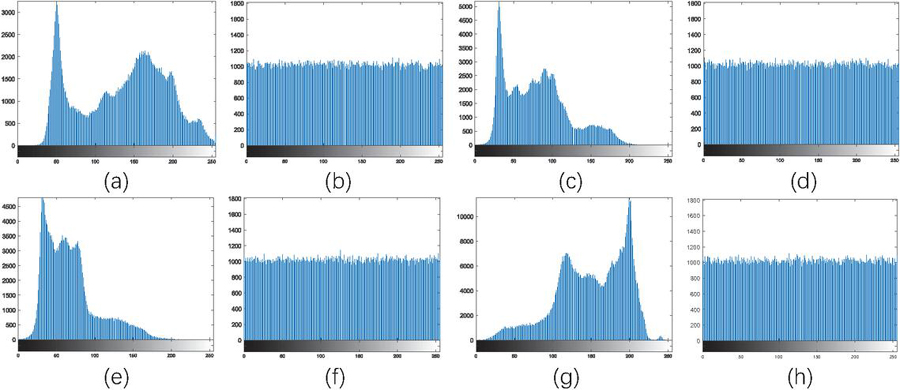
Figure 5 The histograms of the three signal channels for ‘Lena’ and ‘Peppers’ (a), (c), (e) represent the gray-scale scale histogram of RGB channel of ‘Lena’ image; (b), (d), (f) represent the gray-scale scale histogram of RGB channel of ciphertext image; (g) (h) represent the gray-scale scale histogram of ‘Peppers’ image and its ciphertext image.

5.2 Time Complexity Analysis

As we know, time complexity is also an important index for image encryption algorithm, for an image of $2^{2n-k}\times 2^k$, let $t=\mathit{max}\{2n-k,k\}$, there are three parts that take up more time in the process of image encryption. The first part is pixel position replacement, which mainly includes image cutting, representation of pixel positions and generation of chaotic sequences, and its time complexity is $O(t)=\max \{O(1),O(t)\}$. The second part is the pixel color perturbation part, which mainly includes the operations of perturbation matrix generation and pixel permutation, and its time complexity is $O(t^2)$; the third part is the pixel diffusion operation, which mainly includes the quantum $\mathit{CNOT}$ gate operation in the bit-plane, and its time complexity is $O(1)$.

The speed of image encryption is one of the important indicators of image encryption algorithms. For better test the proposed algorithm, we need to compare the encryption and decryption times of color images with those in [22], which was proposed in 2022 and applied XOR operations similar to this article for encryption. We also compare the encryption and decryption times of different images using an improved chaotic system. Table 2 presents the comparison outcomes. From the data in the table, we can see that the encryption and decryption time of the proposed algorithm for three classic images is shorter than that in [22]. At the same time, due to the improved algorithm based on chaotic sequences and the introduction of XOR, cutting and other operations, the encryption and decryption time of QBRK is longer than that of chaotic systems. Therefore, it can be concluded that the model and the algorithm encrypt in a shorter time and may have better application prospects.

Table 2 Algorithm encryption and decryption time

	Image	QBRK(s)	Chaotic Mapping(s)	Ref. [22](s)
	Lena	7.35	0.93	19.14
Encryption	Pepper	7.05	0.90	19.97
	Baboon	7.45	0.86	21.50
	Lena	7.49	0.74	20.93
Decryption	Pepper	7.36	0.74	19.91
	Baboon	7.84	0.72	21.22

6 Security Analysis

Since ciphertext pictures could be attacked by outsiders during image transmission, their security is a crucial sign of the effectiveness of image encryption techniques. We analyze the ciphertext image thoroughly and evaluates the proposed algorithm using a variety of ways.

6.1 Correlation Analysis of Adjacent Pixels

There is a clear correlation between adjacent pixels of the images. The correlation between neighboring pixels of the ciphertext image is very strong, if we want to make the data of the ciphertext image inaccessible to the attacker directly, we should minimize the correlation between neighboring pixels in all directions of the ciphertext image, including horizontal, vertical and diagonal directions. We randomly select K $=$ 30000 pairs of adjacent pixels to detect the adjacent pixel correlation of plaintext and ciphertext images.

We chose the color “Lena” image as an instance to detect the correlation of adjacent pixels in different channels in horizontal, vertical and diagonal directions. Figure 6 shows the correlation of 30,000 pairs of adjacent pixels in the R, G and B channels of plaintext and ciphertext images in the horizontal, vertical, and diagonal directions. The blue scatter, green scatter and red scatter in the figure indicate the correlation between adjacent pixels of R channel, G channel and B channel, respectively. It is obvious from Figure 6 that the adjacent pixels of every channel of the original “Lena” image show strong correlation and linearity in all directions, while the adjacent pixels in the ciphertext image are highly scattered and disordered, which means the correlation between adjacent pixels is extremely weak. It can be concluded that attackers cannot directly obtain the valid information from the ciphertext image.

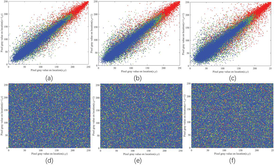
Figure 6 Correlation coefficient of adjacent pixels (a) ‘Lena’ horizontal direction (b) ‘Lena’ vertical direction (c) ‘Lena’ diagonal direction (d) Cipher horizontal direction (e) Cipher vertical direction (f) Cipher diagonal direction.

Moreover, the correlation coefficient is used to show the relationship between neighboring pixels more visually. The correlation coefficient is calculated as in Equation (24).

$$r_{\mathit{xy}}=\frac{\mathit{cov}(x,y)}{\sqrt{D(x)}\sqrt{D(y)}},$$

(24)

where $x$ and $y$ are the positions of a pair of adjacent pixels, $\mathit{cov}(x,y)$ means the covariance of $x$ and $y$, $D(x)$ stands for the variance, $r_{xy}\in \{-1,\mathrm{\hspace{0.25em}1}\}$, and $|r_{xy}|$ the smaller, the lower the correlation between adjacent pixels.

The correlation coefficients of adjacent pixels in every direction of the ‘Lena’ image are listed in Table 3. The obtained results prove that the correlation coefficient of the plaintext image is close to 1, that is, the correlation between adjacent pixels of a plaintext image is strong. While the correlation coefficient of the ciphertext image is close to 0, that is, no significant correlation between adjacent pixels is found. While comparing the data in Refs. [23, 25] and the improved logistic chaotic mapping, the correlation coefficients of adjacent pixels in the nine directions of the proposed algorithm are only higher in one direction than in [23], slightly higher in only two directions than [25], and lower in all directions than the chaotic mapping. This means that the proposed algorithm has lower correlation coefficients of adjacent pixels in more directions. And this advantage does not solely rely on encryption with chaotic mapping. Therefore, attackers cannot decipher ciphertext images through statistical analysis and correlation analysis.

Table 3 Correlation coefficients of adjacent pixels in various directions for color ‘Lena’ image

						Chaotic
Channel	Direction	Plain Image	QBRK	Ref. [23]	Ref. [25]	Mapping
	Horizontal	0.98378886	0.00091612	0.0071	-0.001854	0.0069
R	Vertical	0.97105290	0.00181037	0.0418	-0.021045	-0.0113
	Diagonal	0.95833005	0.00257735	0.0092	0.0070670	0.0142
	Horizontal	0.97825353	0.00117159	-0.0039	-0.029268	-0.0136
G	Vertical	0.96197501	0.00223737	-0.00009	0.0012360	0.0159
	Diagonal	0.94658953	0.00304897	-0.0034	-0.09406	0.0065
	Horizontal	0.96651105	-0.0066649	0.0014	-0.005394	0.0108
B	Vertical	0.94267581	0.00058526	0.0061	0.050137	-0.0319
	Diagonal	0.92037511	-0.0012418	-0.0128	0.0019080	0.0073

6.2 Information Entropy Analysis

Information entropy analysis is a significant index to test image encryption algorithms. The formula for calculating the information entropy is shown below.

$$H(X)=-\sum _{i=1}^{n}p(x_i)lo{g}_{2}p(x_i),$$

(25)

where $n$ denotes the gray-scale level of the image, and all the images used in this paper have $n=256$, and $p(x_i)$ means the possibility of occurrence of the gray-scale value $x_i$. Since the color range of each channel of the image is within $[0,2^8-1]$, the theoretical value of $H(X)$ is 8.

We take a 512 $\times$ 512 color ‘Lena’ image as an example and perform information entropy analysis for R, G and B channels, and compare the results with those in Refs. [24–26] and the improved logistic chaotic mapping. We list all the data in Table 4. From the table, the data entropy of the plaintext image is significantly smaller than that of the ciphertext image. And the average value of the information entropy of each channel of the ciphertext image reaches 7.99933, all of which are higher than those in Refs. [24–26] and chaotic mapping, so it can be concluded that the ciphertext image acquired by the proposed algorithm has a higher confusion degree and can better resist the information entropy attack.

Table 4 Information entropy of ‘Lena’ images on different channels

Channel	Plain Image	QBRK	Ref. [24]	Ref. [26]	Ref. [25]	Chaotic Mapping
R	7.3388	7.9993	7.9938	7.9974	7.999281	7.9911
G	7.4963	7.9993	7.9951	7.9976	7.999337	7.9912
B	7.0583	7.9994	7.9952	7.9974	7.999335	7.9911
Average	7.2978	7.99933	7.9947	7.9975	7.999318	7.99113

6.3 Key Sensitivity Analysis

A good encryption algorithm must exhibit a high sensitivity to the key, which can be changed by a very small amount and still have a huge impact on encryption and decryption. We set seven keys to decrypt the cipher image which are ${\mu }_1$, ${\mu }_2$, ${\alpha }_1$, ${\alpha }_2$, $x_1(1)$, $x_2(1)$, $\mathit{sumA}$. ${\mu }_1$ and ${\mu }_2$ are used to control the degree of chaos of the logistic chaotic sequence. It has been shown that the chaotic state is optimal when ${\mu }_1={\mu }_2=4$ [21], so we do not discuss the sensitivity of ${\mu }_1$ and ${\mu }_2$. The color ‘Lena’ image is taken as an example, and the six images shown in Figure 7 are obtained by making small changes to each of the remaining five keys. From this figure we can observe that the correct plain image cannot be obtained even with the key with small differences, and the decrypted image with the wrong key cannot visualize any valid information. Therefore, we can assume that the keys used by the proposed algorithm are highly sensitive.

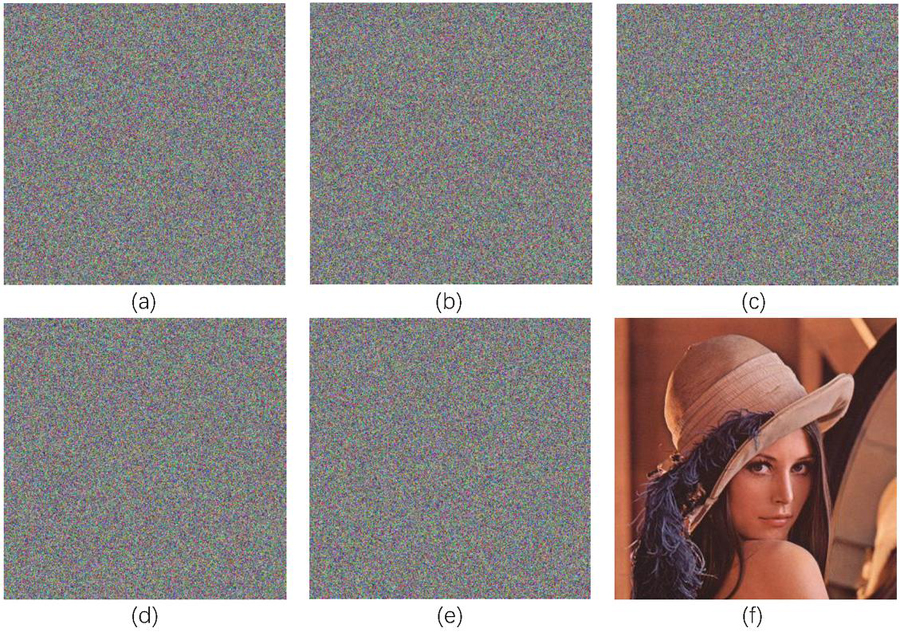
Figure 7 Minimally changing the key for decryption (a) $x_1(1)+{10}^{-16}$ (b) $x_2(1)+{10}^{-16}$ (c) ${\alpha }_1+1$ (d) ${\alpha }_2+1$ (e) $\mathit{sum}A+10$ (f) Correct key.

6.4 Differential Attack Analysis

Differential analysis is a selective plaintext attack [27] that can effectively judge the encryption effectiveness of the algorithm. When a pixel value of the plaintext image is changed, the ciphertext image will be changed substantially. We chose two metrics to evaluate the resistance of the algorithm to differential attacks. The first metric is the pixel change rate ($\mathit{NPCR}$) it represents the number of pixel variations between two encrypted images. The second metric is the Uniform Average Change Intensity ($\mathit{UACI}$) which is used to calculate the mean number of changes in intensity between two encrypted images. They are calculated as follows.

$\mathit{NPCR}$	$={\displaystyle \frac{{\sum }_{i=1}^M{\sum }_{j=1}^{N}D(i,j)}{M\times N}}\times 100\%,$	(26)
$\mathit{UACI}$	$={\displaystyle \frac{1}{M\times N}}{\displaystyle \sum _{i=1}^M}{\displaystyle \sum _{j=1}^N}{\displaystyle \frac{|I_1(i,j)-I_2(i,j)|}{255}}\times 100\%,$	(27)

where $I_1$, $I_2$ are ciphertext images, which are obtained by encrypting the original image and the plaintext image modified by one pixel, respectively, and $D(i,j)=0$ when $I_1(i,j)=I_2(i,j)$, otherwise $D(i,j)=1$. We use three different images as examples to test the algorithm’s resistance to differential attacks and compare the results with the corresponding images in Refs. [22, 26] and chaotic mapping. Table 5 shows $\mathit{NPCR}$ and $\mathit{UACI}$ values. The ideal value of $\mathit{NPCR}$ and $\mathit{UACI}$ are 99.6094% and 33.4635%.

Results presented in Table 5 proves that $\mathit{NPCR}$ and $\mathit{UACI}$ obtained by changing a pixel value in each channel are close to the ideal values. Comparing with the literatures and chaotic mapping, the proposed algorithm has better results in both $\mathit{NPCR}$ and $\mathit{UACI}$. Therefore, it can be considered that the proposed algorithm has better resistance to differential attacks.

Table 5 NPCR and UACI of the images

	NPCR [%]			UACI [%]
Image	R	G	B	R	G	B
Lena	99.6162	99.6116	99.6054	33.5057	33.4224	33.4735
Peppers	99.6091	99.6130	99.6140	33.4315	33.4273	33.4894
Baboon	99.6114	99.6071	99.6063	33.4694	33.4752	33.4224
Ref. [22] in Lena	99.6535	99.5770	99.6560	33.4943	33.5117	33.5901
Ref. [25] in Lena	99.6037	99.5983	99.6159	33.4290	33.4306	33.3665
Ref. [26] in Baboon	99.6185	99.6075	99.6143	33.4766	33.4968	33.4689
Chaotic mapping in Lena	99.6136	99.6225	99.5979	33.5451	33.5846	33.6196
Chaotic mapping in Peppers	99.6323	99.6323	99.5998	33.5974	33.4359	33.7761

6.5 Cropping Attack

Images may lose some data due to external attacks during transmission. To detect the robustness of image against cropping attack. Taking a $512\times 512$ color ‘Lena’ image as an example, we do $100\times 100$ edge cropping attack, $212\times 212$ and $256\times 512$ center cropping attack on the ciphertext image respectively. Figure 8 shows the attacked ciphertext images and the corresponding plaintext images. Figure 8(e)–(h) displays that the pixels of the decrypted image are affected to different degrees, but the main feature information of the original image is still retained. As the cropping continues to expand, the more image information is lost in the decrypted image. However, the cipher text image obtained by the proposed algorithm does not affect the main image features of the decrypted image even if 50% of the image data information is lost. Hence, it is concluded that the proposed algorithm can resist cropping attacks and has good robustness against cropping.

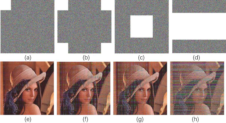
Figure 8 Crop attack (a) ciphertext image with one $100\times 100$ edge crop; (b) ciphertext image with four $100\times 100$ edge crops; (c) ciphertext image with $212\times 212$ center crop; (d) ciphertext image with $256\times 512$ horizontal crop; (e)-(h) decrypted images corresponding to the image above them.

6.6 Noise Attack

Images may suffer from different noise attacks during transmission, such as Gaussian noise, pretzel noise, Poisson noise, etc. For detecting the anti-noise robustness of ciphertext images, we design the anti-noise experiments on ciphertext images to verify the stability of the encryption algorithm. We take the color “Lena” image as an instance and add pepper noise with densities of 0.01, 0.03 and 0.1 to the ciphertext image. Then we decrypt the image with added noise for testing, and the obtained plaintext image is filtered with $3\times 3$, $5\times 5$, and $7\times 7$ median for noise removal, and Figure 9 displays the obtained outcomes.

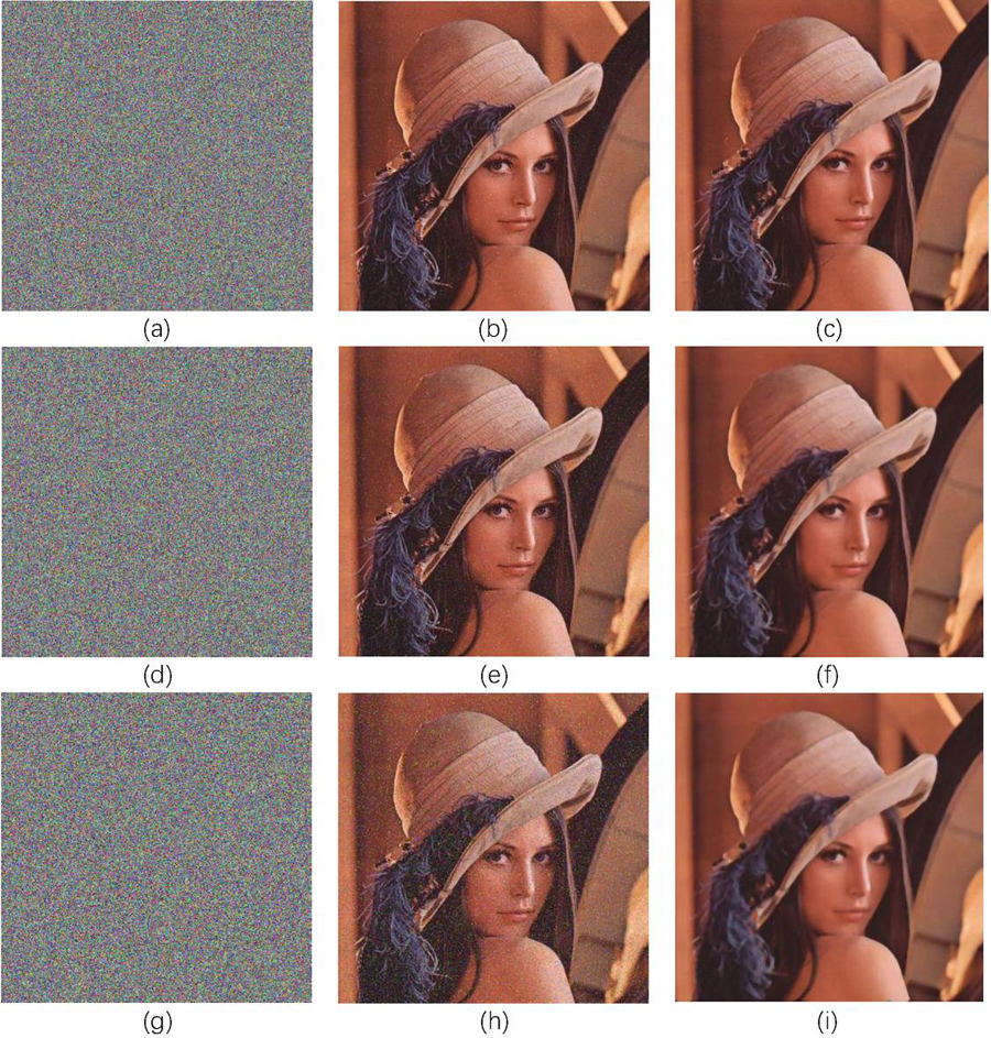
Figure 9 (a), (d), (g) represent the ciphertext images with the addition of pretzel noise of intensity 0.01, 0.03, 0.1, respectively; (b), (e), (h) represent the corresponding decrypted images; (c), (f), (i) represent the images after noise removal, respectively.

Figure 9 illustrates that with the increase in the density of the pretzel noise, the decrypted image loses gradually more image information, but the naked eye can still identify the main features of the image. As the two-dimensional sliding template of median filtering gradually increases, the higher the blurring of the restored image obtained, that is, the worse the elimination effect for isolated noise points. However, it can still be considered that the peppers of different densities can be separated from the reduced image, that is, the image has good anti-noise robustness.

7 Conclusions

This paper puts forward a quantum bit-plane representation of the Real Ket model (QBRK). The model implements the quantization of the Real-Ket model and extends the application to rectangular images of $2^{2n-k}\times 2^k$. In addition, the model is also applicable to grayscale and color images. On the basis of the QBRK model and chaotic system, an image encryption algorithm is proposed that relies on pixel position encoding for slice dislocation and quantum bit-plane XOR operation. Experimental results of simulations prove that the QBRK-based image encryption algorithm has low complexity, high security, and resistance to typical image attacks. At the same time, we have also demonstrated through experiments that the advantages of the proposed algorithm do not solely depend on the improved chaotic mapping.

Funding: This research was funded by the National Students Innovation and Entrepreneurship Training Program (No. 220033).

Conflict Statement: The authors declare no conflict of interest.

References

[1] Akhshani A, Akhavan A, Lim S C. An image encryption scheme based on quantum logistic map [J]. Communications in Nonlinear Science and Numerical Simulation, 2012, 17(12): 4653–4661.

[2] Lu D J, He W Q, Peng X. Optical image encryption based on a radial shearing interferometer [J]. Journal of Optics, 2013, 15(10): 105405.

[3] Shi Y S, Li T, Wang Y L, et al. Optical image encryption via ptychography [J]. Optics Letters, 2013, 38(9): 1425–1427.

[4] Sun M J, Shi J H, Li H, et al. A simple optical encryption based on shape merging technique in periodic direction correlation imaging [J]. Optics Express, 2013, 21(16): 19395–19400.

[5] Gao, X., Mou, J., Xiong, L., Sha, Y., Yan, H., Cao, Y. A fast and efficient multiple images encryption based on single-channel encryption and chaotic system. Nonlinear Dynamics 2022, 108, 613–636.

[6] Ben Farah, M.A., Guesmi, R., Kachouri, A., Samet, M. A novel chaos based optical image encryption using fractional Fourier transform and DNA sequence operation. Optics And Laser Technology 2020, 121.

[7] Murillo-Escobar, M.A., Cruz-Hernandez, C., Abundiz-Perez, F., Lopez-Gutierrez, R.M., Acosta Del Campo, O.R. A RGB image encryption algorithm based on total plain image characteristics and chaos. Signal Processing 2015, 109, 119–131. 155.

[8] Gong, L., Qiu, K., Deng, C., Zhou, N. An image compression and encryption algorithm based on chaotic system and compressive sensing. Optics And Laser Technology 2019, 115, 25.

[9] Latorre J I. Image compression and entanglement[J]. Computer Science, 2005.

[10] Venegas-Andraca, S. Bose E. Storing, processing, and retrieving an image using quantum mechanics[C]. Proceedings of the SPIE Conference on Quantum Information and Computation, Orlando, 2003, 137–147.

[11] Venegas-Andraca, S. E, Bose S. Quantum computation and image processing: new trends in artificial intelligence[C]. Proceedings of the International Congress on Artificial Intelligence, Acapulco, Mexico, 2003, 1563–1564.

[12] J Fridrich. Symmetric ciphers based on two-dimensional chaotic maps. International Journal Of Bifurcation And Chaos, 8(6):1259–1284, Jun 1998.

[13] Chengqing Li, David Arroyo, and Kwok-Tung Lo. Breaking a chaotic cryptographic scheme based on com-position maps. International Journal Of Bifurcation And Chaos, 20(8):2561–2568, Aug 2010.

[14] Xingyuan Wang, Chuanming Liu, Dahai Xu, and Chongxin Liu. Image encryption scheme using chaos and simulated annealing algorithm. Nonlinear Dynamics, 84(3):1417–1429, May, 2016.

[15] Le P Q, Dong F Y, Hirota K. A flexible representation of quantum images for polynomial preparation image compression and processing operations [J]. Quantum Information Processing, 2011, 10(1): 63–84.

[16] Zhang Y, Lu K, Gao Y H, et al. NEQR: A novel enhanced quantum representation of digital images [J]. Quantum Information Processing, 2013, 12(8): 2833–2860.

[17] Sun B, Le P. Q, liyasu A. M., et al. A multi-channel representation for images on quantum computers using the RGB$\alpha$ color space[C]. Intelligent Signal Processing (WISP), 2011 IEEE 7th International Symposium on. IEEE, 2011: 1–6.

[18] Li, H.S., Chen, X., Xia, H., Liang, Y., Zhou, Z. A Quantum Image Representation Based on Bitplanes. IEEE Access 2018, 6, 62396–62404.

[19] Wang Ling Research on quantum representation and encryption algorithm of color digital image [D] Heilongjiang: Harbin University of Technology, 2020.

[20] A. Akhshani, A. Akhavan, S. C. Lim, and Z. Hassan, An image encryption scheme based on quantum logistic map. Communications In Nonlinear Science And Numerical Simulation 2012, 17, 4653–4661.

[21] Akhshani, A., Akhavan, A., Lim, S.C., Hassan, Z. An image encryption scheme based on quantum logistic map. Communications In Nonlinear Science And Numerical Simulation 2012, 17, 4653–4661.

[22] X. Wang, Y. Su, C. Luo, F. Nian, and L. Teng, Color image encryption algorithm based on hyperchaotic system and improved quantum revolving gate. Multimedia Tools And Applications 2022, 81, 13845–13865.

[23] Lu Aiping Li Panchi Quantum Encryption Scheme for Color Images Based on Chaotic Sequences, 2021, 49(4): 692–697730. DOI: 10.3969/j.issn.1672-9722.2021.04.017.

[24] Khorrampanah, M., Houshmand, M., Heravi, M.M.L. New method to encrypt RGB images using quantum computing. Optical And Quantum Electronics 2022, 54.

[25] Qin, X., Liu, C. Color image encryption algorithm based on customized globally coupled map lattices. Multimedia Tools And Applications 2019, 78, 6191–6209.

[26] Hosny, K.M., Kamal, S.T., Darwish, M.M. A color image encryption technique using block scrambling and chaos. Multimedia Tools And Applications 2022, 81, 505–525. 3.

[27] Wang XY, Gao S (2020) Image encryption algorithm based on the matrix semi-tensor product with a compound secret key produced by a Boolean network. Inf Sci 539: 195–214.

Biographies

Xv Zhou is currently pursuing a bachelor’s degree in Mathematics at the School of Science, Northeastern University of China. Her current research areas include chaotic systems and quantum image encryption.

Jinwen He is currently pursuing the Bachelor’s degree with the Department of Mathematics, College of Science, Northeastern University, Shenyang, China. Her current research interests include chaotic theory, chaos-based applications, and quantum image encryption.

Journal of Cyber Security and Mobility, Vol. 12_5, 757–784.
doi: 10.13052/jcsm2245-1439.1257
© 2023 River Publishers

Abstract

1 Introduction

2 Real Ket and BRQI Models

2.1 Real Ket Model

2.2 BRQI Model

3 The Proposed Model – QBRK

3.1 QBRK Representation for Gray-scale Image

3.2 QBRK Representation for RGB Color Images

3.3 The Advantages of QBRK

4 Image Encryption Algorithm Based on QBRK

4.1 Bit-plane Encryption

4.2 Parity Bit-plane Based XOR Operation

4.3 Pixel Position Information Encryption

5 Image Simulation Results and Complexity Analysis

5.1 Histogram Analysis

5.2 Time Complexity Analysis

6 Security Analysis

6.1 Correlation Analysis of Adjacent Pixels

6.2 Information Entropy Analysis

6.3 Key Sensitivity Analysis

6.4 Differential Attack Analysis

6.5 Cropping Attack

6.6 Noise Attack

7 Conclusions

References

Biographies