The Homology Determination System for APT Samples Based on Gene Maps
Rui-chao Xu1, Yue-bin Di1, Zeng Shou1, Xiao Ma2, 3, He-qiu Chai4 and Long Yin4,*
1State Grid Liaoning Electric Power Supply Co., Ltd., Shenyang 110003, China
2NARI Group Corporation (State Grid Electronic Power Research Institute), Nanjing 210061, China
3Beijing Kedong Electric Power Control System Co., Ltd., Beijing 100192, China
4Software College, Northeastern University, Shenyang 110169, China
E-mail: 2110499@stu.neu.edu.cn
*Corresponding Author
Received 28 November 2023; Accepted 21 March 2024
Abstract
At present, there are fewer types of homology determination methods for advanced persistent threat (APT) samples detection, and most existing determination schemes have problems such as high cost, low accuracy, and difficulty in identifying unknown APT samples. Therefore, we proposed a homology determination system for APT samples based on gene maps by integrating deep learning and gene maps. Firstly, we extract the software gene features from the samples uploaded by the user and apply the TF-IDF algorithm to clean the extracted software genes. The Word2Vec algorithm is used to vectorize all the genes to construct the gene sample vectors. And we use a LSTM-based classifier to detect APT attack samples. Finally, the K-nearest neighbor algorithm is used to determine the homology of gene-sharing APT samples. The detailed construction process of the scheme is given in this paper, including APT sample gene extraction, cleaning, clustering, sample detection, and homology determination. Experimental validation showcases our model outperforming existing methodologies with an accuracy of 95%, precision of 94%, and recall of 95%. When compared to previous models, the superiority of our approach is evident. These results underscore our model’s high efficiency and accuracy, confirming its potential for significant application in the field of cybersecurity.
Keywords: APT sample, gene map, homology determination.
1 Introduction
Advanced persistent threat (APT) is a type of attack that uses highly stealthy, organized, and threatening attack methods to carry out persistent cyber attacks against a specified target. Among all types of cyber attacks, APT attacks have the highest threat level and are more difficult to detect [1–3]. In 2009, a large-scale APT attack dubbed Operation Aurora targeted multiple high-profile companies, including Google, Adobe Systems, and Rackspace. The aim was to harvest sensitive corporate data and user account information. In 2010, a cyber weapon known as Stuxnet targeted Iranian nuclear facilities. The malware is a sophisticated worm that was designed to infiltrate and compromise industrial systems, specifically the Siemens SIMATIC WinCC/PCS 7 control systems used in Iran’s nuclear program. Stuxnet reportedly damaged or destroyed approximately 1,000 centrifuges. Another notable example is the 2016 U.S. Democratic National Committee (DNC) hack, where APT28 (Fancy Bear) and APT29 (Cozy Bear) were involved in stealing sensitive data, internal communications, and emails. According to QiAnXin’s Global Advanced Persistent Threat (APT) 2021 Annual Report [4], a large number of IP addresses within China have generated high-risk communications with dozens of offshore APT groups in 2021, and their number and damage are growing at an alarming rate. APT attacks on government departments, health and medical sectors, and high-tech enterprises in China are prominent.
Facing the explosive growth of APT attacks, APT detection and traceability research has received increasing attention. Although many universities, research institutes, and enterprise organizations have proposed various measures to address the problem, new types of APT attacks have emerged, and the emergence of packing, obfuscation, sandbox evasion, and other technologies have made traditional detection methods face serious challenges, and it has become unrealistic and inefficient to rely solely on manual work to identify and classify malicious code samples. Motivated by this situation, we focus on explore the deep-rooted patterns and features of APT codes and to analyse and detect unknown APT samples efficiently and accurately using machine learning, deep learning, and other related technologies. The main contributions of our study are listed as follows.
(1) We employ a multi-faceted approach that integrates TF-IDF for feature reduction, word2vec for vector construction, a three-layers LSTM module for sequential data handling, and KNN for homology determination.
(2) The proposed method can efficiently process large datasets, flexibly adapt to APT evolution, and maintain a high classification accuracy with less reliance on labeled data.
(3) Experimental validation showcases our model outperforming existing methodologies with an accuracy of 95%, precision of 94%, and recall of 95%, which proves the superiority of our approach by comparing with other APT codes detection approaches.
2 Related Works
The analysis and classification of malicious software, particularly Advanced Persistent Threats (APTs), have been extensively studied, with methodologies evolving from statistical analysis to sophisticated machine learning and deep learning techniques. This section provides a systematic review of the progression of these methodologies and highlights our novel contributions to the field. Early approaches to APT analysis focused on feature extraction through statistical methods. For instance, researchers decomposed APT source code post-decompilation and categorized features into different levels of granularity [5]. They utilized Term Frequency (TF) to prioritize APIs, illustrating the importance of feature selection in classification tasks. However, the dataset used in these studies, which will be described comprehensively in Section 5.1, is often limited in scope, and our work aims to address this by incorporating a more diverse and extensive collection of APT samples.
Graph-based analyses, such as downloader graphs and functional dependency graphs, have been employed to distinguish between benign and malicious code, with Kwon et al. [6] and Garbervetsky et al. [7] using these to analyze download patterns and function call dependencies, respectively. However, the dynamic nature of APTs poses challenges, as mutations can alter structural patterns. Our research introduces a novel gene mapping technique that enhances the robustness of graph-based methods against these APT mutations. In the realm of machine learning for APT classification, Rosenberg et al. [8] showed the determination of homology, while Pascanu et al. [9] and Miller et al. [10] used recurrent neural networks and SVM classifiers. These methods often rely on extensive labeled data, a requirement our approach reduces by applying the K-Nearest Neighbors (KNN) algorithm, allowing for effective classification with fewer labeled samples. Adding to the graph-based analysis landscape, Huang et al. [11] proposed a multi-granularity fusion feature based on biological gene concepts for binary code traceability. Similarly, Zhao et al. [12] introduced a malware homology identification method using subgraphs of the Function Dependence Graph (FDG) as genes. While insightful, these methods have limitations, such as the complexity of selecting key APIs and scalability issues. Moreover, the structural changes from malware mutations and the computational demands of FDGs pose significant challenges. Our approach aims to address these limitations, offering a scalable solution less prone to the overfitting risks associated with previous methods when analyzing new APT samples.
Deep learning has brought significant advancements in APT classification. Zhao et al. proposed a texture fingerprint-based clustering method to analyse the homology of malicious code [13]. The method analyses binary malicious programs without source code analyses their image texture fingerprint information and clusters their fingerprint information. Sun et al. proposed a malware feature images generation method combining malicious code analysis, RNN and CNN to identify malware families [14]. Zhang et al. proposed a DNN architecture applying multiple Gated-CNNs to extract features of API calls and execute dynamic malware analysis [15]. Li et al. proposed a malware classification model with RNN to classify variants of malware by using long-sequences of API calls [16]. Chaganti et al. proposed a DL based Bi-GRU-CNN model to detect the IoT malware and classify the malware families using ELF binary file byte sequences analysis [17, 18]. Do et al. [19] proposed a combined deep learning model that leverages MLP, CNN, and LSTM networks for APT attack detection through network traffic analysis, achieving an impressive accuracy range of 93% to 98% in experiments. However, these approaches often rely on large volumes of labeled data, which are scarce for APTs, and may not effectively adapt to the dynamic nature of APT tactics that evolve to evade detection.
In summary, our research leverages the strengths of existing methods while introducing novel strategies to overcome their limitations. The proposed method, described in greater detail in the following sections, presents a significant step forward in the detection and classification of APTs, enhancing the cybersecurity landscape.
3 System Design
This chapter outlines the design of the APT homology determination system, detailing its functional components within the context of its architecture. Building upon the architecture, the system comprises several key functions that are central to the APT homology determination process.
3.1 Gene Extraction
A software gene is a binary series of segments that express the behavior or function of the software. In the context of this system, a software gene is a combination of one or several basic blocks. A basic block is a sequence of code executed sequentially, starting with an entry statement and ending with an exit statement, which is executed by entering only at the entry and exiting only at the exit. If the last instruction of a basic block is a library function call (except for the exit class), the basic block is merged with the next basic block immediately adjacent to the physical address; when further merging is not possible, the resulting block of code is a software gene. The APT sample gene extraction process for this system is shown in Table 1.
Table 1 Pseudocode of gene extraction algorithm
| Input: EXE |
| Output: Software genes |
| algorithm: |
| Begin |
| function_list r2.cmdj(’aflj’) # Retrieve all functions using radare2 |
| basic_blocks empty list # Initialize list for basic blocks |
| genes empty list # Initialize list for genes |
| For each function in function_list Do |
| r2.cmd(’s{}’.format(function)) # Jump to current function in radare2 |
| basic_blocks r2.cmd(’pdbj @@b’) # Get basic blocks for the function |
| For each basic_block in basic_blocks Do |
| gene empty list # Initialize list for a single software gene |
| For each code in basic_block Do |
| If code is a library function call Then |
| gene.append(code) # Add the code to the current gene |
| genes.append(gene) # Add the current gene to the set of genes |
| gene empty list # Reset the gene list |
| Else |
| gene.append(code) # Add the code to the current gene |
| End If |
| End For |
| genes.append(gene) # Add the last gene to the set of genes |
| End For |
| End For |
| Return genes |
| End |
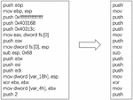
The gene obtained from the above steps is the complete assembly code. To make the subsequent operations such as gene cleaning and similarity calculation more efficient, this paper uses the opcode sequence to represent the gene, as shown in Figure 1.
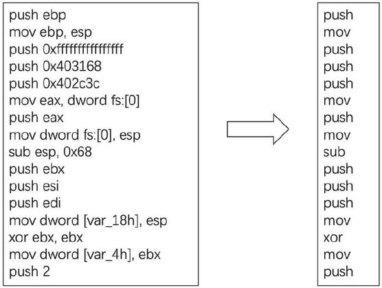
Figure 1 Software gene diagram.
3.2 Gene Clean
The extracted genes also have a large number of genes that are not related to the core function of the malicious code, so it is also necessary to remove a large amount of noise from the software genes to better obtain genes that can characterize a certain class of APT features. In this paper, the TF-IDF (term frequency-inverse document frequency) algorithm is used for the classification process. The main idea of the algorithm is that if a word appears in an article with a high TF frequency and rarely in other articles, the word or phrase is considered to have a good category differentiation ability and is suitable for classification.
In this system, the TF-IDF algorithm is used to select genes with high frequency in a certain family sample and low frequency in other family samples of the APT sample as the characteristic genes of that family. For gene x in a particular APT sample, the TF value is calculated as shown in Equation (1).
| (1) |
is the number of APT samples of that class containing gene x; A is the total number of APT samples of that class.
Calculate the IDF value as shown in Equation (2).
| (2) |
N is the total number of APT types and N(x) is the number of APT types containing gene x in a given family sample set.
The higher the TF-IDF value obtained by solving Equation (3).
| (3) |
The better the gene can characterize that class of APT traits. In this paper, the TF-IDF values of all genes of each sample were found and ranked. The top 400 genes were selected as the characteristic genes for that sample.
3.3 Gene Cluster
In APT sample analysis, functionally similar APT sample genes will to some extent also present morphologically similar sequences, and therefore highly similar genes can be considered as genes that are essentially functionally identical and can be grouped into one category. Based on this property of software genes, this system uses the Word2Vec algorithm to vectorize the gene sequences represented by the opcode, and in turn, uses the cosine distance to calculate the cosine similarity of the two vectors.
After obtaining the word vectors using Word2Vec, we chose to compare the similarity of two genes using the gene distance measure, followed by clustering all genes in the database using the UPGMA (Unweighted Pair Group Method with Arithmetic Mean) clustering algorithm. The UPGMA algorithm constructs a rooted tree (dendrogram) that reflects the presence of a pairwise similarity matrix (or dissimilarity matrix) in the structure. At each step, the two closest clusters are combined into a higher-level cluster. Any two clusters of size A and B are the average of the distances d(x,y) of all objects x in A and all objects y in B. Thus, the distance between any two clusters is defined in Equation (4).
| (4) |
For this system, genes with similar functions often have similar sequences, so closely related genes are grouped together to reduce dimensionality. The clustering algorithm relies on defining distance, accomplished here using the Smith-Waterman algorithm, a method for local sequence alignment that identifies the most similar subsequence between two sequences. This algorithm is beneficial for gene sequences, where only specific portions may be similar. It’s highly accurate and accommodates insertions or deletions common in gene sequences, though it’s computationally intensive, especially for long sequences. In our system, pre-processed genes are normalized into shorter sequences, mitigating computational costs for clustering. The main design idea is as follows.
Given two opcode representations of the gene sequences , and , where and are both opcodes, the highest score of the subsequence consisting of the first i elements of A and the subsequence consisting of the first j elements of B is recorded using a matrix starting from the starting elements of the two sequences, and the formula is given in Equation (5).
| (5) |
, . is the weight of the score deducted for mismatches of subsequences of length k. is the score value added when and in the sequence are matched successfully, and when the value is set to 1, is exactly equal to the length of the longest common subsequence of sequences A and B. The distance between sequence A and sequence B is defined in Equation (6).
| (6) |
Based on the gene distance measure, this paper adopts an optimized UPGMA clustering algorithm to cluster similar genes and then map them into a sample vector to achieve dimensionality reduction, while clustering makes the correlation of each dimension lower, which meets the requirements of machine learning for sample vectors. By iteratively executing the UPGMA algorithm to cluster the highly correlated genes, the dimensionality of sample vectors is gradually reduced and more suitable to be processed by the classical machine learning algorithms. In this paper, the number of clusters is set to 256, resulting in 256 clusters. For all genes in a sample, check whether a gene in one of the clusters exists, and if so, dispose of the corresponding vector position by 1, otherwise set it to 0, thus constructing a sample vector of length 256. This provides the input for subsequent machine-learning algorithms.
3.4 Detection
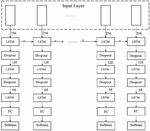
After the sample vectors are constructed, a multi-layered neural network architecture is employed for classification. Initially, a one-dimensional convolution-based neural network is used to process the input vectors. The one-dimensional convolutional layers are adept at capturing local dependencies and patterns within the sample vectors.
Following the convolutional layers, the architecture integrates a three-layer LSTM module to effectively model the sequential dependencies inherent in the APT sample data. A schematic diagram of the complete neural network structure, including the convolutional layers and the three-layer LSTM module, is illustrated in Figure 2.
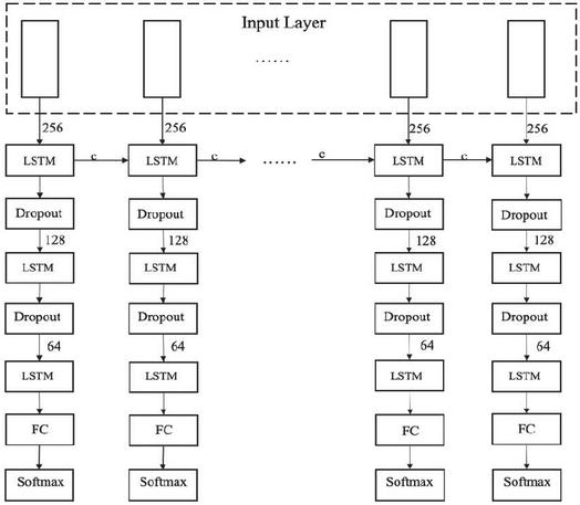
Figure 2 Neural network architecture diagram.
The first LSTM layer has 256 units and processes the initial feature representation derived from the convolutional layers. It captures the initial temporal relationships within the data. The output of the first LSTM layer is then fed into the second LSTM layer, which consists of 128 units. This layer further refines the temporal features and abstracts more complex patterns from the lower-level representations. Finally, the third LSTM layer with 64 units receives the output from the second layer and continues the process of temporal feature extraction. This hierarchical structure allows the network to capture temporal dependencies at different scales and levels of abstraction.
The output of the third LSTM layer is then directed towards a fully connected layer, which serves as the classifier. The fully connected layer transforms the high-level features learned by the LSTMs into a vector of length 2, representing the probabilities that a given sample is an APT or non-APT. This output is used to implement the APT detector.
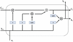
The LSTM-based APT detector contains a series of basic LSTM units forming the memory storage layer that stores the summary of the behavior of the processed APT samples. Figure 3 shows the architecture of LSTM unit.
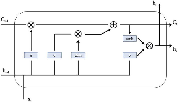
Figure 3 LSTM unit.
In each LSTM unit, the hidden output vector is passed from the LSTM cells to the fully connected (FC) layer and optimized using the Softmax function. The following recursive Equation (7) describe how these LSTM cells work.
| (7) |
Where is the sigmoid function, is element-wise product, is input vector, are linear transformation matrices, are the bias vectors, are the gating vectors, is the cell memory state vector, is the state output vector.
Each LSTM cell information memory updating, forgetting, and outputting its state is determined by the gating vectors . Then cell state and output are changed according to Equation (7), and whether the cell state is reset or restored is determined according to the state of the forgotten gate vector . The other two gating vectors, and , operate similarly to adjust the input and output.
3.5 Homology Determination
Malicious samples originating from the same APT group tend to have partially similar behavior or functions and genes can express behavior indirectly, so the number of genes shared by samples belonging to the same team tends to be larger. This paper employs the K-nearest Neighbor (KNN) algorithm for APT homology determination. It classifies samples based on the majority class of the k most similar samples in the feature space. The algorithm depends solely on the nearest sample’s category for classification. Similarly, if most of the k nearest neighbor samples belong to a category, the sample is classified accordingly.
KNN’s performance depends on K and distance definition. Small K values are sensitive to noise, while large K values may include distant samples, potentially biasing predictions. Uneven sample distribution can lead to significant errors. This paper measures proximity using shared gene count, considering samples closer if they share more genes, aligning with gene association mapping principles.
4 Evaluation
4.1 Environment and Dataset
The experimental environment for system testing in this paper is shown in Table 2 below.
Table 2 System test experiment environment
| Hardware/Software | Config | Detail |
| Hardware | CPU | Inter(R) Core(TM) i5-8300H |
| Memory | 16GB | |
| OS | Window 10, Ubuntu16.04 | |
| Software | Programming Languages | Python3.7, React |
| Development environment | Visual Studio Code |
The dataset of APT malicious samples used in the experiments is shown in Table 3 below. Special needs to be pointed out is that the dataset central to our study stands out for its direct use of original executable files from APT samples, offering a high-fidelity reflection of real-world scenarios. These raw samples were processed through our system to create a detection and classification framework that mirrors the challenges encountered in actual cybersecurity environments, where APT samples often lack labels and are scarce. By deliberately choosing a dataset that embodies these constraints, our model is rigorously tested and validated under conditions that cybersecurity systems face, enhancing its practical relevance and robustness.
| Config | Detail | Test Dataset | |
| APT 1 | 405 | 40 | |
| APT 10 | 244 | 24 | |
| APT 19 | 32 | 3 | |
| APT 21 | 106 | 10 | |
| APT 28 | 214 | 21 | |
| APT | APT 29 | 281 | 28 |
| APT 30 | 164 | 16 | |
| DarkHotel | 273 | 27 | |
| Energetic Bear | 132 | 13 | |
| Equation Group | 395 | 39 | |
| Gorgon Group | 961 | 96 | |
| Winnti | 387 | 38 | |
| Common Malware | 957 | 320 |
The dataset is from the APT Malware Dataset [23]. We use 3594 samples from 12 APT groups to build the APT gene database and map APT gene associations and use these APT samples and 957 common malicious samples for training the detection model. The system was tested using 355 samples from 12 APT groups and 320 common malicious samples. The trained APT detection model was first used to make predictions and test the performance of the model. Finally, the samples detected as APT are added to the genetic profile, and the changes in the genetic profile are demonstrated.
4.2 Detection Performance
Based on the neural network classifier detection model implemented in the previous section, this section uses the dataset shown in Table 3 for model training. The training set consists of 3876 samples, including 3239 APT samples and 637 non-APT samples, and the test set consists of 675 samples, including 355 APT samples and 320 non-APT samples. The test metrics include Accuracy, Precision, and Recall, which are calculated by Equations (8).
| (8) |
Where TP is the number of positive samples predicted as a positive class by the detection module; TN is the number of negative samples predicted as a negative class by the detection module; FP is the number of negative samples predicted as a positive class by the detection module; and FN is the number of positive samples predicted as a negative class by the detection module.
Firstly, a fully connected neural network-based classifier was constructed for experiments in this paper. The training environment and the deep learning framework used are shown in Table 4.
Table 4 Detection model test environment
| Environment | Detail |
| Test environment | Anaconda3-5.3.1, Python3.7 |
| framework | Pytorch1.11 |
The training parameters for the proposed detection model (the LSTM model) and the other contrast neural network detection models are shown in Table 5, using the Adam optimizer and setting the initial learning rate to 10-4, with the loss function using Cross Entropy Loss. There is a little difference between the input training data among these detection models, in which the input training data processed by DNN1, DNN2, 2D-CNN, VGG, and ResNet are the grayscale image features generated from the input malware samples, while the 1D-CNN and LSTM use the API features of samples.
Table 5 The Training parameters of different detection models
| DNN1 | 1D CNN | LSTM | 2D CNN | ||||
| Models | [18] | DNN2 [18] | [15, 16] | (Our Model) | [14, 17] | VGG | ResNet |
| Dense | 1024,1 | 1024,512,256,1 | 1024,1 | 1 | 1024,1 | 4096 | 2048 |
| Dropout | 0.01 | 0.01,0.01,0.01,0.01 | 0.5 | 0.1 | 0.5 | 0.5 | – |
| Activation | ReLU | ReLU, ReLU, ReLU | ReLU | – | ReLU | ReLU | ReLU |
| Batch size | 64 | 64 | 64 | 32 | 64 | 64 | 64 |
| Epochs | 200 | 200 | 200 | 200 | 200 | 200 | 200 |
| Pool size | – | – | 2 | – | 2 | 2 | 2 |
| Kernel size | – | – | 3 | – | 3 | 3 | 3 |
| Number of Filters | – | – | 64 | – | 64 | 64 | 64 |
The comparison results on performance metrics (etc. accuracy, precision, and recall rate) among the different detection models are listed in Table 6. The proposed detection model of the LSTM network has achieved the best scores on both accuracy, precision, and recall rate. The scale of the model architecture of the LSTM network is also more concise than the other neural network detection models.
Table 6 The comparison of performance metric results of different detection models
| DNN1 | 1D CNN | LSTM | 2D CNN | ||||
| Models | [18] | DNN2 [18] | [15, 16] | (Our Model) | [14, 17] | VGG | ResNet |
| Accuracy | 0.73 | 0.77 | 0.92 | 0.95 | 0.87 | 0.86 | 0.94 |
| Precision | 0.75 | 0.79 | 0.91 | 0.94 | 0.84 | 0.91 | 0.92 |
| Recall | 0.74 | 0.81 | 0.93 | 0.95 | 0.85 | 0.89 | 0.91 |
The comparison results of model training accuracy and loss among the different detection models are shown in Figure 4. With the increasing epochs of model training, the average accuracy/loss of the proposed LSTM detection model is higher/lower than the other detection models within the range of 25 to 200 epochs. The results show the best evaluation performance of the proposed LSTM-based detection model on APT samples identification and source classification, by which we can easily recognize the samples from the known APT groups or the common malware.
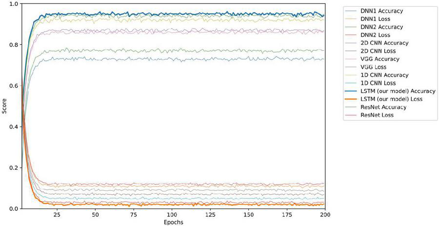
Figure 4 The accuracy and loss comparison among different detection models.
4.3 Homology Determination Evaluation
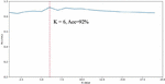
Based on the homology determination model implemented in the previous section, the system tested the homology determination on a gene pool formed by 3239 APT samples using the 335 APT samples in Table 3. The core parameter of the KNN algorithm is the value of K. The system tested the effect of the value of K on the accuracy of homology determination, and its relationship with the accuracy is shown in Figure 5.
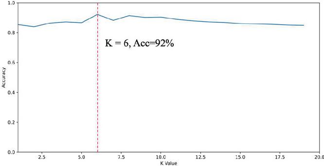
Figure 5 The impact of K value on classification results.
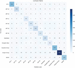
The false positive rate (FPR) and false negative rate (FNR) are calculated based on the confusion matrix generated from the classification results. The confusion matrix, as depicted in the appended Figure 6, elucidates the distribution of true positives, false positives, false negatives, and true negatives for each APT category. The FPR is determined by dividing the number of false positive occurrences by the sum of the false positives and true negatives, thereby offering insight into the frequency at which non-homologous samples are erroneously classified as homologous. Conversely, the FNR is obtained by dividing the number of false negative instances by the sum of false negatives and true positives, providing an understanding of the system’s tendency to misclassify homologous samples as non-homologous.

Figure 6 The confusion matrix.
Upon examination, it was observed that the FPR was notably higher for APT-19. This can be attributed to the inherent limitations of the KNN algorithm, where the classification decision is based on the majority voting among the nearest neighbors. APT-19, having a smaller representation in the dataset, is more susceptible to being overshadowed by other categories with larger sample sizes. Consequently, the FPR for APT-19 reflects the system’s challenge in robustly classifying sparsely represented categories.
This comprehensive evaluation framework, inclusive of FPR and FNR metrics alongside accuracy, allows for a more nuanced understanding of the system’s capabilities and limitations, thus facilitating informed operational decision-making when deploying the system in real-world scenarios.
4.4 APT Gene Association Map
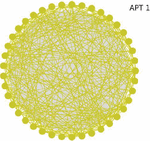
According to the method described in the previous section, the gene association map within each APT group was mapped in this paper. Figure 7 shows the association map within the APT-1 organization, which can visually show that there is obvious gene sharing between malicious codes originating from the same APT group, reflecting that the samples borrow more from each other and contain many similar behaviors and functions.
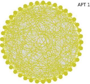
Figure 7 Gene association map of APT-1.
Based on the gene association mapping within the APT group, we plot the gene association mapping between APT groups. For any two different APT groups, if the number of shared genes present is greater than a set threshold, a line is used to label between the two APT groups, and the thickness of the line reflects the number of samples with shared genes. The complete gene association map is shown in Figure 8. It can be seen that most of the groups were associated with each other, but the association was weak.
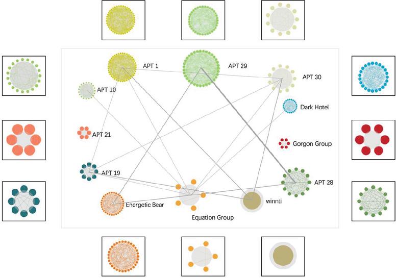
Figure 8 Gene association map among the APT groups.
There were strong genetic associations between APT-28, APT-29, and Energetic Bear groups, with APT-28 and APT-29 sharing the strongest degree of genes. It reached 4.2 in the evaluation index of this paper. Understanding correlations among APT groups benefits users in several ways:
(1) Enhancing Defensive Strategies: By comprehending APT attackers’ behavioral tendencies and TTPs, users can strengthen their defenses. For example, if certain APT groups prefer specific malware or attack methods, users can proactively implement countermeasures.
(2) Rapid Response: Knowing the relationships among APT groups helps users swiftly identify and respond to combined attacks. If two groups have collaborated before, unusual activity in one may indicate an impending attack, prompting a quicker response.
(3) Strategic Decision Making: Insights into APT group interconnections assist users in making informed strategic decisions. For instance, if users are frequently targeted by certain APT groups, they may allocate more resources to defend against these threats.
5 Conclusions
APT attacks pose significant threats to enterprise and national network security. This paper addresses the limitations of traditional feature code matching technology, which struggles to identify new malware. It proposes a scheme for malware identification through genetic mapping, drawing inspiration from biological genetics to correlate malware and conduct homology analysis. The paper designs a homology determination system for APT samples. Initially, the system extracts APT sample genes by merging basic blocks of software code, applies the TF-IDF algorithm to screen for characteristic genes, and constructs gene features using the word2vec algorithm. A three-layer LSTM-based classifier detects APT samples, while the KNN algorithm determines APT sample homology. Gene mapping facilitates the rapid and accurate identification of APT attack characteristics, enhancing detection efficiency. Experimental results demonstrate continuous enrichment of the APT gene map during detection, enabling comprehensive APT association presentations and sample detection capabilities. Users can interact with the gene map to understand APT group associations and detect APT attacks by uploading samples. This system resolves the challenge of accurately identifying APT attack code presence and traceability in malware.
References
[1] Chen Ruidong, Zhang Xiaosong, Niu Weina, Lan Haoyue. “A Research on Architecture of APT Attack Detection and Countering Technology.” Journal of University of Electronic Science and Technology of China, 2019, 48(6): 870–879.
[2] Xiong C L, Zhu T T, Dong W H, et al. “Conan: A Practical Real-Time APT Detection System With High Accuracy and Efficiency.” IEEE Transactions on Dependable and Secure Computing, 2022, 19(1): 551–565.
[3] Panahnejad M, Mirabi M. “APT-Dt-KC: advanced persistent threat detection based on kill-chain model,” Journal of Supercomputing, 2022, 78(6): 8644–8677.
[4] QiAnXin Threat Intelligence Center. “Global Advanced Persistent Threat Report.” https://ti.qianxin.com/uploads/2022/03/31/4217b248a07f1f1c42b4bba4168efb4e.pdf.
[5] Cen L, Gates C S, Si L, et al. “A Probabilistic Discriminative Model for Malware Detection with Decompiled Source Code.” IEEE Transactions on Dependable & Secure Computing, 2015, 12(4): 400–412.
[6] Kwon B J, Mondal J, Jang J, et al. “The Dropper Effect: Insights into Malware Distribution with Downloader Graph Analytics,” the 22nd ACM SIGSAC Conference on Computer and Communications Security, ACM, 2015:1118–1129.
[7] Garbervetsky D, Zoppi E, Livshits B. “Toward full elasticity in distributed static analysis: the case of callgraph analysis,” 11th Joint Meeting of European Software Engineering Conference (ESEC)/ACM SIGSOFT Symposium on the Foundations of Software Engineering (FSE), ACM, 2015: 442–453.
[8] Rosenberg I, Sicard G, David E O. “DeepAPT: Nation-State APT Attribution Using End-to-End Deep Neural Networks,” 26th International Conference on Artificial Neural Networks, Springer, 2017: 91–99.
[9] Pascanu R, Stokes J W, Sanossian H, et al. “Malware Classification with Recurrent Networks,” 2015 IEEE International Conference on Acoustics, Speech and Signal Processing, IEEE, 2015: 1916–1920.
[10] Miller B, Kantchelian A, Tschantz M C, et al. “Reviewer Integration and Performance Measurement for Malware Detection,” 13th International Conference on Detection of Intrusions and Malware, and Vulnerability Assessment, 2016: 122–141.
[11] Huang Y Z, Qiao M, Liu F D, et al. “Binary code traceability of multigranularity information fusion from the perspective of software genes,” Computers & Security, 2022, 114.
[12] Zhao B L, Zhang S, Liu F D, et al. “Malware homology identification based on a gene perspective,” Frontiers of Information Technology & Electronic Engineering, 2019, 20(6): 801–815.
[13] Zhao X L, Zhang Y M, L X H, et al. “Research on malicious code homology analysis method based on texture fingerprint clustering,” 17th IEEE International Conference On Trust, Security And Privacy In Computing And Communications/12th IEEE International Conference On Big Data Science And Engineering, IEEE, 2018: 1914–1921.
[14] Sun G, Qian Q. Deep learning and visualization for identifying malware families. IEEE Transactions on Dependable and Secure Computing, 2018.
[15] Zhang Z, Qi P, Wang W. Dynamic malware analysis with feature engineering and feature learning. In: Proceedings of the AAAI conference on artificial intelligence, vol. 34, (01), 2020, p. 1210–7.
[16] Li C, Zheng J. API call-based malware classification using recurrent neural networks. Journal of Cyber Security and Mobility, 2021;617–40.
[17] Chaganti R, Ravi V, Pham TD. Deep learning based cross architecture internet of things malware detection and classification. Computers & Security, 2022;102779.
[18] Chaganti R, Ravi V, Pham T D. A multi-view feature fusion approach for effective malware classification using Deep Learning. Journal of information security and applications, 2023.
[19] Do Xuan, C., Dao, M.H. A novel approach for APT attack detection based on combined deep learning model. Neural Comput & Applic 33, 13251–13264 (2021). https://doi.org/10.1007/s00521-021-05952-5.
Biographies

Rui-chao Xu received the bachelor’s degree in electrical engineering and automation from North China Electric Power University in 2001. He is currently working as a senior engineer at the State Grid Liaoning Electric Power Supply Co., Ltd. His research areas include power system automation and network security.

Yue-bin Di received the bachelor’s degree in agricultural electrification and automation from Shenyang Agricultural University in 2001. He is currently working as a senior engineer at the State Grid Liaoning Electric Power Supply Co., Ltd. His research areas include power system automation and network security.

Zeng Shou received the bachelor’s degree in automation from University of Science and Technology Beijing in 1997. He is currently working as a senior engineer at the State Grid Liaoning Electric Power Supply Co., Ltd. His research areas include power system automation and network security.

Xiao Ma received the bachelor’s degree in information science and engineering from Northeastern University in 1998. He is currently working as a senior engineer at the NARI Group Corporation (State Grid Electronic Power Research Institute) and Beijing Kedong Electric Power Control System Co., Ltd. His research areas include industrial automation and network security.

He-qiu Chai received the bachelor’s degree in software engineering from Northeastern University in 2021, and studying for the master degree at Northeastern University. His research areas include software security and network security.

Long Yin received the master’s degree in software engineering from JiLin University in 2016, and studying for the Ph.D. degree at Northeastern University. His research areas include cryptography and network security.
Journal of Cyber Security and Mobility, Vol. 13_4, 751–774.
doi: 10.13052/jcsm2245-1439.1348
© 2024 River Publishers