Network Security Behavior Anomaly Detection Based on Improved Empirical Mode Decomposition

Xiaowu Li

School of Mechanical Engineering, University of Science and Technology Beijing, Beijing, 100083, China
E-mail: xiaowu_li1214@126.com

Received 14 December 2023; Accepted 13 April 2024

Abstract

The current network behavior features have high latitude and complex components, making it difficult for existing temporal analysis techniques to perform temporal analysis and anomaly detection. To this end, a multi-scale decomposition module based on improved empirical mode decomposition is proposed and combined with generalized likelihood theory to construct a time series analysis model. The dataset decomposition experiment showed that the improved empirical mode decomposition proposed in the study had certain advantages in the decomposition performance of the three datasets, but it was difficult to judge the difference between normal time series and time series data with anomalies only from the perspective of periodicity. The validation experiment of anomaly detection in the time series analysis model showed that applying data augmentation effectively improved the detection performance of the time series analysis model. Compared with other methods, the proposed time series analysis model had an increase in true class rate of 1.23%–5.13%, and a decrease in false positive class rate of 19.05%–4.00%. Feature selection effectively improved the anomaly detection ability of temporal analysis technology, and the true class rate of temporal analysis technology based on feature selection increased by 1.27%–8.96%. Ranking temporal data according to feature importance for anomaly detection effectively increased the effectiveness of anomaly detection. The True Positive Rate (TPR) value of anomaly detection for temporal data with the highest feature importance was as high as 0.93. The results indicate that improved empirical mode decomposition can effectively meet the temporal data decomposition of high latitude network behavior characteristics, and the proposed temporal analysis model has better applicability and efficiency in temporal data anomaly detection. The temporal analysis model based on improved empirical mode has a more accurate recognition rate and lower false alarm rate in dealing with temporal data anomaly detection in different network environments, and has certain practical value in the field of network security behavior anomaly detection.

Keywords: Empirical mode decomposition, generalized likelihood ratio, time series data analysis, data augmentation, channel integration, TPR.

1 Introduction

With the development of network technology, the internet has become an essential part of people’s daily lives, and people are becoming increasingly dependent on the internet. The Internet not only affects people’s work, learning, and social interaction, but also has been widely used in fields such as medicine, industry, and military [1]. However, while the internet brings convenience, it is also accompanied by the leakage of personal privacy, virtual property, etc. The increase in the size of network users has led to an increasingly complex network topology. Therefore, effective implementation of network security protection has become an urgent problem to be solved [2, 3]. The application and development of digital computers have driven the application value of time series data. Using network behavior characteristics as time series data to detect network conditions has become an important means of network security behavior anomaly detection [4, 5]. However, the characteristics of network behavior are generally characterized by high latitude and complex components, and current research methods are difficult to fully meet the needs of effective temporal analysis [6]. In this context, research proposes to improve empirical mode decomposition (EMD) based on optimizing the complete set of adaptive noise, and combines Improved Complete Ensemble Empirical Mode Decomposition with Adaptive Noise (ICEEMDAN) with Generalized Likelihood Ratio Test (GLRT) to design a time series analysis model for multi-scale decomposition and multi-channel analysis. The time series analysis model, which is decomposed and detected through signal processing theory, will be used for network time series data detection, in order to achieve the analysis and anomaly detection of network behavior characteristic data in different network environments, thereby providing guarantees for the normal operation of network security and providing new ideas for the development of the field of network behavior analysis.

The overall structure of the study consists of four parts: The first part summarizes the relevant research achievements and shortcomings of time series analysis models and empirical mode decomposition at home and abroad. In the second part, a time series analysis model based on improved empirical mode decomposition was studied and designed. The third part conducted experiments and analysis on the proposed ICEEMDAN and time series analysis model. The fourth part summarizes the experimental results and points out future research directions.

2 Related Works

With the rapid development of internet technology, various aspects of human life, work, and social interaction are closely related to the internet. Efficient network security protection has gradually risen to become an important topic amongst researchers around the world. Zhao et al. proposed a generative adversarial network based on three change encoders to enhance the security and stability of system maintenance, resulting in a system log anomaly detection model with a detection rate increase of 27.8% compared to other models [7]. Sun et al. proposed an intrusion detection model based on attention mechanism to address the lack of security mechanisms in controller Local Area Networks (LANs) in vehicle network protocols, thereby achieving effective detection of controller LANs in different vehicles without the need for communication matrices [8]. Deng et al. designed a detection model that combines structural learning methods with graph neural networks to detect and explain deviations and anomalies between sensors, accurately capturing the correlation between sensors and allowing users to infer the cause of detected anomalies [9]. Jain et al. studied integrated technologies based on distributed machine learning to improve the current network security detection mechanism, and obtained a network attack detection model with a detection rate of up to 93% [10]. Hosseinzadeh et al. proposed a method for anomaly detection in network security by applying Support Vector Machine (SVM) to intrusion detection and security attacks, thereby achieving an effective combination of machine learning, artificial intelligence technology, and vector machine classifiers in network security detection [11].

Fourier transform and other time-frequency decomposition technologies have driven the development of data analysis, and the importance of signal decomposition technology has gradually increased. Studying it has become a new trend in the current computer field [12]. Mousavi proposed the introduction of adaptive noise technology on the basis of fully integrated empirical mode decomposition to solve the problem of signal nonlinearity and stability in bridge expansion and complex structures, thereby achieving effective bridge damage detection only when determining the location and severity of damage classification [13]. In order to improve the automatic detection effect of epileptic seizures, Li et al. designed an epileptic seizure detection method that combines empirical mode decomposition of long-term scalp computer images and common spatial patterns. This improved the detection sensitivity by 97.34% on the basis of segmentation and effectively improved the recognition and participation of EEG channels in epileptic seizures [14]. Krishnan et al. proposed a nonlinear signal quantization method based on randomness measure to improve the recognition of human psychological states in human-machine interface models, resulting in a classifier with an accuracy rate of up to 93.3% for recognizing human speech emotions [15]. Dwivedi et al. proposed a method that combines empirical mode decomposition based on stationary wavelet transform with integrated empirical mode decomposition to solve the problem of interpreting the original electrocardiogram signal of power signal infection. This approach achieved better signal-to-noise ratio enhancement while removing noise [16]. Long et al. proposed a method that combined empirical mode decomposition and wavelet thresholding to solve the problems of low recognition accuracy, low positioning accuracy, and weak detection effect on distant objects in unmanned target detection systems. This effectively removed seismic signal noise and preserved the target effective signal [17].

Overall, the current research on anomaly detection in network security behavior mainly focuses on the detection and protection of network devices, and there is relatively little research on the analysis and detection of network behavior feature data. The research on information decomposition technology mainly focuses on medical, military and other fields, and the research on empirical mode decomposition in network security detection is relatively shallow. Therefore, the study proposes the use of adaptive noise complete set technology to improve empirical mode decomposition, and combines its multi-scale decomposition module with GLRT to construct a time series analysis model. At the same time, the research innovatively integrates modal components into multiple channels after multi-scale module decomposition, and ranks temporal data according to importance features for anomaly detection. The research aims to improve the anomaly detection ability of temporal analysis technology in network operation by constructing multi-scale decomposition and multi-channel analysis models, providing theoretical support for network security, and promoting the practical application value of information decomposition technology in anomaly detection of network security behavior.

3 Time Series Analysis Model Construction Based on Improved Empirical Mode Decomposition

By analyzing temporal data and understanding its potential changes, information mining and anomaly detection can be ultimately achieved. Therefore, this study proposes to construct a temporal analysis model based on improved empirical mode and apply it to anomaly detection of network behavior features. The study of analyzing the temporal data characteristics of network features to determine the current network situation is of great significance for maintaining the normal operation of network security and reducing abnormal losses.

3.1 Multi-Scale Decomposition Module Construction Based on Improved Empirical Mode Decomposition

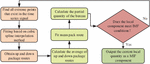
In order to decompose the network behavior characteristics into channels of different time scales, research proposes to use signal decomposition to reasonably separate the variation patterns of their aliasing. Signal decomposition refers to the decomposition of data signals based on the time scale of signal sequences, and empirical mode decomposition (EEM) is the core of this decomposition method [18]. The process of EEM decomposing temporal data signals is shown in Figure 1.

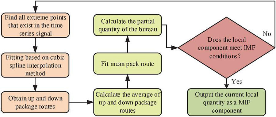
Figure 1 EEM decomposition process.

From Figure 1, it can be seen that first, all the extreme points of the time series signal are found, and then fitted using the cubic spline interpolation method to obtain the upper and lower envelopes. Based on the mean of the upper and lower envelopes, the fitted mean envelope is obtained. Secondly, the local components are obtained by subtracting the mean envelope from the original signal. Whether the local quantity meets the Intrinsic Mode Functions (IMF) is determined, and if it does not, the signal again is input until the condition is met to end the iteration. If the conditions are met, the current local quantity is treated as an IMF component and removed from the original signal to obtain the residual term. Decomposition is started again using the residual term as the input signal until the conditions are met. If the residual terms generated by decomposition do not meet the predetermined assumptions, EMD decomposition stops. Therefore, the final temporal signal expression is shown in formula (1).

$$s_t=\sum _{i=1}^n{\mathit{imf}}_{it}+r_t$$

(1)

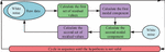
In formula (1), $s_t$ represents the timing data signal. ${\mathit{imf}}_{it}$ represents an IMF component. $r_t$ represents a residual term. However, EMD may experience modal aliasing when faced with noise signals and indirect signals. Therefore, research proposes to improve EMD using an optimized adaptive noise complete set to obtain an improved ICEEMDAN. The improved ICEEMDAN decomposition process is shown in Figure 2.

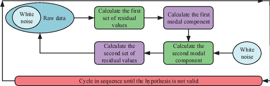
Figure 2 ICEEMDAN decomposition process.

As shown in Figure 2, a set of white noise is first added to the original data, a new sequence is obtained based on the given time series data, and the first set of residual values and modal components are calculated. Next, white noise will be continued to be added and local mean decomposition will be used to calculate the second set of residual values and the second modal component. The obtained multiple sets of IMF components will be averaged to obtain the final IMF component. The calculation formula for the new sequence is shown in formula (2).

$$x_i=x+{\beta }_{i-1}E(w_i)$$

(2)

In formula (2), $x_i$ represents the calculated new sequence of numbers. $E$ represents an IMF component of a signal’s EMD decomposition. $w_i$ represents Gaussian white noise. The calculation formula for the first set of residual values is shown in formula (3).

$$R_{i=1}=(N(x_i))$$

(3)

In formula (4), $N$ represents the local mean of the input signal. The formula for calculating the first set of modal components is shown in formula (4).

$$d_{i=1}=x-R_{i=1}$$

(4)

In formula (4), $d_{i=1}$ represents the first set of modal component formulas. The residual values of the second and subsequent groups are shown in formula (5).

$$R_{i+1}=R_i+{\beta }_{i}E(w_i)$$

(5)

The formula for calculating the second and subsequent modal components is shown in formula (6).

$$d_{i+1}=R_i-(N(R_i+{\beta }_{i}E(w_i)))$$

(6)

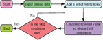
On this basis, the study utilizes ICEEMDAN to construct a multi-scale decomposition module, which is used to analyze the preprocessed feature data with the highest importance. The specific steps are shown in Figure 3.

Figure 3 The process of ICEEMDAN multi-scale decomposition module.

As shown in Figure 3, a series of data with the highest importance is input into ICEEMDAN for scale decomposition. By adding the decomposed white noise, the IMF component is calculated. The IMF component has different time scales and frequency characteristics, and the low-frequency IMF component can affect the analysis results. Therefore, the study also introduces channel integration technology to process the ICEEMDAN decomposition results. The processing method is shown in Figure 4.

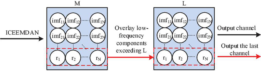
Figure 4 Channel integration process.

From Figure 4, it can be seen that when the decomposed IMF component exceeds the pre-set number of channels, channel integration will stack the residual term and the low-frequency IMF component exceeding the number of channels as the last channel, reducing the impact of low-frequency IMF components on model performance and ensuring the integrity of temporal data information.

3.2 Multiscale Decomposition and Time Series Analysis Model Based on Improved Empirical Mode Decomposition

In order to improve the detection ability of time series analysis, a multi-scale decomposition and generalized Likelihood Ratio Test (MDGLRT) is constructed by combining GLRT with improved ICEEMDAN. GLRT is a multi-channel temporal detection technology that obtains multi-channel temporal data sets by deploying multiple sensors [19, 20]. The expression formula for the temporal data set is shown in formula (7).

$$X=\left[\begin{array}{cccc}\hfill x_1^1\hfill & \hfill x_1^2\hfill & \hfill \mathrm{\cdots }\hfill & \hfill x_1^n\hfill \\ \hfill x_2^1\hfill & \hfill x_2^2\hfill & \hfill \mathrm{\cdots }\hfill & \hfill x_2^n\hfill \\ \hfill \mathrm{⋮}\hfill & \hfill \mathrm{⋮}\hfill & \hfill \mathrm{\ddots }\hfill & \hfill \mathrm{⋮}\hfill \\ \hfill x_L^1\hfill & \hfill x_L^2\hfill & \hfill \mathrm{\cdots }\hfill & \hfill x_L^n\hfill \end{array}\right]=\left[\begin{array}{c}\hfill x_1^T\hfill \\ \hfill x_2^T\hfill \\ \hfill \mathrm{⋮}\hfill \\ \hfill x_L^T\hfill \end{array}\right]$$

(7)

In formula (7), $T$ represents the set of times. $L$ represents a multidimensional dataset collected at a time node. Since the rows and columns of the time series data contain the time series data and the spatial information contained by different sensors respectively, the formula obtained by quantizing the matrix columns is shown in formula (8) [21, 22].

$$z=vec(X^T)$$

(8)

In formula (8), $z$ represents the matrix obtained by quantifying the columns of the temporal data matrix $X$. According to the calculation, the covariance matrix of matrix Z is obtained, as shown in formula (9).

$$Y=E[z{z}^H]=\left[\begin{array}{cccc}\hfill Y_{11}\hfill & \hfill Y_{21}^H\hfill & \hfill \mathrm{\cdots }\hfill & \hfill Y_{L1}^H\hfill \\ \hfill Y_{21}\hfill & \hfill Y_{22}\hfill & \hfill \mathrm{\cdots }\hfill & \hfill Y_{21}^H\hfill \\ \hfill \mathrm{⋮}\hfill & \hfill \mathrm{⋮}\hfill & \hfill \mathrm{\ddots }\hfill & \hfill \mathrm{⋮}\hfill \\ \hfill Y_{L1}\hfill & \hfill Y_{L2}\hfill & \hfill \mathrm{\cdots }\hfill & \hfill Y_{LL}\hfill \end{array}\right]$$

(9)

In formula (9), $H$ represents conjugate transposition. The matrix $Y$ collects the spatiotemporal information of the data within the matrix $X$, but GLRT has assumptions in the process of detecting temporal signals. Therefore, the assumption is defined as the null hypothesis and the alternative hypothesis binary hypothesis. The expression formula for both is shown in formula (10).

$$\{\begin{array}{c}\phi :z\sim ℂ\mathbb{N}(0_{LN},Y_{\phi }),Y_{\phi }\in {\mathrm{\Re }}_{\phi }\hfill \\ \varphi :z\sim ℂ\mathbb{N}(0_{LN},Y_{\varphi }),Y_{\varphi }\in {\mathrm{\Re }}_{\varphi }\hfill \end{array}$$

(10)

In formula (10), $\phi$ represents the null hypothesis. $\varphi$ represents alternative hypothesis. $Y_{\phi }$ and $Y_{\varphi }$ represent two different covariance matrices. ${\mathrm{\Re }}_{\phi }$ represents the space where the covariance matrix does not contain relevant spatiotemporal feature structures. ${\mathrm{\Re }}_{\varphi }$ represents the space where the partitioned diagonal covariance matrix is located. The physical significance of the binary hypothesis is that under the null hypothesis, the covariance matrix is a zero matrix when two time series data are unequal, indicating that there is no spatiotemporal correlation between the two time series data, thus indicating that $\varphi$ does not have this property [23–25]. Signal detection requires multiple samples to obtain a better probability representation. Therefore, based on the vectorized temporal signal matrix, the joint probability density of the samples is obtained, as shown in formula (11).

$$p(z[1],\mathrm{\dots },z[M];Y)=\frac{1}{{\pi }^{LNM}det{(Y)}^M}\exp \{-Mtr(Y^{-1}\widehat{Y}\}$$

(11)

In formula (11), $p(z[1],\mathrm{\dots },z[M];Y)$ represents the joint probability density of the vectorized matrix. $M$ represents the total number of independent copies of the timing signal. $\widehat{Y}$ represents the sample covariance matrix, which is calculated as shown in formula (12).

$$\widehat{Y}=\frac{1}{M}\sum _{m=0}^{M-1}Z[m]z^H[m]$$

(12)

In formula (12), $m$ represents the number of individual independent copies. According to the above calculation formula, the expression of the generalized likelihood ratio of time series samples under the binary assumption is shown in formula (13).

$$\gamma =det{({\widehat{Y}}_0^{-1}{\widehat{Y}}_1)}^M\exp \{-Mtr[({\widehat{Y}}_0^{-1}-{\widehat{Y}}_1^{-1}]\widehat{Y}\}$$

(13)

In formula (13), $\gamma$ represents the generalized likelihood ratio. ${\widehat{Y}}_0$ and ${\widehat{Y}}_1$ represent the maximum likelihood estimates of the sample under different assumptions, respectively. Due to the fact that time-domain GLRT is not affected by linear transformation, its expression after linear transformation is shown in formula (14).

$${\gamma }^{\frac{1}{M}}=det({\widehat{Y}}_0^{-1}{\widehat{Y}}_1)=det(\widehat{C})$$

(14)

In formula (14), $\widehat{C}$ represents a coherent matrix, and its specific calculation expression formula is shown in formula (15).

$$\widehat{C}=\frac{{\widehat{D}}^{-\frac{1}{2}}}{\widehat{Y}{\widehat{D}}^{-\frac{1}{2}}}$$

(15)

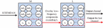
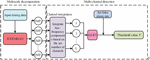
In formula (15), $\widehat{D}$ represents a diagonal matrix. According to the above formula, the overall structure of the MDGLRT proposed in the study is shown in Figure 5.

Figure 5 MDGLRT model structure.

From Figure 5, it can be seen that MDGLRT is mainly composed of two parts: a multi-scale decomposition module and a multi-channel timing analysis module. Firstly, the preprocessed network behavior features are used as temporal signals for multi-scale decomposition. Secondly, the obtained IMF components are integrated into channels. Finally, the network features are classified and detected for any anomalies.

4 Time Series Analysis Model Validation Based on Improved Empirical Mode Decomposition

The MDGLRT proposed in the study used multi-channel detection of temporal data, fully utilizing the correlation between the spatiotemporal features present in temporal data. By mapping network temporal data to channels at different time scales, the changes in temporal data at each scale were analyzed to extract anomalous temporal data. Therefore, by validating models on multiple different datasets and comparing their performance with some current temporal analysis techniques, it was beneficial to promote the innovation of temporal analysis techniques and improve their practical value in network security behavior detection.

4.1 Verification of Multi-Scale Decomposition Module Based on Improved Empirical Mode Decomposition

In order to verify the decomposition performance of the multi-scale decomposition module based on the ICEEMDAN proposed in the study, the CICIDS-2017 dataset, UNSW-NB15 dataset, and MAWILab dataset were selected for performance verification. Firstly, the three datasets were preprocessed separately, and the training and testing sets were sorted based on the importance of the preprocessed data features for ICEEMDAN decomposition. The feature importance ranking of the three datasets after preprocessing is shown in Table 1.

Table 1 Ranking of feature importance after preprocessing of three datasets

CICIDS-2017 dtasets	UNSW-NB15	MAWILab
Importance	Feature	Importance	Feature	Importance	Feature
Ranking	Name	Ranking	Name	Ranking	Name
1	IP-OUTBPS	1	SYN-FROM-PEERS	1	RST-TO-PEERS
2	IP-INBPS	2	OTHERIP-FROM-PEERS	2	UDP-FLOWS
3	TCP-OUTBPS	3	TCP-FLOWS	3	UDP-FROM-PEERS
4	TCP-INBPS	4	RST-FROM-PEERS	4	DNS-FROM-PEERS
5	RST-FROM-PEERS	5	UDP-OUTBPS	5	SYN-TO-PORT-PEERS
6	SYN-TO-PEERS	6	TCP-FROM-PEERS	6	TCP-FROM-PEERS
7	UDP-TO-PEERS	7	AVGLEN-IN-TCPFLOW	7	IP-INBPS
8	PKTS-PER-TCPFLOW	8	TCP-TO-PEERS	8	TCP-TO-PEERS
9	TCP-FROM-PEERS	9	OTHERIP-FROM-PEERS	9	OTHERIP-TO-PEERS
10	RST-TO-PEERS	10	AVGLEN-OUT-UDPFLOW	10	RST-FROM-PEERS

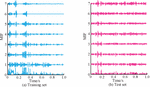
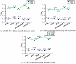
Based on the ranking results of importance, the top ten important features were selected as the experimental dataset to verify the effectiveness of the feature selection algorithm. Continuous normal data in the dataset was selected as the original dataset, and the data subset of the most important feature was decomposed into ICEEMDAN. The decomposition results of the training and testing sets of the CICIDS-2017 dataset are shown in Figure 6.

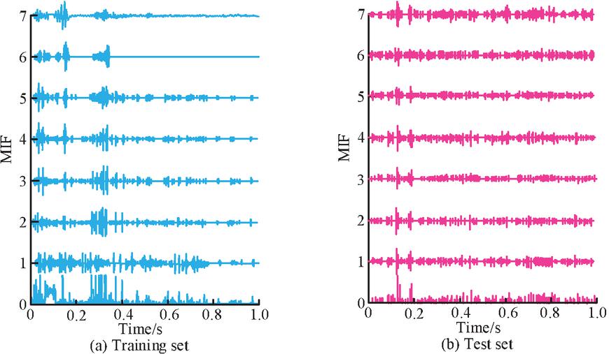
Figure 6 Decomposition results of training and testing sets for the CICIDS-2017 dataset.

From Figure 6, it can be seen that ICEEMDAN multiscale decomposition decomposed normal time series data and time series data containing anomalies onto multiple channels. The comparison between the training set and the test set showed that the larger the IMF component, the more significant the fluctuation of its decomposition curve. This indicated that the ICEEMDAN proposed in the study had good decomposition performance for temporal data. The decomposition results of the training and testing sets of the UNSW-NB15 dataset are shown in Figure 7.

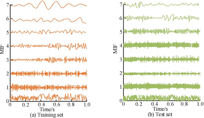
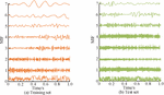
Figure 7 Decomposition results of training and testing sets for the UNSW-NB15 dataset.

From Figure 7, it can be seen that the IMF components of the training and testing sets obtained from the UNSW-NB15 dataset after ICEEMDAN decomposition in different cycles were determined based on the IMF components at the format component scale. The channel fluctuations under different IMF components in the test set were significantly higher than those in the training set, which may be due to the fact that the test set had more data than the training set and may contain abnormal temporal data. The decomposition results of the training and testing sets of the MAWILab dataset are shown in Figure 8.

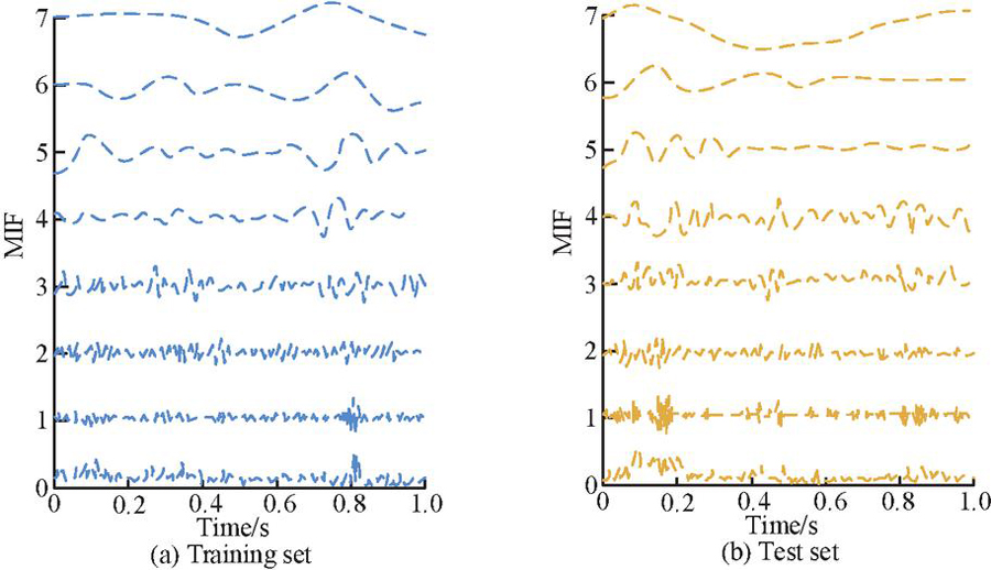
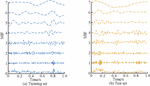
Figure 8 Decomposition results of training and testing sets for the MAWILab dataset.

From Figure 8, it can be seen that the decomposition results of the MAWILab dataset were different from the multi amplitude fluctuations of the first two datasets, and the channel fluctuations were more stable after the IMF component was greater than 2. Overall, IMF components at different time scales had different periods, but it was difficult to determine the difference between normal time series and time series data with anomalies based solely on the period. Therefore, it was necessary to extract the intrinsic correlation of IMF components through multi-channel time series analysis technology. Therefore, the study further determined the channel based on the IMF components at each time scale and integrated the channels, and enhanced the data of the integrated channel data (DA+MDGLRT). Finally, by enhancing the dataset, the normal data GLRT values of the three datasets were calculated, and the temporal data under each time window was detected.

4.2 Verification of Anomaly Detection in Time Series Analysis Model Based on Improved Empirical Mode Decomposition

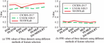
In order to validate the anomaly detection performance of the temporal decomposition model proposed in the study, based on the decomposition results of ICEEMDAN on the training and testing sets of three datasets, the detection performance of the model on temporal data was evaluated using two statistical indicators: false positive rate (FPR) and TPR [26, 27]. Meanwhile, SVM, K-NearestNeighbor algorithm (KNN), and Multilayer Perceptron (MLP), which are the current commonly used temporal analysis techniques, are introduced to compare the detection performance with the proposed method of the study [28–30]. The anomaly detection results of the three datasets are shown in Figure 9.

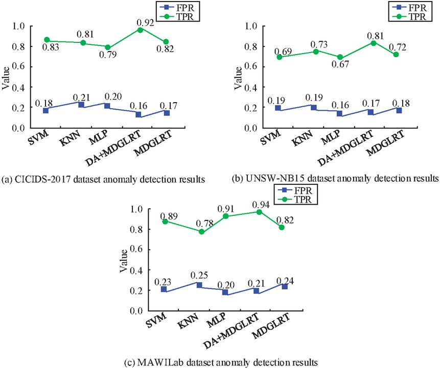
Figure 9 Comparison of anomaly detection results of different methods for three datasets.

From Figure 9(a), it can be seen that the TPR value of DA+MDGLRT obtained after data augmentation in the dataset CICIDS-2017 was the highest among all methods, and the FPR value was the lowest among all methods. This indicated that data augmentation effectively improved the anomaly detection ability of the time series analysis model. The lower the FRP value, the lower the false alarm rate of the detection method. The higher the TPR value, the more effective the detection method was for anomaly detection. The TPR value of MDGLRT was reduced by 1.20% compared to SVM, but its FPR value was lower than SVM, indicating that MDGLRT had certain advantages in false probability performance. In the UNSW-NB15 dataset in Figure 9(b), the TPR value of DA+MDGLRT was the highest among all methods, while the detection rate of MDGLRT was better than SVM and MLP. In the MAWILab dataset in Figure 9(c), MDGLRT with data augmentation still showed efficient detection performance, while MDGLRT without data augmentation had significantly lower detection and false positive rates than KNN. Overall, the MDGLRT proposed in the study had certain detection accuracy in detecting abnormal results, and its false probability was lower compared to other methods, making the detection results relatively more effective. On this basis, the study introduced feature selection subsets into three methods: SVM, KNN, and MLP to compare anomaly detection results. The specific results are shown in Figure 10.

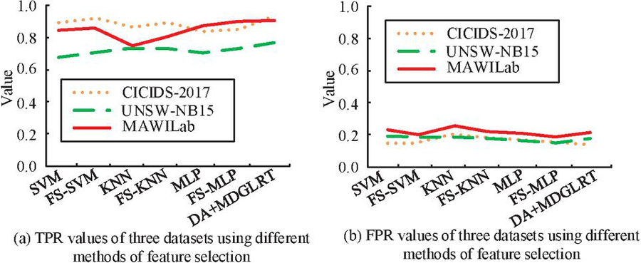
Figure 10 Introduction of different methods of feature selection for anomaly detection results in three datasets.

From Figure 10, it can be seen that the TPR values of SVM, KNN, and MLP methods all increased to varying degrees after feature selection for detection, while the FPR values relatively decreased. This indicated that feature selection before anomaly detection in temporal data effectively improved the detection performance of temporal analysis techniques. However, overall, the detection rate and false alarm rate of DA+MDGLRT with data augmentation were still superior to the three methods after feature selection. In addition, the study further applied the importance ranking features to anomaly detection, and the anomaly detection results of the three datasets are shown in Table 2.

From Table 2, it can be seen that sorting the features of temporal data by importance before anomaly detection resulted in a detection effect that was directly proportional to the importance of the features. Among them, the detection rate of the first important feature in the CICIDS-2017 dataset increased by 184.38% compared to the tenth, the detection rate of the first important feature in the UNSW-NB15 dataset increased by 60.78% compared to the tenth, and the detection rate of the first important feature in the MAWLab dataset increased by 97.87% compared to the tenth. This indicated that the higher the importance of data features, the higher their TPR value, and the better the anomaly detection results. It can be seen that sorting temporal data features according to their importance had a certain auxiliary effect on improving the detection ability of temporal analysis technology.

Table 2 TPR value under feature importance ranking

CICIDS-2017 datasets		UNSW-NB15		MAWILab
Feature Name	TPR	Feature Name	TPR	Feature Name	TPR
IP-OUTBPS	0.91	SYN-FROM-PEERS	0.82	RST-TO-PEERS	0.93
IP-INBPS	0.84	OTHERIP-FROM-PEERS	0.79	UDP-FLOWS	0.89
TCP-OUTBPS	0.82	TCP-FLOWS	0.76	UDP-FROM-PEERS	0.87
TCP-INBPS	0.71	RST-FROM-PEERS	0.73	DNS-FROM-PEERS	0.79
RST-FROM-PEERS	0.63	UDP-OUTBPS	0.69	SYN-TO-PORT-PEERS	0.74
SYN-TO-PEERS	0.58	TCP-FROM-PEERS	0.64	TCP-FROM-PEERS	0.68
UDP-TO-PEERS	0.53	AVGLEN-IN-TCPFLOW	0.59	IP-INBPS	0.62
PKTS-PER-TCPFLOW	0.49	TCP-TO-PEERS	0.57	TCP-TO-PEERS	0.58
TCP-FROM-PEERS	0.44	OTHERIP-FROM-PEERS	0.56	OTHERIP-TO-PEERS	0.42
RST-TO-PEERS	0.32	AVGLEN-OUT-UDPFLOW	0.51	RST-FROM-PEERS	0.47

5 Result and Discussion

The period of the channel is closely related to the distance and the storage capacity of the information, and the IMF component of smaller period is used as the input of the data enhancement module. Multi-channel decomposition of the time-series data in the dataset to obtain the IMF component is helpful to accurately obtain the threshold value for detecting anomalies, so as to effectively detect the information in the channel. The study performed multi-channel decomposition on three datasets, and the results showed that the larger the IMF component is, the more obvious the fluctuation of its decomposition curve is. This was also confirmed by Chen et al. who performed a time series analysis of periodic fluctuation using EMD and gray-wave prediction model [31].

However, the detection of anomalous time series is not effectively achieved based on the IMF component alone. Therefore, the study further utilizes the proposed multiscale decomposition module with the time-series analysis model for performance testing in three datasets and compares it with the current popular methods. The results show that the proposed method of the study is more superior in terms of FPR and TPR. The reason for this result may be due to the fact that the kernel function of SVM and the setting of the relevant parameters affect its anomaly detection performance. Sharmila et al. conducted a time series study using three algorithms, SVM, KNN, and Gradient Boosting Decision Tree, and found that the unimproved SVM and KNN algorithms were slower to analyze the temporal analysis, which led to poorer anomaly detection results [32]. This is consistent with the results obtained from the study.

The use of improved empirical modal decomposition of time-series signals and the construction of the MDGLRT model in combination with GLRT show some superiority in performance validation, though. However, it has different performance effects in different datasets. In the dataset with less normal time series data, the proposed preprocessing method can significantly improve the detection results of the algorithm, but its performance is average without data enhancement, which may be due to some limitations of the proposed method itself. However, overall, the ICEEMDAN-based MDGLRT model is still significantly better than the current popular methods.

6 Conclusion

In order to conduct temporal analysis of high latitude and complex network behavior characteristics, a multi-scale decomposition module is proposed based on improved empirical mode decomposition, and combined with GLRT to construct an MDGLRT model. The validation of the multi-scale decomposition module shows that ICEEMDAN has certain advantages in decomposing the three datasets, but it is difficult to judge the difference between normal time series and time series data with anomalies only from the cycle. It is necessary to extract the intrinsic correlation of its IMF component through multi-channel time series analysis technology. The validation experiment of anomaly detection in the time series analysis model showed that applying data augmentation effectively improved the detection performance of MDGLRT. The TPR values of MDGLRT in the three datasets increased by 1.23% $-$5.13% compared to other methods, and the anomaly detection effect was the best in the CICIDS-2017 dataset. Feature selection effectively enhanced the anomaly detection ability of time series analysis technology and reduced its false alarm rate and false probability. Ranking temporal data according to feature importance for anomaly detection effectively increased the effectiveness of anomaly detection. The TPR value of anomaly detection for the most important feature in the three datasets was as high as 0.93. The above results indicate that the multi-scale decomposition module and temporal analysis model proposed in the study have superior applicability and efficiency, and have a more accurate recognition rate and lower false alarm rate for anomaly detection of temporal data in different network environments. However, there are still certain shortcomings in the research, as there are differences in detection and false alarm rates among different datasets, and the information with different features in temporal data has not been extracted. In the future, research will further explore the MDGLRT model’s anomaly detection of temporal data in multi column features.

References

[1] Y. Fang, B. Luo, T. Zhao, D. He, B. Jiang, Q. Liu, ‘ST-SIGMA: Spatio-temporal semantics and interaction graph aggregation for multi-agent perception and trajectory forecasting’; CAAI Trans Intell Technol, vol. 7, pp. 744–757, 2022.

[2] W. Kim, Y. Park, J. Shin, M. Jo, ‘Consumer preference structure of online privacy concerns in an IoT environment’, International Journal of Market Research, vol. 64, pp. 630–651, 2022.

[3] O. Omiunu, I. A. Aniyie, ‘Sub-national involvement in nigeria’s foreign relations law: an appraisal of the heterodoxy between theory and practice’, African Journal of International and Comparative Law, vol. 30, pp. 252–269, 2022.

[4] Y. Wang, L. Du, ‘Change-detection-assisted multiple testing for spatiotemporal data’, J Stat Plan Inference, vol. 227, pp. 57–74, 2023.

[5] L. Wang, J. Zhao, Z. Xu, F. Zhao, C. Song, C. Yang, ‘Integrated energy system optimal operation using data-driven district heating network model’, Energy Build, vol. 291, pp. 1–16, 2023.

[6] A. M. Tomczyk, M. W. Ewertowski, ‘Landscape degradation and development as a result of touristic activity in the fragile, high-mountain environment of Vinicunca (Rainbow Mountain), Andes, Peru’, Land Degradation & Development, vol. 34, pp. 3953–3972, 2023.

[7] Z. Zhao, W. Niu, X. Zhang, R. Zhang, Z. Yu, C. Huang, ‘Trine: syslog anomaly detection with three transformer encoders in one generative adversarial network’, Applied Intelligence: The International Journal of Artificial Intelligence, Neural Networks, and Complex Problem-Solving Technologies, vol. 52, pp. 8810–8819, 2022.

[8] H. Sun, M. Chen, J. Weng, Z. Liu, G. Geng, ‘Anomaly detection for in-vehicle network using CNN-LSTM with attention mechanism’, IEEE Trans Veh Technol, vol. 70, pp. 10880–10893, 2021.

[9] A. Deng, B. Hooi, ‘Graph neural network-based anomaly detection in multivariate time series’, Proc AAAI Conf Artif Intell, vol. 35, pp. 4027–4053, 2021.

[10] M. Jain, G. Kaur, ‘Distributed anomaly detection using concept drift detection based hybrid ensemble techniques in streamed network data’, Cluster Computing, vol. 24, pp. 2099–2114, 2021.

[11] M. Hosseinzadeh, A. M. Rahmani, B. Vo, M. Bidaki, M. Masdari, M. Zangakani, ‘Improving security using SVM-based anomaly detection: issues and challenges’, Soft Computing, vol. 25, pp. 3195–3223, 2021.

[12] C. Deng, Y. Huang, N. Hasan, Y. Bao, ‘Multi-step-ahead stock price index forecasting using long short-term memory model with multivariate empirical mode decomposition’, Information Sciences, vol. 607, pp. 297–321, 2022.

[13] A. A. Mousavi, C. Zhang, S. F. Masri, G. Gholipour, ‘Structural damage detection method based on the complete ensemble empirical mode decomposition with adaptive noise: A model steel truss bridge case study’, Structural Health Monitoring, vol. 21, pp. 887–912, 2021.

[14] C. Li, W. Zhou, G. Liu, Y. Zhang, M. Geng, Z. Liu, W. Shang, ‘Seizure onset detection using empirical mode decomposition and common spatial pattern’, IEEE Trans Neural Syst Rehabil Eng, vol. 29, pp. 458–467, 2021.

[15] P. T. Krishnan, A. N. Joseph Raj, V. Rajangam, ‘Emotion classification from speech signal based on empirical mode decomposition and non-linear features: Speech emotion recognition’, Complex & Intelligent Systems, vol. 7, pp. 1919–1934, 2021.

[16] A. K. Dwivedi, H. Ranjan, A. Menon, P. Periasamy, ‘Noise reduction in ECG signal using combined ensemble empirical mode decomposition method with stationary wavelet transform’, Circuits Syst Signal Process, vol. 40, pp. 827–844, 2021.

[17] L. Long, X. Wen, Y. Lin, ‘Denoising of seismic signals based on empirical mode decomposition-wavelet thresholding’, J Vib Control, vol. 27, pp. 311–322, 2021.

[18] M. Chai, Z. Gao, Y. Li, Z. Zhang, Q. Duan, R. Chen, ‘An approach for identifying corrosion damage from acoustic emission signals using ensemble empirical mode decomposition and linear discriminant analysis’, Measurement Science & Technology, vol. 33, pp. 1–19, 2022.

[19] R. E. Vieceli, D. A. Dodge, ‘Assessing the effectiveness of generalized likelihood ratio test detector schemes in seismic event detection and the avoidance of nontarget signals’, Bulletin of the Seismological Society of America, vol. 112, pp. 1384–1396, 2022.

[20] B. Zaman, ‘Efficient adaptive cusum control charts based on generalized likelihood ratio test to monitor process dispersion shift’, Qual Reliab Eng Int, vol. 37, pp. 3192–3220, 2021.

[21] Yu J, Li X, Guan X, Shen H. A remote sensing assessment index for urban ecological livability and its application. Geo-Spatial Information Science, 2024, 27(2): 289–310.

[22] Wang Y, Xu Y, Yang J, Wu M, Li X, Xie L, Chen Z. Fully-connected spatial-temporal graph for multivariate time-series data. In Proceedings of the AAAI Conference on Artificial Intelligence, 2024, 38(14): 15715–15724.

[23] Li L, Cheng J, Bannister J, Mai X. Geographically and temporally weighted co-location quotient: an analysis of spatiotemporal crime patterns in greater Manchester. International Journal of Geographical Information Science, 2022, 36(5): 918–942.

[24] Nephin J, Thompson P L, Anderson S C, Park A E, Rooper C N, Aulthouse B, Watson J. Integrating disparate survey data in species distribution models demonstrate the need for robust model evaluation. Canadian Journal of Fisheries and Aquatic Sciences, 2023, 80(12): 1869–1889.

[25] Torreblanca E, Real R, Camiñas J A, Macias D, García-Barcelona S, Báez J C. Spatial and temporal partitioning of the Western Mediterranean Sea by resident dolphin species. Mediterranean Marine Science, 2023, 24(1): 34–49.

[26] B. Zhang, Y. Gao, J. Wu, N. Wang, Q. Wang, J. Ren, ‘Approach to predict software vulnerability based on multiple-level n-gram feature extraction and heterogeneous ensemble learning’, International journal of software engineering and knowledge engineering, vol. 32, pp. 1559–1582, 2022.

[27] G. Jull, J. Treleaven, ‘Response rate and comparison of clinical features associated with positive or negative responses to a scapular positioning test in patients with neck pain and altered scapular alignment: a cross-sectional study’, BMJ Open, vol. 11, pp. 435–459, 2021.

[28] E. A. G. Venugopal, ‘A comparative analysis on hybrid svm for network intrusion detection system’, Turkish Journal of Computer and Mathematics Education, vol. 12, pp. 2674–2679, 2021.

[29] J. Qiu, X. Yan, W. Wang, W. Wei, K. Fang, Skeleton-based abnormal behavior detection using secure partitioned convolutional neural network model’, IEEE J Biomed Health Inform, vol. 26, pp. 5829–5840, 2021.

[30] Y. Labiod, A. Amara Korba, N. Ghoualmi, ‘Fog computing-based intrusion detection architecture to protect iot networks’, Wireless Personal Communications, vol. 125, pp. 231–259, 2022.

[31] Chen Y, Liu B, Wang T. Analysing and forecasting China containerized freight index with a hybrid decomposition–ensemble method based on EMD, grey wave and ARMA. Grey Systems: Theory and Application, 2021, 11(3): 358–371.

[32] Sharmila R B, Velaga N R, Kumar A. SVM-based hybrid approach for corridor-level travel-time estimation. IET Intelligent Transport Systems, 2019, 13(9): 1429–1439.

Biography

Xiaowu Li, Doctor of Engineering, Lecturer. Graduated from the Beijing University of Aeronautics and Astronautics in 2005. Worked in School of mechanical engineering, University of Science and Technology Beijing. His research interests include enterprise information system design; computer graphics and information security.

Journal of Cyber Security and Mobility, Vol. 13_5, 917–940.
doi: 10.13052/jcsm2245-1439.1355
© 2024 River Publishers

Abstract

1 Introduction

2 Related Works

3 Time Series Analysis Model Construction Based on Improved Empirical Mode Decomposition

3.1 Multi-Scale Decomposition Module Construction Based on Improved Empirical Mode Decomposition

3.2 Multiscale Decomposition and Time Series Analysis Model Based on Improved Empirical Mode Decomposition

4 Time Series Analysis Model Validation Based on Improved Empirical Mode Decomposition

4.1 Verification of Multi-Scale Decomposition Module Based on Improved Empirical Mode Decomposition

4.2 Verification of Anomaly Detection in Time Series Analysis Model Based on Improved Empirical Mode Decomposition

5 Result and Discussion

6 Conclusion

References

Biography