Study on the Application of Dynamic Continuous Trust Assessment Model Based on Clustering Mechanism in Network Security Optimization
Weidong Wu1,*, Zheng Tian2, Yizhen Sun2, Yongfa Li2 and Yu Cui3
1State Grid Hunan Electric Power Company Limited ChangSha, HuNan 410007, China
2Information and communication branch of State Grid Hunan Electric Power Company ChangSha, HuNan 410007, China
3State Grid Informationn & Telecommunication Group CO., LTD. 102211
E-mail: touran@139.com
*Corresponding Author
Received 18 September 2024; Accepted 09 December 2024
Abstract
Due to the rapid development of network technology and the increasing size of networks, the security of networks in today’s society is facing great challenges. The study of network security is based on the study of network security frameworks, connections, and models to improve network security so that the network becomes controllable, manageable, and survivable. In this paper, we propose a dynamic continuous trust assessment model based on the clustering mechanism and apply this model to the network security model optimization problem. The specific conclusions are as follows: (1) The problems in previous clustering algorithms are analyzed, and corresponding solutions are proposed for the problems. Then, the particle swarm algorithm is briefly introduced, the inertia weight coefficients in the particle swarm algorithm are improved, and the dormant mechanism of neighboring node groups is introduced. (2) A new algorithm for calculating direct trust value is proposed. (3) A method for evaluating the overall trust value level of the network is proposed. The method first selects the N nodes with the highest number of interactions and then evaluates the overall trust level of the network in which these N nodes are located by using the associative memory capability of the clustering algorithm. (4) The experimental analysis shows that the randomly generated rule set in the model of this paper tends to evolve to a stable state after 6080 rounds of operation, with a higher success rate, and at 180200 rounds of operation, the rule set evolves to a stable state again, with the success rate still improved; after 240 rounds of operation, the network environment is restored to the initial state, and although the roles of some of the nodes are changed, the model still evolves to a high level again. Level. The dynamic continuous trust evaluation model proposed in this paper can be effective in the network security optimization, but the practical application of the model should be done further research.
Keywords: Security in mobile networks, cyber-physical security, clustering algorithm, dynamic persistent trust.
Introductory
With the increasing size of the network, network attacks and destructive behaviors are increasing day by day, network security problems are becoming more and more prominent, and the network trust problem has also attracted much attention. In the past, passive network defense gradually changed to active defense, but the traditional network trust model can no longer meet current needs, and research on the network trust model has become increasingly urgent. In recent years, much domestic research has been done on the above problems. Liang Hua and other [1] proposed a node evaluation method based on the Internet of Things that the existing node evaluation method can not effectively deal with the malicious behavior of nodes so that they cannot resist the internal attacks of the network. However, the application of the improved method that cannot effectively deal with the malicious behavior of nodes is not elaborated. Li Huanhuan [2] elaborated and analyzed the advantages and disadvantages of the traditional network security model, and elaborated the architecture of the zero trust network security model. On this basis, taking the practice of the zero trust network security model on a network information security support technology platform as an example, and proposed the security application solution based on the zero trust architecture. Although the advantages and disadvantages of the traditional network security model are mentioned, it does not deeply analyze the comparative effect with the zero-trust model in specific scenarios, and lacks quantitative evaluation. Li Jinhua [3] proposed a trust evaluation model based on the entropy weight method. In the process of the fusion calculation of multi-dimensional decision attributes, the information entropy theory is used to establish the classification weight of each decision attribute, so as to avoid the problem that the subjective judgment method is not adaptable in the weight setting, and ensure the effectiveness and objectivity of the recommendation trust evaluation decision. Although the information entropy theory is mentioned, the lack of elaboration of its application mechanism in the trust assessment model makes it difficult for the reader to understand the theoretical support of the model. Liu and [4] proposed an active security model, starting from the analysis of security protection mechanism, based on the different perspectives of service providers and requesters, and the introduction of network risk assessment and trust assessment of user history interaction, to dynamically provide active protection ability for system resources to improve security. The trust assessment of the user history interaction behavior is mentioned, but the source, processing mode and analysis model of the behavioral data are not elaborated, which may reduce the reliability of the trust assessment. The above studies mainly focus on the construction of network security model, and there are few studies on the optimization of existing network models. In order to study the optimization of the existing network security model, this paper proposes a dynamic continuous trust assessment model based on the clustering mechanism and applies this model to the network security model optimization problem. It is of guiding significance to the existing network security optimization problem.
1 Cluster Algorithm for Sensor Networks in Wireless Networks
1.1 Classical Cluster Algorithm
Wireless networked sensor networks (WSNs) are typically deployed in harsh environments that are difficult for humans to approach, such as battlefields, forests, and specialized industrial and clinical areas. Therefore, WSNs need to have self-configuration capabilities and autonomous modes. Sensor nodes are typically equipped with batteries that cannot be recharged, and energy efficiency is a major consideration in order to extend the life cycle of the network, with data transmission being the main source of energy consumption. Moreover, as the size of the network of nodes increases, designing and operating such large-scale networks requires scalable architectures and management strategies. For large-scale networks, topology control balances the network load, increases network scalability, and extends the network life cycle. The clustering technique is an effective way to address energy efficiency, network scalability, and topology control, as shown in Figure 1. To achieve specific goals, task scheduling, data acquisition, and transmission power control [5–7] can also be used in clustered structures.
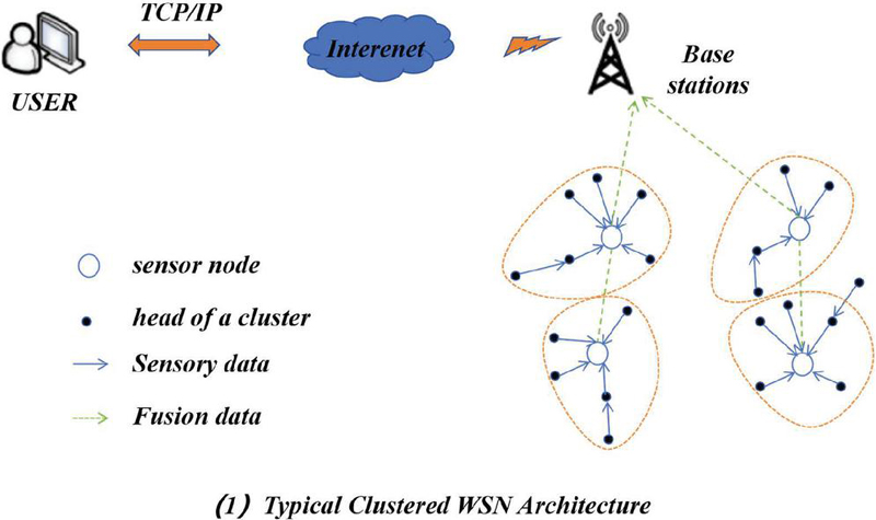
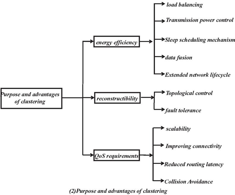
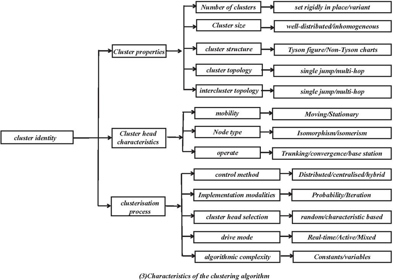
Figure 1 Cluster technology.
(1) LEACH algorithm LEACH is one of the most essential clustering algorithms. The fundamental thinking of LEACH is to rotate the cluster head amongst all the nodes to acquire load balancing. In LEACH, the execution time of the algorithm is measured in ’rounds, and every spherical is divided into two phases: cluster advent segment and stabilization phase [8, 9]. The algorithm creates clusters in the establishment phase, and in the stabilization phase, the cluster head transmits data directly to the base station. In the cluster establishment phase, each sensor node n selects a random number from 0 to 1. If this number is smaller than the threshold value , then this node becomes the cluster head and can be defined as
| (1) |
where p is the expected percentage of cluster heads among sensor nodes, r is the current round, and G is the set of nodes that have not become cluster heads in the last 1/p round. Figure 2(1) shows the topology of LEACH during the clustering process.
(2) HEED algorithm HEED is an iterative cluster-based algorithm that uses a combination of residual energy and communication overhead to select cluster heads. After the cluster head selection, the cluster heads in the network send data to the base station using a multi-hop transmission mechanism[10]. Cluster head selection consists of three main phases: the initialization phase, the repetition phase, and the final phase. In the initialization phase, each sensor node sets its probability of becoming a cluster head defined as follows:
| (2) |
Where is the optimisation percentage of cluster heads, usually set to 5%, which only affects the initial number of cluster heads and has no direct effect on the final number of cluster heads.
(3) BCDCP algorithm The iterative cluster splitting algorithm distributes the cluster heads uniformly in the network by maximising the distance between the cluster heads during each split. The topology of the BCDCP algorithm is shown in Figure 2(2).
(4) DWEHC algorithm This algorithm is an enhancement of HEED; however, it achieves greater desires than HEED, such as producing extra balanced cluster sizes and optimizing the intra-cluster topology through the use of the positional statistics of the nodes [11]. DWEHC creates a multilevel shape for intra-cluster conversation and additionally restricts the number of kids of a dad or mum node. In the cluster head selection process, the weights of each node are calculated as follows:
| (3) |
where R is the cluster range, and d is the distance from node s to neighboring node u.
Figure 2(3) shows its intra-cluster topology.
(5) PEGASIS algorithm This algorithm is an enchancment on HEED however achieves greater desires than HEED such as producing extra balanced cluster sizes and optimising the intra-cluster topology the use of the positional statistics of the nodes. DWEHC creates a multilevel shape for intra-cluster conversation and additionally restricts the quantity of kids of a dad or mum node. Figure 2(4) shows the data transmission mechanism of PEGASIS.
(6) EEUC algorithm This is a dispensed aggressive clustering algorithm in which cluster heads are chosen via nearby competition. Each node has a pre-specified aggressive range, i.e., the cluster size, a parameter that relies upon the distance between the node and the base station [12]. The closer to the base station, the smaller the cluster size, and the network topology is shown in Figure 2(5). It is calculated as follows:
| (4) |
(7) SEP algorithm This algorithm constructs clusters based on the energy heterogeneity of the nodes. There are two types of nodes in the network: some nodes with low initial energy are called ordinary nodes, and some other nodes with high initial energy are called advanced nodes[13-14]. The weighted probabilities are defined as follows for normal and advanced nodes, respectively:
| (5) | |
| (6) |
where is the optimized probability of a node being a cluster head, and m is the proportion of advanced nodes among all nodes.
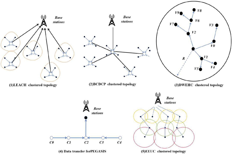
Figure 2 Classical clustering algorithm.
Here are seven classical clustering algorithms and their advantages and disadvantages:
1. LEACH algorithm
Advantages: simple and easy to understand, easy to implement; good effect on large-scale data sets, fast operation speed; can process high-dimensional data.
Disadvantages: cluster K; sensitive to initial value, results may be different; susceptible to outliers; only applicable to convex clusters.
2. HEED
Advantages: A dendrogram (dendrogram) can be obtained without assigning the cluster number in advance; it can provide clustering results at different levels for easy analysis.
Disadvantages: high computational complexity, especially when handling large data sets; sensitive to noise and outliers; once merged or split.
3. BCDCP
Advantages: It can find clusters of arbitrary shape and handle data of heterogeneous density; naturally identify noise points, do not need to specify the number of clusters.
Disadvantages: sensitive to parameter selection, especially the neighborhood size e.; Poor performance in high-dimensional data is prone to a “curse of dimensions”.
4. DWEHC
Advantages: Enough to deal with clusters with different covariances, suitable for data with different shapes, provides the probability that each point belongs to a certain cluster, and can deal with fuzzy classification.
Disadvantages: the need to preset the cluster number K; a more complex model, the high computational cost is sensitive to the initial value, may fall into the local optimum.
5. PEGASIS
Advantages: Without pre-specified cluster number, automatically detect cluster center; can handle clusters of arbitrary shape.
Disadvantages: high computational complexity, especially in high dimensional space; sensitive to bandwidth parameters, improper selection will affect the effect.
6. EEUC
Advantages: can capture the complex cluster structure, suitable for non-convex shape clusters; using the graph theory method, transform the data into the graph form, good results.
Disadvantages: high computational complexity, difficult to process large-scale data; requires preset cluster number K.
7. SEP
Advantages: It can form an adaptive cluster center; it can generate a better clustering effect, especially when the data amount is small.
Disadvantages: high computational cost, especially with large data volume; high sensitivity to input data (such as similarity matrix).
1.2 Improved Particle Swarm Based Cluster Algorithm (IPSO-CA)
1.2.1 Particle swarm algorithm
Suppose there is a particle in a dimensional space with a corresponding fitness function to determine whether the particle’s current position is optimal or not. The main parameter vectors in the algorithm are as follows:
The position of the ith particle and the velocity vector is:
| (7) | |
| (8) |
The fitness function of particle i is:
| (9) |
The optimal position vector that particle i passes through is:
| (10) |
The optimal position vector through which the whole population passes is:
| (11) |
Throughout the course of the iterative process, the position and velocity of particle I are updated by the equation:
| (12) | |
| (13) | |
| (14) | |
| (15) |
1.2.2 Improved particle swarm algorithm
In the standard particle swarm algorithm, the inertia weight coefficient w is a fixed value that cannot control the movement speed of the particles, and there is no way to control the accuracy of finding the optimal solution. There are many algorithms that improve the inertia weight coefficient so that w can be varied with the number of iterations, and the most popular one is the linear decreasing strategy [15–18]. The most used strategy is the linear decreasing strategy [19].
| (16) |
The specific improvement measures include:
Dynamic adjustment of the speed and position update formula
Adaptive weight: the inertial weight (w) is dynamically adjusted according to the number of iterations, which is large at the beginning and gradually decreases in the later stage to enhance the local search ability.
Variable speed update: the update formula to adjust the speed under specific conditions, introducing the time factor, so that the search speed decreases at convergence.
Introducing a hybrid strategy
Combined with other algorithms: combine PSO with other optimization algorithms such as genetic algorithms and ant colony algorithms to form a hybrid optimization strategy, and use the advantages of different algorithms to improve performance.
Local search mechanism: on the basis of the global search, the local search strategy is introduced to make the fine adjustment after the particle convergence to improve the accuracy of the solution.
Enhance the particle diversity
Diversity retention mechanism: Introduce diversity retention strategies when updating particle positions, for example, increasing the coverage of the search space by randomly disturbing or reset the position of certain particles.
Population differentiation: particles are divided into multiple subgroups, and search * * in different subgroups to enhance the global exploration ability.
Improved fitness assessment
Fuzzy fitness evaluation: fuzzy logic is introduced to evaluate fitness to reduce the uncertainty in fitness evaluation and improve the robustness of the algorithm.
Multi-objective optimization: For multi-objective problems, the Pareto frontier strategy is adopted to achieve the balance of multiple objectives through weight adjustment.
Introduce learning mechanism
History learning: introduce the best particle information in history, use the past successful search experience to guide the current search, and enhance the effectiveness of optimization.
Social learning: allows particles to influence the speed and position of other particles in the updating process, and improves the effect of group cooperation through social learning mechanism.
Introducing restrictions
Constraint processing mechanism: consider the constraints when updating the particle position to ensure that the particles are always in the feasible solution space. The penalty function or correction strategy can be used to handle the particles that do not meet the constraints.
Parameter-adaptive adjustment
Adaptive parameter adjustment: The algorithm parameters, such as the acceleration constants (c1 and c2), are dynamically adjusted according to the current search progress to accommodate the different search stages.
Termination criteria optimization
Intelligent termination criteria: introduce more complex termination criteria, for example, when the fitness change in multiple iteration periods is less than a certain threshold, avoiding unnecessary calculation.
1.2.3 Neighbourhood node groups
After the network initialization, the distance formula (17) obtains the distance between nodes, and preset a distance threshold. If the distance between nodes is less than the value, that is, the monitoring area of the two nodes is considered repeated, and the data information collected by the two nodes is the same. If both nodes are working, there will be unnecessary data redundancy [20, 21].
| (17) |
If both nodes are working at this point, then there will be unnecessary data redundancy. Each node in the set decides whether to participate in the current round or not based on the amount of energy; the node with more energy is active and performs the information collection and data forwarding operations, while the node with less energy is in a dormant state, and when a round is over it compares the energy and selects it again, and then starts the next round of work [22–24].
1.2.4 Optimal cluster head analysis
The optimal cluster head number analysis is a method used to determine the optimal number of cluster heads in a wireless sensor network. In a wireless sensor network, a cluster head is a special node responsible for collecting and processing data from surrounding nodes. To maintain network efficiency and energy efficiency, it is important to determine the appropriate number of cluster heads.
Energy equilibrium: A good cluster head selection strategy should be able to achieve the node energy equilibrium. This means that the chosen cluster heads should be scattered throughout the network, avoiding the premature depletion of energy at some nodes without local region coverage or the communication disruption.
Distance optimization: Cluster head selection should optimize network performance by minimizing the average distance from the cluster head to the node it belongs to. Shorter distances can reduce energy expenditure and improve the reliability and efficiency of data transmission.
Network coverage: the optimal number of clusters should ensure the coverage of the entire network. Ensure that each area of the network has a sufficient number of cluster heads, and the coverage is appropriate, ensure that all nodes in the network can be covered by the cluster heads, and achieve effective data transmission and processing.
Load equalization: The optimal cluster head number analysis criterion should also consider the load equalization. Choosing too many cluster heads may result in a high load on some cluster heads in the network and a low load in others. Therefore, selecting the appropriate number of cluster heads can achieve load balancing and improve the overall performance of the network.
Network life cycle: The optimal cluster head number analysis criterion should also consider the life cycle of the network. Choosing the appropriate number of cluster heads can extend the lifetime of the network, effectively utilize the energy resources of the nodes, and reduce the waste of energy.
Assume that the area size of the WSN is in which randomly deployed nodes. After the introduction of neighboring node groups, all the sensor nodes are divided into nodes n, which are not joined to any neighboring node group, wake-up nodes n, and dormant nodes n, and the number of cluster head nodes is, and on average, there is about one node in each cluster. The energy consumption of cluster head nodes in each round is given by Equation (18), and the energy consumption of normal nodes in each round is given by Equation (19):
| (18) | |
| (19) | |
| (20) |
The total energy consumption of the whole network per round is:
| (21) | ||
| (22) | ||
| (23) | ||
| (24) |
1.2.5 Analysis of simulation results
Figure 3(1) compares the networks of 4 one of a kind algorithms. It can be considered that the existence cycle of the LEACH algorithm and LEACH-C algorithm is around 800 rounds and a thousand rounds, respectively, and the lifestyles cycle of the PSO algorithm is around 1500 rounds, which improves the community lifetime with the aid of about 1 and 1/2 instances in contrast with LEACH and LEACH-C algorithm respectively, and the IPSO-CA algorithm proposed in this paper prolongs the community existence cycle to round 1900 rounds, which has greater apparent enhancement than the different algorithms. The IPSO-CA algorithm proposed in this paper extends the community lifespan to about 1900 rounds, which is more apparent than different algorithms. From the analysis of the above fact, it can be viewed that the IPSO-CA algorithm can certainly equalize the strength consumption of the nodes and lengthen the operation time of the network. Figure 3(2) compares the time of demise of specific numbers of nodes for the four algorithms. The IPSO-CA algorithm proposed in this paper has the first node dying time of around five hundred rounds, whilst the three different algorithms have node deaths of around 100, 200, and three hundred rounds, respectively. Compared to different algorithms, the IPSO-CA algorithm has a higher balance in the pre-running duration of the community.
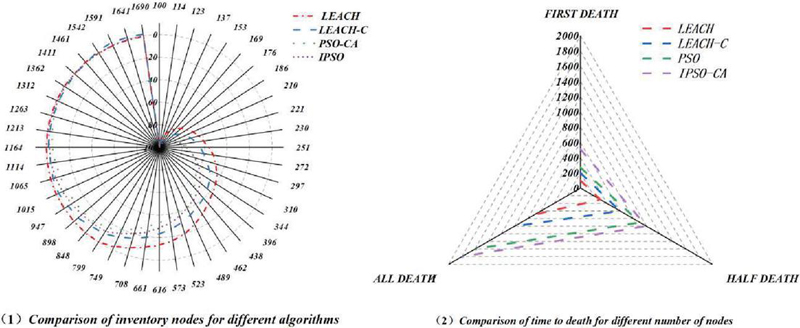
Figure 3 The life cycle of four different algorithmic networks.
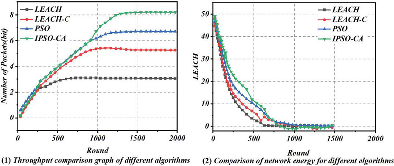
Figure 4 Network throughput and total residual energy of four different algorithms network.
Figure 4(1) compares the community throughput of the four algorithms. When the community is stable, the community throughput of the LEACH-C algorithm is about 5.3 104bit, the PSO algorithm is about 6.8 104bit, the IPSO-CA algorithm is about 8.2 104bit, and the use of the PSO algorithm and IPSO-CA algorithm can lead to a greater throughput of the network. The throughput of LEACH and LEACH-C algorithms stabilizes around five hundred rounds, whilst the throughput of the PSO algorithm and IPSO-CA algorithm stabilizes around five hundred rounds. The throughput of LEACH and LEACH-C algorithms stabilizes around five hundred rounds, whilst PSO and IPSO-CA algorithms stabilize around 800-1000 rounds. It can be considered that the IPSO-CA algorithm has higher performance. Figure 4(2) compares the whole residual community electricity of the four algorithms in every round. The complete community electricity of all 4 algorithms decreases steadily with the expansion of the wide variety of rounds; however, it is apparent that the curve of the IPSO-CA algorithm decreases extra slowly due to the fact some nodes of IPSO-CA algorithm live on for a longer time, which can be attributed to the reasonableness of the algorithm’s determination of the cluster head nodes and the sleep mechanism of the neighboring node groups, which can stability the electricity consumption of the nodes very well, and some of the nodes can no longer take part in the work to shop energy. Nodes can no longer take part in the work in order to keep greater energy and consequently prolong the use of community time.
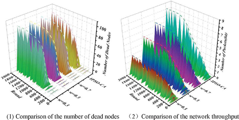
Figure 5 Number of dead nodes and throughput under different inertia weighting factors (w).
Figure 5(1) compares the number of dead nodes for different inertia weight factors (w). Analyzing the data in the figure, it can be seen that the IPSO-CA algorithm has the longest network lifecycle, and in the PSO algorithm, the network has the shortest lifecycle at the time. From the perspective of the network operation process, the node death time of the IPSO-CA algorithm is always the latest, which also proves that, compared with the PSO algorithm, the proposed IPSO-CA algorithm can better extend the network operation time and improve the network performance. Figure 5(2) compares the network throughput under different w. Analyzing the data, it can be seen that the IPSO-CA algorithm has the highest throughput after the network is stabilized, and in the HS algorithm, the network throughput is highest when w 0.7, and the network has the lowest throughput when w 0.3. It can be seen that the IPSO-CA algorithm performs better.
2 Dynamic Continuous Trust Assessment Model Based on Cluster Algorithm
2.1 Analysis of Trust Models
2.1.1 Trust model
In response to the fact that the PeerTrust model can only detect malicious nodes with malicious attack characteristics but cannot detect and punish nodes that collude in deception well, Chang Junsheng et al. proposed the DyTrust trust model. In the DyTrust trust model, the temporal characteristics of recommendation and experience are represented using time frames, and the trust of nodes is calculated by four parameters. By introducing a feedback control mechanism in the model, each parameter of node trust can be dynamically adjusted. These four parameters include long-term trust, near-term trust, feedback trustworthiness, and cumulative abuse of trust. “Feedback trust” refers to the degree of trust an individual or organization has in the reliability and effectiveness of others’ feedback during the interaction. This trust is usually affected by multiple factors, including the source of the feedback, the accuracy of the content, and the professionalism and experience of the feedbacks. In the DyTrust trust model, usually, the behavior between each node is normal and can complete the normal interaction process. Sometimes, the node with normal behavior will suddenly, after obtaining higher trustworthiness, turn to choose the zone to attack other nodes and become a malicious node with malicious aggressiveness, so the node’s trust value will be reduced, which leads to the concept of cumulative abuse of trust. In this model, it is stipulated that the sum of trust value reduction caused by malicious nodes attacking using higher trust values obtained from normal interaction behavior is called cumulative abuse of trust; nodes provide a large amount of feedback information, whether the information is trustworthy or not must be measured in a certain way, in order to solve this problem, the concept of feedback trustworthiness has been introduced into the DyTrust trust model. If the current time frame is n, then we can use the following algorithm to compute the trust of node u to node w:
ComputeTrust (u, w,n)
Input: w,n
0utput: Final trust value”
1. Feedback retieveFeedback(w,n)
2. FSer – Collection of Feedback Source Nodes in Feedback.
3. For i FSet do
Calculate Direct trust value: :
Feedback trust node i from Cache.:
Update Feedback trust :
end for
4. Calculate trust evaluation:
5. Update the factor a, , , and . of node w;
6. Calculate the final trust value on u to w.
2.1.2 Improvement of the trust model
In time frame n, the set of nodes excluding node i and interacting with node j is denoted as , denotes the direct trust of node i to j, is the confidence factor, and the more the number of interactions is, the larger its value is, and it is generally taken as h/H, with h being the number of interactions between i and j, and H being the minimum value of the number of interactions, and being its feedback trust. H is the minimum limit of interaction number and is its feedback trust. The formula for calculating the trust evaluation value of node i to node j is as follows:
| (25) |
is the satisfaction of interaction between node i and j, m is the number of node i, j interactions, and then the direct trust value is:
| (26) |
Since each node evaluates the public interaction nodes differently in each time frame, the feedback trustworthiness should then be updated in real-time, and for each time frame that passes, the evaluation value of the new node should be recorded. Therefore, we set , as the set of public interaction nodes of node i and node r in time frame n. If , then we can say that its evaluation is 0; at the same time, then the evaluation of node as well as feedback trust can then be expressed by Equations (27) and (28):
| (27) | ||
| (28) |
On the basis of the above trust evaluation value, the other three trust evaluation parameters of long-term trust, recent trust, and cumulative abusive trust can be calculated. Where the difference between the node’s trust and the actual empirical trust evaluation is taken as the abusive trust, and then the size of these three parameters above is compared, then the final trust evaluation result takes the smallest value of the three. Cumulative abusive trust is specifically used to penalize swinging nodes. Throughout the algorithm, the values of each parameter are updated all the time as the nodes interact with each other.
The recent trust value update is calculated
| (29) |
Update the calculation method for the cumulative abuse of trust values
| (30) |
Method of calculating the risk function
| (31) |
2.2 Application of Dynamic Continuous Trust Evaluation Model Based on Clustering Algorithm in Network Security
First, find the equilibrium point of the clustering algorithm network. The equilibrium point of the clustering algorithm neural network is the trust value of the ideal node of each level of a training sample given, and the ideal node trust value of each level we can obtain by finding the average of the trust value of each node corresponding to each different level of the sample. After the equilibrium point, you can use the associative memory function of the cluster algorithm network, the equilibrium point as a memory; once the input side of the network is classified as trust value input, the cluster algorithm network will go through a process of convergence from the initial input to the steady state, the network will use the function of associative memory to determine the weight coefficients in the network when gradually converging to a certain beginning of the equilibrium point, that is, the state of the network has reached stability, the network will use the function of associative memory to determine the weight coefficients in the network. That is, after the state of the network reaches stability, the network trust level is the classification level corresponding to the equilibrium point. The specific network trust evaluation algorithm is as follows:
Input: trust value of each node in the five random networks to be rated
Output: network trust level
1. obtain the trust value of 20 nodes in each of the five random networks through the A-Dytrust trust model;
2. find the equilibrium point through the ten samples of the ideal node trust level;
3. Design the ideal coding rules for node trust value levels;
4. Code the node trust value levels of each of the 5 random networks to be classified according to the coding rules of 3; design the coding rules of the ideal node trust level;
5. create the clustering algorithm;
6. set the initial state value of the clustering algorithm;
7. use the encoding of the trust values of the nodes of the five random networks to be rated as the input value of the neural network of the clustering algorithm;
8. Clustering Algorithm The neural network will converge to the equilibrium point through self-learning to obtain the network trust level. Network trust rating.
3 Simulation Analysis
In this paper, we refer to the simulation experimental environment setup proposed in the literature to simulate the interaction between nodes in a P2P network with Java programs. The difference is that in this paper, the size of the network is 5000 nodes, and each node has the six attributes defined in Section 4.2.1. Instead of responding correctly or maliciously deterministically, each node responds differently with a certain probability according to its different attributes. The model proposed in this paper requires a rule-set evolution process, and every 50 service requests submitted in the experiment is one round of the experiment, and the rule-set evolution is carried out once.
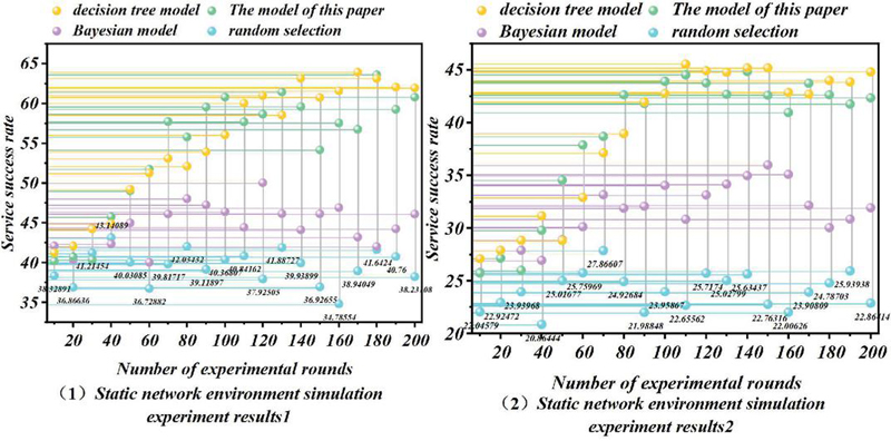
Figure 6 Experiments in a static network environment.
3.1 Static Network Environment Experiment
This experiment focuses on simulating the evaluation trust of each model when there is no major change in the network environment [25]. In this experiment, according to the experimental environment setup given in the previous section, each entity responds differently to service operations with certain probabilities based on its own state. These probability values are kept constant during the experiment, so the network environment is realized as a small change around a certain range in order to simulate a large-scale distributed computing environment. The experimental results are shown in Figure 6(1).
Experimental results show that in a static network environment, the success rate of the stochastic model fluctuates randomly up and down around 40%. The stochastic model reflects the basic situation of the dynamics of the network environment because each entity responds according to a certain probability in its own mode; the result of the response is bound to fluctuate up and down around a certain probability. As the number of participating nodes is large and dynamic, the probability of direct interaction experience between nodes is also small, so the Bayesian model has no significant improvement, and the success rate fluctuates around 46%. This also reflects that in the real network environment, it is not feasible to rely on the direct interaction experience to evaluate the entities because there is little direct interaction experience between the entities. In Experiment 2, we modify the parameters of the network environment so that the probability of providing the correct service operation in each entity’s behavioral pattern is reduced by 10%. To simulate the situation when the network environment performs poorly, the results of the experiment are shown in Figure 6(2).
3.2 Dynamic Network Environment Experiment
The setup of Experiment 3 focuses on the adaptability of each model to the dynamic changes in the network environment. The initial setting of Experiment 3 is the same as that of Experiment 1, but from 120 rounds of operation onwards, the setting is the same as that of Experiment 2. From 240 rounds of operation, the initial state is restored, but some of the nodes’ roles are changed, e.g., some of the original malicious nodes are changed to normal nodes, and some of the original normal nodes are changed to malicious nodes, etc. This is to simulate a large-scale change in the network environment. In this way, we simulate the situation when the network environment undergoes large-scale changes and examine the ability of each model to adapt to such large-scale changes. At the same time, we add the rule sets generated in Experiment 1 to the nodes as a simulation of the administrator’s manually specified fixed policies. That is, each node is fixed to use the rule set from the results of Experiment 1 as the policy to evaluate trust. In this way, we simulate the performance of trust models based on fixed policies or formulas and parameters under large-scale changes in the environment. The experimental results are shown in Figure 7.
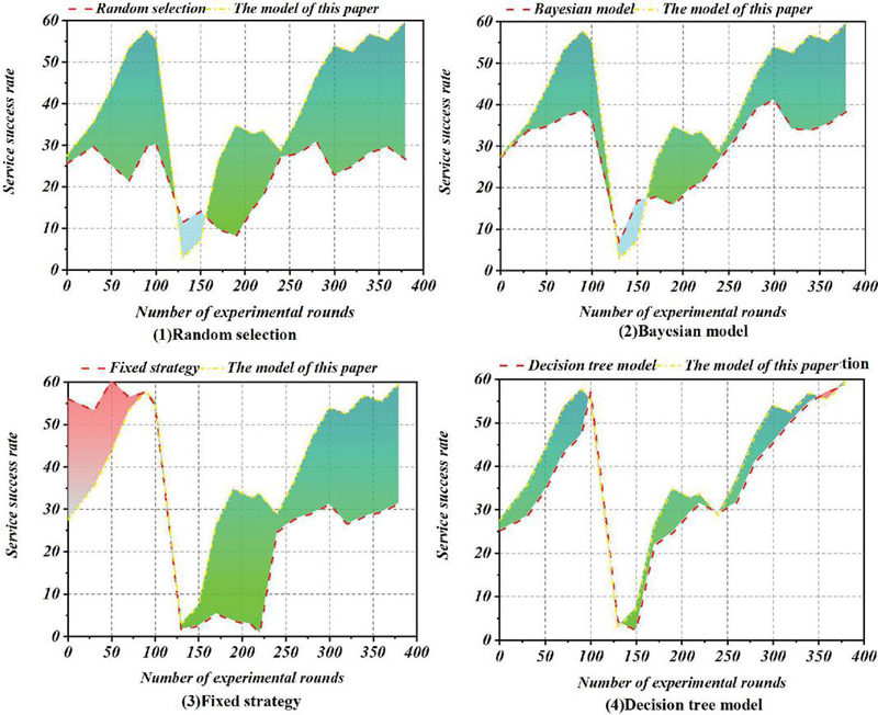
Figure 7 Experiments in dynamic network environment.
In the results of Experiment 3, the results of the stochastic model vary completely with the network conditions, and we omit it from the experimental results. The results of the Bayesian model are similar but with a slightly higher success rate. The fixed-policy model, which simulates a manually set policy, performs better in 1120 rounds of operation, reflecting the effectiveness of human intervention in executing a policy that is correctly set using experience. However, when there is a large-scale change in the network conditions, if it is not detected in time and manual intervention is made to update the policy, the execution effect is even worse than the random model. This point shows that when there are large-scale dynamic changes in the environment, most of the existing trust models using fixed policies or formulas and parameters cannot effectively adapt to this situation. Both the decision tree-based model and the model in this paper can effectively adapt to the changes that occur in the network environment. From the experimental data, the randomly generated rule set in this paper’s model tends to stabilize its evolution after 60 to 80 rounds of operation, with a high success rate; after a large-scale change in the network environment, the success rate drops to the level of the random selection method. However, without human intervention, the rule set evolves to a stable state again at 180200 rounds of operation, and the success rate still improves considerably; after 240 rounds of operation, the network environment is restored to the initial state, and the model still evolves to a high level again, although the roles of some nodes are changed.
4 Conclusion
With the increasing size of the network, network attacks, and sabotage behaviors are increasing day by day, and network security problems are becoming more and more prominent. Based on the clustering mechanism, this paper proposes a dynamic continuous trust assessment model and applies this model to the network security model optimization problem.
(1) The problems in the previous clustering algorithms are analysed, and corresponding solutions are proposed for the problems. Then the particle swarm algorithm is briefly introduced, the inertia weight coefficients in the particle swarm algorithm are improved, and the dormant mechanism of neighbouring node groups is introduced. On this basis, the optimal number of cluster heads of the network is re-analyzed.
(2) A new algorithm for calculating the direct trust value is proposed. Since the influence of the time factor on the calculation of trust value is not fully considered in the DyTrust trust model, this paper, in order to make the evaluation of the trust value of nodes more scientific and accurate, improves the algorithm used for calculating the direct trust value, and introduces the time decay factor w into the model, thus proposing a new algorithm used for calculating the direct trust value to achieve the distance from the current The distance from the present moment is inversely proportional to the influence of service satisfaction on the trust value, i.e., the closer to the present moment the greater the influence of service satisfaction on the trust value, and vice versa, the smaller the influence, increasing the accuracy of trust evaluation.
(3) An evaluation method for the overall trust value rating of the network is proposed. The method first selects the N nodes with the highest number of interactions, and then evaluates the overall trust level of the network where these N nodes are located by using the associative memory ability of the clustering algorithm.
(4) The experimental analysis shows that the randomly generated rule set in the model of this paper tends to be stable in evolution after 60 to 80 rounds of operation, with a high success rate; after a large-scale change in the network environment, the success rate drops to the level of the random selection method. However, without manual intervention, the rule set evolves to a stable state again at 180200 rounds of operation, and the success rate still improves considerably; after 240 rounds of operation, the network environment is restored to the initial state, and the model still evolves to a high level again, even though the roles of some of the nodes have changed. The model is able to adapt to the dynamic changes in the network environment by allowing entities to autonomously adjust their own trust assessment strategies to comprehensively assess each attribute of the entity without the manual involvement of the administrator.
References
[1] Liang Hua, Li Yang, Lei Juan, et al., 2022, Research on the evaluation method of Internet of Things nodes based on fuzzy evidence theory[J]. Journal of Southwest Normal University(Natural Science Edition), 47(03):111–124. DOI: 10.13718/j.cnki.xsxb.2022.03.013.
[2] Li Huanhuan, Xu Xiaoyun, Wang Honglei, 2021, Research on the architecture and application of network security model based on zero trust[J]. Science and Technology Information, 19(17):7–9. DOI: 10.16661/j.cnki.1672-3791.2107-5042-9133.
[3] Li Jinhua, Wang Hu, Lei Jianjun, 2019, Trust assessment model based on entropy weight method in trusted networks[J]. Journal of Central China Normal University (Natural Science Edition), 53(01):26–29. DOI: 10.19603/j.cnki.1000-1190.2019.01.005.
[4] Liu He, Wang Wei-Ying, Zhang Benli, 2014, Heterogeneous wireless network security model based on trust and risk assessment[J]. Journal of Heilongjiang Engineering Institute, 2014, 28(06):40–44. DOI: 10.19352/j.cnki.issn1671-4679.2014.06.011.
[5] Sinaga, K. P., and Yang, M. S. (2020). Unsupervised K-means clustering algorithm. IEEE Access, 8, 80716–80727.
[6] Xu, D., and Tian, Y. (2015). A comprehensive survey of clustering algorithms. Annals of data science, 2, 165–193.
[7] Dhanachandra, N., Manglem, K., and Chanu, Y. J. (2015). Image segmentation using the K-means clustering algorithm and subtractive clustering algorithm. Procedia Computer Science, 54, 764–771.
[8] Yuan, C., and Yang, H. (2019). Research on the K-value selection method of the K-means clustering algorithm. J, 2(2), 226–235.
[9] Nayak, J., Naik, B., and Behera, H. (2015). Fuzzy C-means (FCM) clustering algorithm: a decade review from 2000 to 2014. In Computational Intelligence in Data Mining-Volume 2: Proceedings of the International Conference on CIDM, 133–149.
[10] Yuan, G., Sun, P., Zhao, J., Li, D., and Wang, C. (2017). A review of moving object trajectory clustering algorithms. Artificial Intelligence Review, 47, 123–144.
[11] El Alami, H., and Najid, A. (2017). Fuzzy logic-based clustering algorithm for wireless sensor networks. International Journal of Fuzzy System Applications (IJFSA), 6(4), 63–82.
[12] Zhang, D., Ge, H., Zhang, T., Cui, Y. Y., Liu, X., and Mao, G. (2018). New multi-hop clustering algorithm for vehicular ad hoc networks. IEEE Transactions on Intelligent Transportation Systems, 20(4), 1517–1530.
[13] Murtagh, F., and Contreras, P. (2017). Algorithms for hierarchical clustering: an overview, II. Wiley Interdisciplinary Reviews: Data Mining and Knowledge Discovery, 7(6), 1219.
[14] Wang, D., Tan, D., and Liu, L. (2018). Particle swarm optimization algorithm: an overview. Soft computing, 22(2), 387–408.
[15] Piotrowski, A. P., Napiorkowski, J. J., and Piotrowska, A. E. (2020). Population size in particle swarm optimization. Swarm and Evolutionary Computation, 58, 100718.
[16] Ali, A. F., and Tawhid, M. A. (2017). A hybrid particle swarm optimization and genetic algorithm with population partitioning for large-scale optimization problems. Ain Shams Engineering Journal, 8(2), 191–206.
[17] Zhou, F. H., and Liao, Z. Z. (2013). A particle swarm optimization algorithm. Applied Mechanics and Materials, 303, 1369–1372.
[18] Juneja, M., and Nagar, S. K. (2016, October). Particle swarm optimization algorithm and its parameters: A review. In 2016 International Conference on Control, Computing, Communication and Materials (ICCCCM), 1–5.
[19] Lynn, N., Ali, M. Z., and Suganthan, P. N. (2018). Population topologies for particle swarm optimization and differential evolution. Swarm and evolutionary computation, 39, 24–35.
[20] Zhang, D., Ma, G., Deng, Z., Wang, Q., Zhang, G., and Zhou, W. (2022). A self-adaptive gradient-based particle swarm optimization algorithm with dynamic population topology. Applied Soft Computing, 130, 109660.
[21] Nayak, P., and Devulapalli, A. (2015). A fuzzy logic-based clustering algorithm for WSN to extend the network lifetime. IEEE Sensors Journal, 16(1), 137–144.
[22] Bures, T., Hnetynka, P., Heinrich, R., Seifermann, S., and Walter, M. (2020). Capturing dynamicity and uncertainty in security and trust via situational patterns. In Leveraging Applications of Formal Methods, Verification and Validation: Engineering Principles: 9th International Symposium on Leveraging Applications of Formal Methods, 9, 295–310.
[23] De Visser, E. J., Peeters, M. M., Jung, M. F., Kohn, S., Shaw, T. H., Pak, R., and Neerincx, M. A. (2020). Towards a theory of longitudinal trust calibration in human-robot teams. International journal of social robotics, 12(2), 459–478.
[24] Stavroulaki, V., Strinati, E. C., Carrez, F., Carlinet, Y., Maman, M., Draskovic, D., … and Demestichas, P. (2021). DEDICAT 6G-Dynamic coverage extension and distributed intelligence for human-centric applications with assured security, privacy, and trust: From 5G to 6G. In 2021 Joint European Conference on Networks and Communications & 6G Summit (EuCNC/6G Summit), 556–561.
[25] Ling Xiangrong (2023), Based on attention neural network and Bayesian optimization [D]. Xidian University. DOI: 10.27389/d.cnki.gxadu.2023.001113.
Biographies
Weidong Wu, Graduated from Central China University of Science and Engineering in 2003, currently employed at State Grid Hunan Electric Power Company Limited ChangSha, Research interests include Network Information Security and Applications.
Zheng Tian, Graduated from South China University of Technology in 2007, currently employed at Information and communication branch of State Grid Hunan Electric Power Company, Research interests include Network Information Security and Applications.
Yizhen Sun, graduated from Jiangxi University of Science and Technology in 2016, majoring in Computer Science and Technology. currently employed at Information and communication branch of State Grid Hunan Electric Power Company, Research interests include Network Information Security and Applications.
Youfa Li, graduated from Jiangxi University of Science and Technology in 2020, majoring in Computer Science and Technology. currently employed at Information and communication branch of State Grid Hunan Electric Power Company, Research interests include Network Information Security and Applications.
Yu Cui, Graduated from Beijing Foreign Study University in 2020, currently a Regional Manager at State Grid Informationn & Telecommunication Group CO., LTD, with a research focus on Computer Science and Technology.
Journal of Cyber Security and Mobility, Vol. 14_1, 47–74.
doi: 10.13052/jcsm2245-1439.1413
© 2025 River Publishers