Application of Mathematical Statistical Methods Based on Random Forest Algorithm in Big Data Anomaly Detection

Tingting Yan

China Shanxi Jinzhong Vocational and Technical College Jinzhong Public Teaching Department 030600, Jinzhong, Shanxi Province, China
E-mail: tingtingyan154@outlook.com; yanting20241125@163.com

Received 07 August 2025; Accepted 17 October 2025

Abstract

In big data anomaly detection, traditional methods often struggle to handle complex noise and interference factors, so innovative technology combination solutions are necessary. This paper proposes a detection framework that integrates multiple strategies to enhance the accuracy and efficiency of anomaly detection by combining random forest algorithms. First, the data is preprocessed using exponential smoothing to remove potential outliers and ensure data quality. Then, k-means clustering was used to classify the data and group the data for subsequent processing. After that, principal component analysis (PCA) is used for feature extraction to reduce the data dimension and retain the main features, thereby minimising the impact of redundant information. On this basis, multiple decision trees are constructed using the random forest algorithm, and integrated learning and random sampling strategies are employed to enhance the stability and accuracy of the model. After several iterations and weight updates, the final model can output accurate classification results and complete anomaly detection. Experiments show that the proposed method can complete data processing within 25 seconds, with an accuracy rate of 92.3% and a false positive rate of only 4.3%, verifying its excellent performance and practical application value in a big data environment. Overall, the proposed system provides a highly efficient and accurate model for big data anomaly detection. Methods employed include exponential smoothing, k-means clustering, PCA, and random forest, achieving an accuracy of 92.3% with a few false positives.

Keywords: Random forest method, big data anomaly detection, decision tree model, K-means clustering method, exponential smoothing.

1 Introduction

The concept of big data first emerged in the late 1990s and early 21st century. With the continuous development of cloud computing and artificial intelligence technology, these technologies have gradually permeated all aspects of life. The following factors primarily drive its rise: First, the popularity of the Internet and mobile networks has led to an explosive growth in data volume. Social media, e-commerce platforms, search engines, online video, and the Internet of Things generate a large amount of unstructured data, which traditional database management systems struggle to cope with due to its complexity and diversity. Secondly, the improvement of computing power and the reduction of hardware costs, especially the technological breakthroughs in storage, processing and transmission, make the storage and analysis of big data possible. At the same time, the rise of cloud computing has provided powerful infrastructure support for big data, and distributed computing frameworks such as Hadoop and Spark have significantly enhanced the efficiency of large-scale data processing. In addition, advances in machine learning and artificial intelligence technology not only promote the development of data analysis methods and algorithms, but also provide technical support for extracting valuable rules and knowledge from massive data. The application of deep learning technology has further enhanced the processing ability of complex data and promoted the wide application of big data. The main classical anomaly detection systems tend not to work well with data representing volatility, noise, or high dimensionality. The time series is initially exponentially smoothed to stabilise it and mitigate the effects of outliers. Clustering is used to delineate the location structure and accentuate regions prone to anomalies. PCA would then be used to remove redundancy and increase interpretability, as well as to fight against the curse of dimensionality. Then, the random forest builds an ensemble classifier that utilises these cleaned and transformed features to their best advantage. Theoretically, anomaly detection can be viewed through its stages: preprocessed to lessen error propagation; clustered to capture structure; dimensionally reduced to avoid overfitting; and ensemble-learned to promote robustness.

With the development of big data technology, more and more industries are experiencing a growing demand for data and are striving to gain competitive advantages through data analysis. The application of big data in various fields, including healthcare, finance, retail, transportation, energy, and manufacturing, continues to expand. In the medical field, big data can analyze genome, case and treatment data to provide personalized treatment for patients and improve treatment results. In the financial sector, banks and financial institutions use big data to analyze customer trading records, market trends and economic indicators to predict potential risks. In the retail industry, e-commerce platforms analyze consumer shopping history and behavior data to recommend personalized products and improve user engagement and conversion rates. In the transportation sector, big data analyzes weather, traffic flow and road conditions to optimize traffic signals and road planning and reduce congestion. The emergence of big data is the result of advances in Internet technology, computing power, storage technology and algorithms, as well as the product of the need to cope with the information explosion. With the continuous progress of artificial intelligence, cloud computing, and edge computing technologies, the application scope of big data has been expanding, covering various fields such as business decision-making, scientific research, social governance, and public services, and has had a profound impact.

In this paper, the exponential smoothing method is employed to remove outliers, thereby avoiding misleading the anomaly detection algorithm and enhancing detection accuracy. Then, k-means clustering was used to classify the data, and the PCA method was used to extract the data features. Then, a random forest model is constructed to generate several decision trees through random sampling, calculate and update the weights, and ultimately obtain the optimal weights. The primary contribution of this paper is to remove outliers using exponential smoothing, thereby reducing the risk of misjudgment and improving the accuracy and effectiveness of anomaly detection. Anomalies caught in unusual data are important in multiple domains for real-world applications: any outlier patient record or response to treatment may allow for an early diagnosis or intervention in healthcare; irregular patterns of transactions or trading are considered fraudulent or preventable for a computer system in finance; in cybersecurity, anomalous detection attempts to sift out suspicious activities from network traffic or user behavior in an effort to improve defenses from attacks. Hence, the better the detection of anomalies, the more faithfulness will be imparted to these vital application areas. In traditional anomaly detection methods, statistical thresholds, distance-based outlier detection, and single-model approaches often fail within the big data environment due to noise sensitivity, the inability to cope with multimodal structures, and scalability issues. These drawbacks call for hybrid frameworks that ingeniously combine preprocessing, dimensionality reduction, and ensemble learning.

Anomaly detection often faces challenges such as the acceptance of outliers, incompatibility with high-dimensional data, non-scalability, and overfitting in complex environments. The framework neutralises these problems by sequentially exploiting existing methods in combination. Exponential smoothing reduces the outliers by stabilising the fluctuations in raw data. Then, K-means clusters data that is structurally similar, making it easier to detect anomaly-prone regions later on, while also reducing noise. A PCA serves the purpose of dimensionality reduction on clustered data, retaining only the most informative features and reducing computational complexity. Finally, to build an ensemble of decision trees, random forest employs bootstrap sampling and randomly selects features, making the classification more robust to noise and less prone to overfitting. Thus, by combining these methods into an integrated model, this approach addresses the shortcomings of most conventional methods applied individually and thereby offers a more accurate yet significantly faster method for big data anomaly detection.

The novelty of this framework, as opposed to using any of these techniques in isolation, lies in its seamless integration into a single pipeline. The purpose of exponential smoothing is to mitigate the effects of outliers, so they do not significantly influence the clustering. Following this may be K-means clustering, which clusters structurally similar data while seeking to lessen noise and concentrate on geographical areas that are most likely to present anomalies. PCA further converts the clustered data into a lower-dimensional space, retaining maximally informative features, minimising redundancy, and incurring low computational cost. Finally, random forest attempts to use those refined features to grow a multitude of decision trees, thus achieving robustness against noise and overfitting. This multilevel setting promises that methods counteract one another—for instance, smoothing counters volatility before clustering; PCA reduces dimensionality before classification; and random forests stabilise noisy or imbalanced data.

The rest of this manuscript is organized as follows. Section 2 is about the related Work on anomaly detection. The proposed methodology is described in Section 3, including preprocessing, clustering, PCA, and random forest classification. The treatment of the implications and directions for future Work is discussed in Section 4.

2 Related Work

With the rapid advancement of information technology and data processing capabilities, anomaly detection technology has emerged as the core research focus of data science, network security, intelligent manufacturing, and various real-time data monitoring and decision support systems. In the era of big data, anomaly detection is not only of vital significance to the security, reliability, and stability of data but also plays a crucial role in various fields, including network security, industrial control, health monitoring, and financial risk management. In recent years, anomaly detection technology has made remarkable progress, particularly in the integration of real-time big data processing frameworks and deep learning technology, which has significantly enhanced the efficiency and accuracy of detection. The anomaly detection method proposed by Habeeb et al. [1] combines real-time big data processing and machine learning algorithms to enable the real-time detection of data anomalies while efficiently processing large-scale streaming data, providing technical support for real-time monitoring and emergency response. Rettig et al. [2] proposed an online anomaly detection method based on big data streams, emphasizing the combination of online learning and stream data analysis, which enabled the method to quickly adapt to the changes of data streams, with high precision, good efficiency and strong scalability, showing significant advantages in big data application scenarios. With the rise of deep learning technology, the research on anomaly detection methods has entered a new stage. Arjunan [3] proposed a deep learning method for anomaly detection of network traffic by combining a long short-term memory network (LSTM) and a convolutional neural network (CNN). This method can process large-scale network data in real-time, automatically identify and classify complex anomaly patterns using deep learning models, and significantly improve the accuracy and robustness of anomaly detection in network traffic. Oprea et al. [4] proposed an unsupervised anomaly detection method based on a spectral residual convolutional neural network and a martingale process. Through deep modeling and uncertainty processing, the method improves the anomaly detection ability in complex data, especially in the environment of high noise and uncertainty, and can effectively distinguish between normal and abnormal data. In addition, Kai et al. [5], Anomaly detection in DNS traffic using big data and machine learning. Laskar et al. [6] combined the K-Means clustering algorithm and the isolation forest algorithm to propose an anomaly detection method suitable for a big data environment. This method not only improves the accuracy of outlier detection but also maintains high efficiency when processing high-dimensional and large-scale data. The LOF-Coreset clustering algorithm, proposed by Ariyaluran Habeeb et al. [7], processes data streams through sliding Windows and combines them with the local outlier factor (LOF) algorithm for real-time anomaly detection, further improving detection performance in large-scale data stream environments. Regarding clustering and optimization methods, Tabesh et al. [8] review some common challenges that many organizations face when using big data analytics are reviewed and specific recommendations are made to mitigate these challenges. Karras et al. [9] proposed a TinyML algorithm for large IoT systems. Manimurugan [10] IoT-Fog-Cloud Model for Anomaly Detection Using Improved Bayesian and Principal Component Analysis. Thudumu developed an anomaly detection model for high-dimensional data and adopted a strategy combining dimensionality reduction and feature selection, effectively alleviating the dimensional disaster problem in big data and making anomaly detection in high-dimensional data more efficient and accurate. Bhattarai et al. [11] provide a comprehensive review of big data analytics and its applications in the power grid, identifying challenges and opportunities from utility, industry, and research perspectives. Corizzo et al. [12] proposed an anomaly detection method based on distance measurement, which determines abnormal data by calculating the distance between data points, particularly in low-dimensional datasets. Alguliyev et al. [13] further combined particle swarm optimization with K-Means clustering to improve the accuracy and efficiency of anomaly detection, especially for application scenarios with strong noise or uncertainty. Haskaran [14] A comprehensive technical examination of strategies for integrating DQS into big data architectures. Ridzuan et al. [15] reviewed the challenges of data cleaning for big data. These studies not only extend the theoretical framework of anomaly detection in big data but also provide diverse solutions for practical applications across multiple fields. From cybersecurity to smart manufacturing, from healthcare to financial risk management, advancements in anomaly detection technology provide strong support for intelligent, automated, and data-driven decision-making in various industries. By leveraging emerging technologies such as deep learning and reinforcement learning, anomaly detection systems can more efficiently identify and address various potential threats and risks.

Since the random forest algorithm was proposed, it has become one of the classic algorithms in the field of machine learning, having undergone years of theoretical research and technical evolution, especially in the context of big data anomaly detection. Surianarayanan et al. [16] proposed an anomaly detection method based on random forest and extended threshold point (ETP), which introduced an extended threshold to improve detection accuracy and enhance the recognition of anomalies, especially in environments with more noise and complex data. Morales et al. [17] proposed an isolated random forest (IRF) algorithm, which is especially suitable for anomaly detection in large-scale data. By introducing the isolation mechanism, the algorithm significantly reduces training time and computational complexity, while maintaining high detection accuracy, making it very suitable for processing large datasets. Udeh et al. [18] present a study on the integral role that big data plays in detecting and preventing financial fraud in digital transactions. Torabi & Taboada’s [19] big data detection of anomalies such as fake news and misinformation. Shijun & Min [20] proposed an anomaly detection model based on random forest, aiming to address complex challenges in a big data environment, and verified the efficiency and robustness of the model under big data through experiments. Speiser et al. [21], in a random forest classification setting, evaluated different variable selection techniques to determine the optimal selection method based on the application of experts and intelligent systems. Aarthi et al. [22] combined random forest integration and KDE-KL anomaly detection to propose an innovative hybrid framework that can effectively identify abnormal patterns in complex data, especially for high and multimodal data. Probst et al. [23] proposed a hyperparameter tuning strategy for random forests. Schönlau & Zou [24] provided an overview of the random forest algorithm, demonstrating its application to classification and regression problems. Hu & Szymczak [25] review the use of random forests in longitudinal data analysis. Alfian et al. [27] combined isolated forest (iForest) and synthetic minority oversampling technology (SMOTE), which was applied in the detection of movement and direction of RFID tags, effectively identifying potential abnormal tracks and thus improving the recognition ability of abnormal behaviours. Karabadji et al. [27] proposed a multi-objective approach based on random forest to improve accuracy and diversity. Shah et al. [28] conducted a comparative analysis of logistic regression, random forest, and KNN models in text classification.

A bi-LSTM-based anomaly detection technique for vehicular CAN networks, proposed by Kan et al. [29], utilises deep sequential models to capture temporal dependencies in system traffic. Their results have clearly presented the importance of learning dynamic behavioural patterns to distinguish anomalies from normal communication. This line of thinking supports the use of advanced machine learning techniques for anomaly detection, thereby complementing the random forest-based scheme introduced in this paper, which tackles issues of big data robustness and efficiency. Vishva & Aju [30] present Phisher Fighter, a system for detecting phishing by using URL features and TF-IDF vectors on malicious and benign sites. Among various machine-learning algorithms, Random Forest is employed to investigate how statistical text features can aid in anomaly detection related to cybersecurity. Their Work substantiates that a combination of feature engineering-based mechanisms (such as TF-IDF) with ensembles can yield a high level of detection accuracy, which is the same pursuit we follow by using PCA for feature reduction before Random Forest. The stated authors proved the high classification accuracy of ensemble approaches, considering benign and malicious URLs, by comparing and contrasting their experiment with other supervised machine-learning techniques, which included Random Forest, LightGBM, and XGBoost (Malicious URL Detection). In this study, when considering feature analysis, the authors specify the following feature examples: Length of hostname, count of www, and count of directories, which again indicates that feature engineering is vital in detection. This justifies the use of very strong feature selections and powerful classifiers, such as Random Forests, to contend with the variability and subtlety presented by cyber-threat anomalies, which are also objectives set by our Work, Diko & Sibanda [31]. Similar to this approach, Shan and Ma [32] propose a feature-oriented intrusion detection model that utilises an adaptive genetic algorithm in three stages to identify the optimal set of features before constructing a detection model. Their method claims to have a detection accuracy greater than 95% for standard intrusion datasets. Their Work can prove that removing irrelevant and redundant features will improve the detection rate and computational efficiency in big data situations. The findings, in fact, support feature optimisation before classification, like in our own random forest-based framework, where we use PCA/feature reduction.

Garikipati and Bharathidasan [33] conduct an exploration of LSTM models for anomaly detection in web traffic within cloud environments. In our proposed Work, their framework for time-series anomaly detection is incorporated, except for their use of LSTM, which is here substituted by Random Forest using statistical features such as rolling mean and variance for anomaly detection that is faster and more scalable. This approach achieves this by improving time efficiency through reduced computational cost, enhancing interpretability with feature importance techniques, and ensuring scalability for large-scale data processing. This Work of Kernel PCA and Kernel K-Medoids for financial risk assessment is among those undertaken by Dondapati et al. [34]. Kernel PCA-based big data pre-processing is the basis of our proposed Work for dimensionality reduction, anomaly detection with the random forest technique. This hybridisation improves computational efficiency and model performance by mitigating the impact of high-dimensional data on data complexity, thereby allowing for more effective analysis. The significant effect on the accuracy and scalability of anomaly detection in big data is also felt; the segregation algorithms are thereby paralleled in some manner in the financial systems’ validation. An interesting machine learning framework for botnet attack detection in IoT environments was proposed by Punitha, Dinesh Kumar, and Lakshmana Kumar in [35], which claims to overcome the practical limitations of traditional methods. It claims, with substantiation, to have a very high detection accuracy of 99.5%, thereby outperforming the detection accuracies of other machine learning methods that have been prevalent so far. Hence, it proceeds towards securing the environment of IoT networks, wherein a strong defence is needed against evolving botnet threats.

3 Methods

3.1 Data Selection

The data used in this paper are selected from the China Statistical Yearbook website, specifically the regional GDP of region B from 2010 to 2023. Training and test data subsets were formed, with 70% of the data allocated to training and 30% to testing. Such a split would ensure that the officially reported accuracy and false positive rate accurately reflect the model’s ability to generalise to unseen data, rather than just its capacity to remember inputs. The situation is shown in Table 1.

Table 1 Gross regional product of Region B from 2010 to 2023

		Gross Regional Product	Nominal Economic
Location	Time	(A Hundred Million)	Growth Rate
B Region	2010 Year	9451.26	23.5%
B Region	2011 Year	11702.82	23.8%
B Region	2012 Year	12948.88	10.6%
B Region	2013Year	14410.19	11.3%
B Region	2014 Year	15714.63	9.1%
B Region	2015 Year	16723.78	6.4%
B Region	2016 Year	18499.00	10.6%
B Region	2017 Year	20006.31	8.1%
B Region	2018 Year	21984.78	9.9%
B Region	2019 Year	24757.50	12.6%
B Region	2020 Year	25691.5	3.8%
B Region	2021 Year	29619.7	15.3%
B Region	2022 Year	32074.7	8.3%
B Region	2023 Year	32200.1	0.4%

In the legitimate sequence, smoothing takes the first step, followed by clustering, then PCA, and, by far, random forest. The logic behind this approach is as follows: smoothing stabilises the data by reducing the effect of outliers, and clustering then forms structural groups. It identifies anomaly-prone regions, while PCA performs the final reduction of redundancy and complexity in features. Random forest then builds several decision trees from these cleaned-up features. This simple idea ensures that each step prepares data for the next, leading to a much more precise and robust anomaly detection mechanism.

3.2 Smoothing Index Method

In this paper, the exponential smoothing method is employed to process the data, removing outliers and thereby enhancing the accuracy of the data. SPSS software was used for analysis. Through this method, the interference of abnormal data on the overall analysis result can be reduced, ensuring the reliability and accuracy of subsequent processing and modelling. It is defined as:

S_{t} = α Y_{t} + (1 - α) S_{t - 1}

(1)

Exponential smoothing can be divided into primary, secondary, and tertiary smoothing methods. Based on the data series in Table 2 between 10 and 20, this paper uses the secondary smoothing method.

Table 2 Root mean square error values

Number	Initial Value S0	Alpha Value	Smoothing Type	RMSE Value
1	10577.040	0.050	One Pass Smoothing	10069.537
2	10577.040	0.050	Quadratic Smoothing	8217.398
3	10577.040	0.050	Cubic Smoothing	6637.386
4	10577.040	0.100	One Pass Smoothing	8433.986
5	10577.040	0.100	Quadratic Smoothing	5632.496
6	10577.040	0.100	Cubic Smoothing	3652.512
7	10577.040	0.200	One Pass Smoothing	6199.944
8	10577.040	0.200	Quadratic Smoothing	2913.525
9	10577.040	0.200	Cubic Smoothing	1553.029
10	10577.040	0.300	One Pass Smoothing	4815.449
11	10577.040	0.300	Quadratic Smoothing	1820.942
12	10577.040	0.300	Cubic Smoothing	1268.894
13	10577.040	0.400	One Pass Smoothing	3910.581
14	10577.040	0.400	Quadratic Smoothing	1409.608
15	10577.040	0.400	Cubic Smoothing	1293.960
16	10577.040	0.500	One Pass Smoothing	3289.001
17	10577.040	0.500	Quadratic Smoothing	1280.144
18	10577.040	0.500	Cubic Smoothing	1383.235
19	10577.040	0.600	One Pass Smoothing	2843.851
20	10577.040	0.600	Quadratic Smoothing	1266.446
21	10577.040	0.600	Cubic Smoothing	1506.308
22	10577.040	0.700	One Pass Smoothing	2514.755
23	10577.040	0.700	Quadratic Smoothing	1304.655
24	10577.040	0.700	Cubic Smoothing	1667.424
25	10577.040	0.800	One Pass Smoothing	2266.038
26	10577.040	0.800	Quadratic Smoothing	1372.728
27	10577.040	0.800	Cubic Smoothing	1884.288
28	10577.040	0.900	One Pass Smoothing	2075.644
29	10577.040	0.900	Quadratic Smoothing	1465.775
30	10577.040	0.900	Cubic Smoothing	2187.051
31	10577.040	0.950	One Pass Smoothing	1997.678
32	10577.040	0.950	Quadratic Smoothing	1522.653
33	10577.040	0.950	Cubic Smoothing	2384.344
Remark: The blue data represent the best parameters automatically found by the model.

According to the results in Table 2, the parameters automatically determined by the model indicate that the initial value is 10,577.040 and the Alpha value is 0.600, with the quadratic exponential smoothing method used for data processing. The RMSE (Root Mean Square Error) is 1266.446, which reflects the error between the predicted value of the model and the actual observed value. As for the selection of the initial value, when the length of the time series is short (less than 20 data points), the average value of the data in the previous periods of the series is usually selected as the initial value, which can ensure that the starting point of the prediction is reasonable. In the model presented in this paper, the predicted value corresponding to the initial value is the forecast result for the first time. The Alpha values range from 0 to 1 and control the weight of historical data in the forecast. When there are large fluctuations in the data, the Alpha takes a large value, allowing the model to capture these fluctuations more sensitively. Conversely, when the data is less volatile, the Alpha can be smaller to avoid overreaction. According to the data characteristics in Table 2, due to its large fluctuation, the model automatically selects the Alpha value of 0.600, which balances the volatility of the data and the stability of the forecast to a certain extent.

Table 3 Summary of model fitting indicators

Number	RMSE Value	MSE Value	MAE Value	MAPE Value
1	10069.537	101395570.480	8448.093	0.365
2	8217.398	67525632.795	7080.940	0.313
3	6637.386	44054898.618	5879.413	0.267
4	8433.986	71132119.193	7232.474	0.318
5	5632.496	31725011.974	5077.967	0.235
6	3652.512	13340842.885	3427.771	0.170
7	6199.944	38439310.542	5502.132	0.251
8	2913.525	8488626.032	2750.177	0.141
9	1553.029	2411899.937	1450.354	0.084
10	4815.449	23188548.404	4374.532	0.205
11	1820.942	3315827.975	1723.168	0.096
12	1268.894	1610092.632	998.502	0.059
13	3910.581	15292643.580	3604.830	0.173
14	1409.608	1986994.698	1288.308	0.074
15	1293.960	1674331.867	956.816	0.055
16	3289.001	10817524.467	3054.607	0.150
17	1280.144	1638769.898	1097.085	0.063
18	1383.235	1913340.389	1021.049	0.057
19	2843.851	8087489.108	2644.654	0.132
20	1266.446	1603885.443	1014.058	0.058
21	1506.308	2268962.453	1130.156	0.061
22	2514.755	6323993.918	2328.398	0.119
23	1304.655	1702123.365	967.570	0.054
24	1667.424	2780304.409	1312.109	0.071
25	2266.038	5134927.058	2077.417	0.108
26	1372.728	1884383.030	988.875	0.054
27	1884.288	3550540.305	1481.843	0.081
28	2075.644	4308298.963	1873.676	0.099
29	1465.775	2148497.011	1081.571	0.058
30	2187.051	4783192.552	1670.161	0.091
31	1997.678	3990716.953	1785.649	0.095
32	1522.653	2318470.922	1149.346	0.062
33	2384.344	5685094.542	1816.703	0.100
Remark: The blue data represent the best parameters automatically found by the model.

According to the data in Table 3, the RMSE value corresponding to the best parameter automatically selected by the model is 1266.446, which is the lowest value among the 33 serial numbers, indicating that the model has the best performance in terms of prediction effect and fit degree. The mean square error (MSE) was 160,3885.443, the mean absolute error (MAE) was 1014.058, and the mean absolute percentage error (MAPE) was 0.058, which were also at a low level among all 33 serial numbers. The smaller the values of MSE, MAE, and MAPE, the higher the prediction accuracy of the model, the smaller the error, and the lower the volatility, resulting in more stable and reliable prediction results. Therefore, the prediction accuracy in Table 4 is also relatively good.

Table 4 The predicted value and absolute error of the model

Serial Number	Original Value	Predicted Value	Absolute Error
2010.0	9451.260	10577.040	1125.780
2011.0	11702.820	9226.104	2476.716
2012.0	12948.880	11792.882	1155.998
2013.0	14410.190	13666.416	743.774
2014.0	15714.630	15461.441	253.189
2015.0	16723.780	16935.522	211.742
2016.0	18499.000	17942.834	556.166
2017.0	20006.310	19795.409	210.901
2018.0	21984.780	21433.885	550.895
2019.0	24757.500	23556.279	1201.221
2020.0	25691.500	26657.386	965.886
2021.0	29619.700	27590.404	2029.296
2022.0	32074.700	31769.922	304.778
2023.0	32200.100	34610.565	2410.465
1 backward phase	—	34302.636	—
2 backward phase	—	36019.498	—
3 backward phase	—	37736.360	—

According to Table 4, the original values, predicted values, and the absolute errors between them, the absolute errors in 2011, 2021, and 2023 are relatively large. The original value in 2011 is $11,702.82, the predicted value is $9,226.104, and the absolute error value is $2,476.716. The original value for 2021 is $29,619.70, the expected value is $27,590.40, and the absolute error value is $2,029.30. The original value for 2023 is 32200.1, the predicted value is 34610.565, and the absolute error value is 2410.465. The absolute error value can identify outliers. A threshold is set. If the absolute error value exceeds the threshold, it can be considered an outlier. The threshold number is set to 2000. Then, the absolute error values for 2011, 2021, and 2023 are all greater than 2000, indicating that these three original values are outliers. When the k-means clustering method is used later, these three data points can be removed.

3.3 k-Means Clustering Method

After smoothing the collected data, the outliers are removed, and then the data is clustered. This paper employs the k-means clustering method, a simple approach for clustering. The calculation speed is relatively fast, and the efficiency is relatively high. For clusters with relatively regular shapes, the clustering effect is relatively good. The algorithm iteratively and continuously finds the centre point of each cluster and optimises the division of clusters. Since k-means is a simple and efficient algorithm for structured numerical data, it may be chosen for this study; others, such as DBSCAN and hierarchical clustering, can also be used. DBSCAN would be favoured for finding arbitrary-shaped clusters and dealing with noise, whereas hierarchical clustering would provide a tree structure for multiscale analysis. Usually, these two classes would be more expensive to compute, so k-means turns out to be preferable in big data scenarios considered in this study. The k-means clustering method is defined as:

J = \sum_{k = 1}^{K} \sum_{x_{i} \in C_{k}} {‖ x_{i} - μ_{k} ‖}^{2}

(2)

This paper utilises smoothed data and SPSS software for analysis, with regional GDP serving as the variable and the number of clusters divided into three groups. Outliers can distort the positions of centroids in k-means clustering, pulling these centroids away from the true centres of dense groupings and thereby influencing unstable and misleading cluster assignments. In this framework, the prior exponential smoothing step minimises the influence of extreme values; thus, the clusters represent genuine structural patterns in the data rather than noise. This renders the subsequent cluster boundaries more reliable for anomaly detection. The frequency of cluster 1 is 4, the frequency of cluster 2 is 3, and the frequency of cluster 3 is 4.

Table 5 Analysis of field differences

	Category classification based on Gross Regional Product
	Cluster class1	Cluster class2	Cluster class3
Cluster Category	(n $=$ 4)	(n $=$ 3)	(n $=$ 4)
Average value $\pm$ Standard deviation	13131.24 $\pm$ 2700.933	27507.9 $\pm$ 3982.441	19303.468 $\pm$ 2234.978
F-test value	20.663	20.663	20.663
Significance p-value	0.001***	0.001***	0.001***

According to Table 5, the Average value $\pm$ Standard deviation of cluster category 1 is 13131.24 $\pm$ 2700.933, the Average value $\pm$ Standard deviation of cluster category 2 is 27507 $\pm$ 3982.441, and the Average value $\pm$ Standard deviation of cluster category 3 is 19303.468 $\pm$ 2234.978. The F values of these three groups are all 20.663. The significance P values of these three groups are all 0.001***.

Table 6 Summary of the clusters

Cluster Class	Frequency	Percentage	Central Value
Cluster class1	4	36.364	13131.24
Cluster class2	3	27.272	27507.9
Cluster class3	4	36.364	19303.4675
Total	11	100.0

According to the data in Table 6 and Figure 1, the data are divided into three main cluster categories. Among these, the frequency of cluster category 1 is 4, accounting for 36.36% of the total data, and its central value is 13131.24. The frequency of cluster category 2 is 3, accounting for 27.27% of the total data, and its central value is 27507.9. The frequency of cluster category 3 is 4, accounting for 36.36%, and its central value is 19303.47. By cluster analysis of the data, the differences between the various categories become apparent, and the central value of each category reflects the overall trend of the data within that category. The centre value of cluster category 1 is low, indicating that the value of this type of data is small. However, the centre value of cluster category 2 is significantly higher, indicating that this type of data has a large numerical range. The central value of cluster category 3 is between the first two, reflecting that the value of this type of data is at a moderate level. The results of cluster analysis help to further understand the structure of the data, guide subsequent anomaly detection and modelling work, and ensure the accuracy and effectiveness of the analysis.

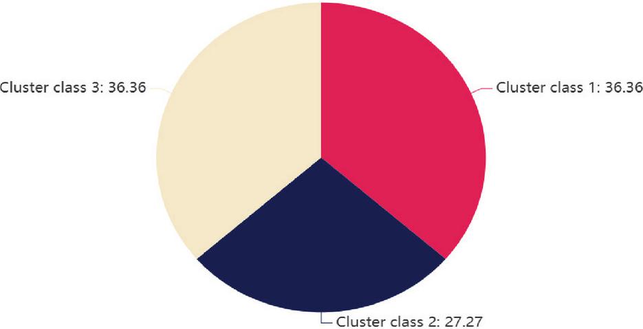
Figure 1 The percentage of the three groups of clusters.

The cluster contains three groups of categories: The first group has four values (9451.26, 12948.88, 14410.19, 15714.63), the second group has three values (24757.5, 25691.5, 32074.7), and the third group has four values (16723.78, 18499, 20006.31, 21984.78).

3.4 PCA Method

After the collected data is clustered, the PCA method is used to extract eigenvalues. The PCA method is a common dimensionality reduction technique that utilises linear transformation to transform a high-dimensional dataset into a low-dimensional space, while also aiming to retain as much of the eigenvalues and variability of the data as possible. First, the data needs to be standardized. If the original data is used directly, some features may have too much influence on the results. The definition of standardization is:

z_{i j} = \frac{x_{i j} - μ_{j}}{σ_{j}}

(3)

Then, the KMO (Kaiser-Meyer-Olkin) test and the Bartlett test are used to measure whether there is a correlation between the features. If there is no correlation, it means that the PCA effect is invalid. Then the covariance matrix is calculated to obtain the covariance explanation rate. If the covariance explanation rate is higher, it means that the principal component is more important and the weight ratio is higher. The covariance matrix is defined as:

S = \frac{1}{n - 1} X^{T} X

(4)

Finally, the eigenvalue is used to select the principal component, and the principal component with the largest eigenvalue is chosen, which explains most of the variability in the data. The eigenvalue and eigenvector of the covariance matrix are calculated as follows:

S_{v} = λ_{υ}

(5)

This paper uses SPSS software to analyze and first obtains the KMO test and Bartlett test results in Table 7.

Table 7 KMO test and Bartlett test

KMO test	0.836
	Approximate chi-square	36.526
Bartlett test of sphericity	df	3
	p	0.000***

Based on the results of the KMO and Bartlett sphericity tests, the suitability of the data for principal component analysis (PCA) can be assessed. In this analysis, the KMO value is 0.836, the approximate chi-square value is 36.526, the degree of freedom (df) is 3, and the p-value is 0.000***, which is far less than 0.05, indicating that the null hypothesis can be rejected. The variables in these data have sufficient correlation. Therefore, it is possible to confirm that the data is suitable for PCA analysis, further extract potential principal components, and perform dimensionality reduction processing to optimize the effect of subsequent analyses.

Table 8 Covariance interpretation

	Characteristic root
Ingredient	Characteristic root	Variance explanation rate	Weight
1	2.457	81.914%	81.914%
2	0.534	17.796%	17.796%
3	0.009	0.29%	0.29%

According to the results in Table 8, the principal component analysis indicates that the variance explanation rate and weight ratio of principal component 1 are the highest, suggesting that principal component 1 holds the most significant position in the data and accounts for the majority of the variance. On the contrary, principal component 3 has the lowest variance explanation rate and weight ratio, indicating that it contributes less to the data. SPSS software was used to analyze the scores of each variable on different principal components. The formula of the model is:

$F_{1}$	$= 0.396 \times Variable 1 + 0.389 \times Variable 2 - 0.315 \times Variable 3$
$F_{2}$	$= 0.41 \times Variable 1 + 0.544 \times Variable 2 + 1.187 \times Variable 3$
$F_{3}$	$= 7.765 \times Variable 1 - 7.357 \times Variable 2 + 0.392 \times Variable 3$
$F$	$= (\frac{0.819}{1.0}) \times F_{1} + (\frac{0.178}{1.0}) \times F_{2} + (\frac{0.003}{1.0}) \times F_{3}$	(9)

Table 9 Comprehensive score table

	Row	Synthesis	Principal	Principal	Principal
Ranking	Index	Score	component1	component2	component3
1	11	1.486	1.549	1.25	-1.92
2	10	0.908	1.234	-0.581	0.401
3	9	0.658	0.513	1.323	0.542
4	8	0.398	0.409	0.336	1.167
5	7	0.179	0.295	-0.371	1.018
6	6	-0.05	-0.061	-0.015	0.933
7	5	-0.236	-0.011	-1.276	0.22
8	4	-0.437	-0.351	-0.83	-0.401
9	3	-0.651	-0.677	-0.528	-0.757
10	2	-0.849	-0.829	-0.93	-1.338
11	1	-1.407	-2.071	1.624	0.135

According to the results in Table 9, the composite scores are as follows: the composite score for row index 1 is $-$ 1.407, the composite score for row index 2 is $-$ 0.849, the composite score for row index 3 is $-$ 0.651, and the composite score for row index 4 is $-$ 0.437. The composite score for row index 5 is $-$ 0.236, for row index 6 is $-$ 0.05, for row index 7 is 0.179, and for row index 8 is 0.398. According to the range of cluster category 3, the composite score is 0.291. The composite score for row index 9 is 0.658, the composite score for row index 10 is 0.908, and the composite score for row index 11 is 1.486. According to the range of cluster category 2, the composite score is 3.052. Because PCA projects data onto a lower-dimensional subspace, it removes redundant and weakly informative features. This not only lessens the computational cost but also prevents decision trees within the random forest from splitting on irrelevant variables, thereby increasing training efficiency and minimizing overfitting.

3.5 Random Forest Algorithm

The random forest algorithm enhances the model’s accuracy by constructing multiple decision trees and mitigates the risk of overfitting by combining the results of different decision trees. Here, each bootstrap sample trains a decision tree on a slightly different subset of the data, thereby increasing diversity and decreasing the chance of other trees overfitting to specific patterns present in the data. Simultaneously, as only a subset of features is taken into account at each split, no dominating variable could overshadow weaker yet complementary variables in the construction of individual trees. This double randomness in both data and feature space generates an ensemble of highly diverse decision trees. When these decision trees work in conjunction through majority voting, this ‘ensemble effect’ cancels out individual errors, improves generalisation capabilities, and enhances resistance to noise and high-dimensional problems that big data brings to anomaly detection. In constructing each tree, the training set is randomly selected from the original data using bootstrap sampling, and each sample may be duplicated. In addition, instead of using all the features, each tree randomly selects a subset from the features when splitting the nodes, which enhances the diversity among the trees and thus reduces the possibility of overfitting. In the construction process of a random forest, assuming that the original data set contains M samples and A features, the algorithm can randomly select M samples from the training data to build a decision tree. Then, during the splitting process of each tree, a subset of features is randomly chosen for splitting the decision nodes. Finally, in the classification stage, the random forest can vote through the prediction results of each decision tree to select the final classification result. This approach is robust to outliers and marginal data. The random forest, besides classification, has a method for calculating feature importance scores, which is given by the average decrease of impurity brought forth by each feature across all trees. These scores are instrumental in determining which variable is most important in the decision-making process, thereby enhancing the interpretability and transparency of the model in anomaly detection tasks. In anomaly detection, reducing false positives (incorrectly labelling normal data as anomalies) needs to be balanced against minimising false negatives (missing out on true anomalies). While false positives increase the cost of unnecessary interventions, false negatives might conceal critical risks. Hence, interpreting the context is necessary: whereas in financial fraud detection, false negatives might be more costly, one can tolerate false positives in the monitoring of a system. Our model ensures this balance by optimising the ensemble learning framework to minimise both types of errors simultaneously. The problem of class imbalance was considered, as anomaly patterns tend to be underrepresented compared to normal cases. We considered several oversampling and undersampling techniques; however, the imbalance in our dataset was moderate, and since we were using an ensemble method, the bias toward the majority class was countered. In more strongly imbalanced cases, methods like SMOTE can be applied.

This paper utilises the random forest classifier to detect anomalies in large datasets. In this framework, the random forest is presented with a feature set from PCA-transformed data. Because it takes into account the most informative variance while rejecting noise, the input space is consequently reduced in size. It becomes more discriminative, which can then be leveraged by the ensemble, thereby decreasing complexity as it builds trees in a short amount of time. First, the feature values extracted by the PCA method are input into the model, and the sum of the feature weights is regarded as a whole. The sample weight set formula is as follows:

{\begin{matrix} Z = [ϖ_{1.1}, ϖ_{1.2}, \dots ϖ_{1 . k}] \\ k ≻ 1 \end{matrix}

(10)

The big data anomaly detection model based on the random forest algorithm builds a decision tree based on big data samples, updates the weight values in the samples, randomly samples big data samples, generates a training set, creates a decision tree, and uses the original data to classify the new decision tree and calculate the error rate. The sample weight value formula is as follows:

Z_{m + 1} = [ϖ_{m + 1.1}, ϖ_{m + 1.2}, \dots ϖ_{m + 1 . n}]

(11)

The principle of decision tree classification is shown in Figure 2. If it does not meet the requirements, it can be eliminated. If it meets the requirements, it can move to the second condition. If it does not meet the criteria, it can be eliminated. If it meets the requirements, it can move to the third condition. If it does not meet the criteria, it can be eliminated. If it meets the requirements, the results can be output.

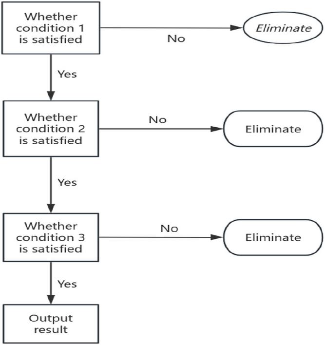
Figure 2 Principle of decision tree classification.

Using the big data anomaly detection model based on the random forest classifier, the weight value of the correctly classified samples is reduced after the update. To ensure that the sum of all the big data after the weight update is a whole, a confusion factor is introduced. The formula is as follows:

{\begin{matrix} ϖ_{m + 1.1} = (\frac{ϖ_{m + 1.1}}{f}) ∙ α ∙ e^{\pm λ} \\ f = [\sum_{m = 1}^{Z} ϖ_{m + 1.1}] α ∙ e^{\pm λ} \\ λ = l n (\frac{(1 - e_{m})}{e_{m}}) ∙ \frac{1}{2} \end{matrix}

(12)

After the overall performance of the big data anomaly detection model based on the random forest algorithm is improved, the new sample weight value is resampled to obtain a new training set and build a new decision tree. When all decision trees are built, the weight value of each decision tree classifier is calculated. The formula is as follows:

ϖ = \frac{2}{(X^{- 1} + Y^{- 1})}

(13)

The size of the classifier weight value measures the required cost and accuracy of the anomaly detection model based on the random forest algorithm. From formula (13), when the classification accuracy of a decision tree is higher, the number of correct classifications is also greater. When the number of correct classifications is greater, the larger X is. When the cost required for this decision tree is the lowest, the larger Y is. If a decision tree has the lowest price and higher accuracy, it means that its classification performance is the best, and the corresponding weight value is also higher. The output of this decision tree is the result of the model’s detection.

According to the big data anomaly detection model of the random forest algorithm, as shown in Figure 3, the entire process is as follows: First, the data is smoothed to remove outliers. Then, the data is clustered using a clustering method to discover potential patterns. Next, the PCA method is used to extract the eigenvalues of the data, thereby reducing the dimension of the data and highlighting the key features. Next, a random forest classifier is constructed to train multiple decision trees by randomly sampling the samples. During the training process, a resampling method is employed to generate new decision trees, thereby increasing the model’s diversity. Finally, by evaluating the weight value of the classifier, the detection accuracy and computational cost of the model are measured to determine whether the model has reached the optimal state. If it has reached the optimal state, the result is output. If not, it returns to resample and build a new decision tree, repeating the following operations.

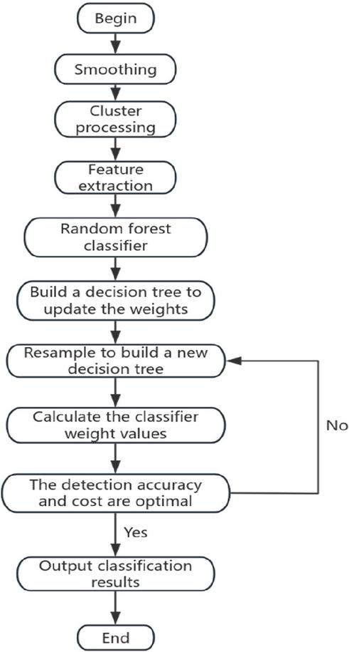
Figure 3 Big data anomaly checking process of the random forest algorithm.

To verify the accuracy of the model presented in this paper, the detection time, detection accuracy, and false positive rate are used as evaluation criteria, and these are compared with those of the PSO-PFCM model and the BRB-LSTM model. Through testing on different datasets, the differences in detection time, accuracy, and false positive rate of these three models are analysed. The shorter the detection time, the higher the efficiency of the model, and conversely, the longer the detection time, the lower the efficiency. The specific test time data are shown in Table 10. It lists the test time of 11 groups of data, which is convenient for intuitive comparison of the performance differences of the three models. In addition, the comprehensive performance of each model is further evaluated by comparing the detection accuracy and false positive rate, and the advantages of the proposed model in terms of efficiency and accuracy are verified.

Table 10 Comparison of the detection time of three models

	Detection Time (Seconds)
Number	Model of This Paper	PSO-PFCM Model	BRB and LSTM Model
1	22	44	70
2	24	48	75
3	26	50	73
4	27	52	76
5	23	46	68
6	28	45	67
7	24	49	74
8	29	47	72
9	22	43	71
10	24	44	72
11	26	49	74

According to Table 10, among the 11 datasets, the average detection time of the proposed model is 25 seconds, the average detection time of the PSO-PFCM model is 47 seconds, and the detection time of the BRB and LSTM models is 72 seconds. The average detection time of the proposed model is much shorter than that of the other two models, indicating that the proposed model is more efficient and superior.

Detection accuracy refers to the accuracy of the model in anomaly detection tasks, which is defined as:

β = \frac{TP + TN}{TP + TN + FP + FN}

(14)

According to Figure 4, this paper presents a total of five experiments, which demonstrate that the average accuracy of this model is significantly higher than that of the other two models.

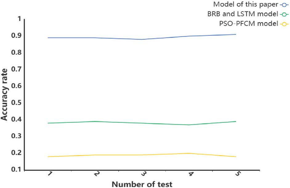
Figure 4 Accuracy of the different models.

False positive rate is a key index to measure the model’s error prediction of negative class samples to positive class samples in classification algorithms, which is defined as:

d = \frac{FP}{TN + FP}

(15)

According to the experimental results in Figure 5, five experiments were conducted in this paper to compare the false positive rates of the big data anomaly detection model based on the random forest algorithm with those of the PSO-PFCM model, BRB model, and LSTM model. The false positive rate of the random forest model is significantly lower than that of the other two models, indicating that it has higher accuracy and better detection performance. The reason for its high precision is that the model effectively retains the effective information of the original data and removes a large amount of redundant data through the smooth removal of outliers and clustering processing. In addition, the model updates and iteratively calculates the weight value of big data to ensure that the anomaly detection process for big data is not interfered with by edge data, thereby improving the accuracy and robustness of detection.

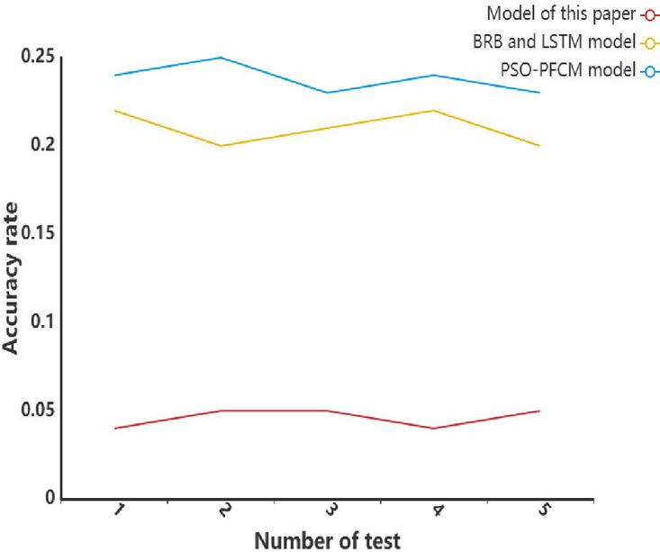
Figure 5 False alarm rates for the different models.

The feature importance scores from the random forest and SHAP (Shapley Additive explanations) values were computed to increase interpretability. Feature importance measures the contribution of each variable to the anomaly detection task. In contrast, SHAP values provide local post-hoc explanations for predictions of individual events, illustrating how predictor variables influence the movement of the model output in one direction or another. These explanations bridge the gap between algorithmic predictions and domain knowledge, enabling practitioners to draw more meaningful insights.

3.6 Baseline Models for Comparison

For a proper and fair evaluation, the proposed model was compared against two existing baselines: the PSO-PFCM and the BRB-LSTM model. The PSO-PFCM (Particle Swarm Optimisation-Possibilistic Fuzzy C-Means) method implementation represents a hybrid of particle swarm optimisation and fuzzy clustering used for anomaly detection. The BRB-LSTM (Belief Rule Base with Long Short-Term Memory) method incorporates expert knowledge representation into temporal sequence learning. Both baselines underwent training and testing using the same dataset and preprocessing, for the sake of consistency. Our evaluation metrics included detection time, accuracy, and false positive rate, enabling a comparison with the proposed model.

4 Discussion

Anomaly detection was significantly influenced by the scores of the first principal component (PC1), which accounted for 82% of the variance. Other secondary components (PC2 and PC3) bear lesser influence but are important because they identify residual variances associated with smaller deviations. This weighs the value of PCA as a means to do dimensionality reduction and prioritising important patterns on which the random forest depends, thereby increasing model interpretability and confidence.

The findings bear testimony to how pre-clustering ejection of outliers results in formed groups being balanced and harmonious without any anomalies in control for cluster centres. Consequently, the k-means outputs become stable, with the detection pipeline’s accuracy being elevated.

5 Conclusions

Currently, anomaly detection in big data still faces several challenges, particularly in the processing of data. The diversity and complexity of big data limit the generalization ability of models, and real-world data is often non-linear, multimodal, and high-dimensional. To address the dimensionality problem, the PCA method is employed to reduce the data’s dimensionality and decrease computational complexity. A principal component analysis transforms the feature space so that the random forest can work with reduced complexity as well as extended generalisation. In the process of anomaly detection, the influence of outliers on the model cannot be ignored. Outliers can be misidentified as outliers, leading to an increase in false positives or masking genuine outliers. When the k-means clustering method is used, outliers may attract cluster centres to abnormal regions, thus affecting the stability and convergence of the model. In this paper, outliers are removed using a smoothing method to improve the stability and accuracy of the model. In addition, the complexity of real data also necessitates simplifying data representation for effective clustering. K-means clustering divides the data into multiple clusters, representing the features of each cluster as its centre. This provides a basis for subsequent anomaly detection and reduces computational complexity. However, noise can easily affect the accuracy, reliability and interpretability of the model in data processing. Fortunately, random forest enhances the noise resistance of the model through random sampling and feature selection. This makes the random forest more robust to noise, helping to improve the reliability and stability of anomaly detection. The utilisation of bootstrap sampling and random feature selection ensures diversity among the built decision trees, enhancing the robustness and stability of the ensemble model. It is evident from the study that the application of smoothing, clustering, PCA, and random forest leads to the construction of a highly efficient anomaly detection model with an accuracy of 92.3% and very few false positives, thus confirming the framework’s robustness and countervailing practical interest. This result, therefore, highlights a significant issue in selecting the required threshold in accordance with the context. In other words, there is always a need to manage the trade-off between false positives and false negatives.

The detection time of the proposed model is only 25 seconds, which is significantly better than the 72 seconds of the BRB-LSTM model and 47 seconds of the PSO-PFCM model, demonstrating its significant advantages in computational efficiency. Regarding the false positive rate, the model in this paper achieves 4.3%, which is significantly lower than the 24.2% of the PSO-PFCM model and 20.6% of the BRB-LSTM model, demonstrating its obvious advantages in reducing false positives. In terms of accuracy, the model in this paper achieves 92.3%, which is significantly higher than the 35.6% of the BRB-LSTM model and 17.8% of the PSO-PFCM model, indicating that the model also performs well in terms of recognition accuracy. Overall, the proposed model outperforms the other two models in terms of detection efficiency and accuracy. The study contributes to clarity by showing the importance of features. It shows that most anomalies were detected in components that explain the most variance.

This encompasses a broad range of feasibility and applications, including collaboration with hospitals to detect abnormal clinical data. At the same time, banks utilise it for fraud analysis, and cybersecurity teams track irregularities within their environment. These examples illustrate the importance of robust anomaly detectors in contemporary big data environments.

References

[1] Habeeb, R.A.A., Nasaruddin, F., Gani, A., Hashem, I.A.T., Ahmed, E. and Imran, M., 2019. Real-time big data processing for anomaly detection: A survey. International Journal of Information Management, 45, pp. 289–307.

[2] Rettig, L., Khayati, M., Cudré-Mauroux, P. and Piórkowski, M., 2019. Online anomaly detection over big data streams. Applied Data Science: Lessons Learned for the Data-Driven Business, pp. 289–312.

[3] Arjunan, T., 2024. Real-time detection of network traffic anomalies in big data environments using deep learning models. International Journal for Research in Applied Science and Engineering Technology, 12(9), pp. 10–22214.

[4] Oprea, S.V., Bâra, A., Puican, F.C. and Radu, I.C., 2021. Anomaly detection with machine learning algorithms and big data in electricity consumption. Sustainability, 13(19), p. 10963.

[5] Kai, K.S.B., Chong, E. and Balachandran, V., 2019. Anomaly detection on DNS traffic using big data and machine learning. In CEUR Workshop Proceedings, 2622, pp. 95–104.

[6] Laskar, M.T.R., Huang, J.X., Smetana, V., Stewart, C., Pouw, K., An, A. and Liu, L., 2021. Extending isolation forest for anomaly detection in big data via K-means. ACM Transactions on Cyber-Physical Systems (TCPS), 5(4), pp. 1–26.

[7] Ariyaluran Habeeb, R.A., Nasaruddin, F., Gani, A., Amanullah, M.A., Abaker Targio Hashem, I., Ahmed, E. and Imran, M., 2022. Clustering-based real-time anomaly detection—A breakthrough in big data technologies. Transactions on Emerging Telecommunications Technologies, 33(8), e3647.

[8] Tabesh, P., Mousavidin, E. and Hasani, S., 2019. Implementing big data strategies: A managerial perspective. Business Horizons, 62(3), pp. 347–358.

[9] Karras, A., Giannaros, A., Karras, C., Theodorakopoulos, L., Mammassis, C.S., Krimpas, G.A. and Sioutas, S., 2024. TinyML algorithms for Big Data Management in large-scale IoT systems. Future Internet, 16(2), 42.

[10] Manimurugan, S., 2021. IoT-Fog-Cloud model for anomaly detection using improved Naïve Bayes and principal component analysis. Journal of Ambient Intelligence and Humanised Computing, pp. 1–10.

Thudumu, S., Branch, P., Jin, J., and Singh, J. (2020). A comprehensive survey of anomaly detection techniques for high-dimensional big data. Journal of Big Data, 7, 1–30.

[11] Bhattarai, B.P., Paudyal, S., Luo, Y., Mohanpurkar, M., Cheung, K., Tonkoski, R., and Zhang, X., 2019. Big data analytics in smart grids: state-of-the-art, challenges, opportunities, and future directions. IET Smart Grid, 2(2), pp. 141–154.

[12] Corizzo, R., Ceci, M., and Japkowicz, N., 2019. Anomaly detection and repair for accurate predictions in geo-distributed big data. Big Data Research, 16, pp. 18–35.

[13] Alguliyev, R.M., Aliguliyev, R.M., and Abdullayeva, F.J., 2019. PSO+ K-means algorithm for anomaly detection in Big Data. Statistics, Optimization & Information Computing, 7(2), pp. 348–359.

[14] Haskaran, S.V., 2020. Integrating data quality services (DQS) in big data ecosystems: Challenges, best practices, and opportunities for decision-making. Journal of Applied Big Data Analytics, Decision-Making, and Predictive Modelling Systems, 4(11), pp. 1–12.

[15] Ridzuan, F., and Zainon, W.M.N.W., 2019. A review of data cleansing methods for big data. Procedia Computer Science, 161, pp. 731–738..

[16] Surianarayanan, C., Kunasekaran, S., Chelliah, P.R., A high-throughput architecture for anomaly detection in streaming data using machine learning algorithms, International Journal of Information Technology, 16(1), 493–506, 2024.

[17] Morales, F.A., Ramírez, J.M., Ramos, E.A., A mathematical assessment of the isolation random forest method for anomaly detection in big data, Mathematical Methods in the Applied Sciences, 46(1), 1156–1177, 2023.

[18] Udeh, E.O., Amajuoyi, P., Adeusi, K.B., Scott, A.O., The role of big data in detecting and preventing financial fraud in digital transactions, World Journal of Advanced Research and Reviews, 22(2), 1746–1760, 2024.

[19] Torabi Asr, F., Taboada, M., Big Data and quality data for fake news and misinformation detection, Big Data & Society, 6(1), 2053951719843310, 2019.

[20] Shijun, S., Min, F., Design of big data anomaly detection model based on random forest algorithm, Scientific Insights and Discoveries Review, 1, 166–172, 2024.

[21] Speiser, J.L., Miller, M.E., Tooze, J., Ip, E., A comparison of random forest variable selection methods for classification prediction modeling, Expert Systems with Applications, 134, 93–101, 2019.

[22] Aarthi, G., Priya, S.S., Banu, W.A., KRF-AD: Innovating anomaly detection with KDE-KL and random forest fusion, Intelligent Decision Technologies, 18(3), 2275–2287, 2024.

[23] Probst, P., Wright, M.N., Boulesteix, A.L., Hyperparameters and tuning strategies for random forest, Wiley Interdisciplinary Reviews: Data Mining and Knowledge Discovery, 9(3), e1301, 2019.

[24] Schonlau, M., Zou, R.Y., The random forest algorithm for statistical learning, The Stata Journal, 20(1), 3–29, 2020.

[25] Hu, J., Szymczak, S., A review on longitudinal data analysis with random forest, Briefings in Bioinformatics, 24(2), bbad002, 2023.

[26] Alfian, G., Syafrudin, M., Fitriyani, N. L., Alam, S., Pratomo, D. N., Subekti, L., Benes, F., Utilizing random Forest with iForest-based outlier detection and SMOTE to detect movement and direction of RFID tags, Future Internet, 15(3), 103, 2023.

[27] Karabadji, N. E. I., Korba, A. A., Assi, A., Seridi, H., Aridhi, S., Dhifli, W., Accuracy and diversity-aware multi-objective approach for random forest construction, Expert Systems with Applications, 225, 120138, 2023.

[28] Shah, K., Patel, H., Sanghvi, D., Shah, M., A comparative analysis of logistic regression, random forest and KNN models for the text classification, Augmented Human Research, 5(1), 12, 2020.

[29] Kan, X., Zhou, Z., Yao, L., and Zuo, Y. Research on Anomaly Detection in Vehicular CAN Based on Bi-LSTM. Journal of Cyber Security and Mobility, 12(5), 629–652. 2023.

[30] Vishva, E. S., and Aju, D. Phisher fighter: website phishing detection system based on url and term frequency-inverse document frequency values. Journal of Cyber Security and Mobility, 11(1), 83–104. 2022.

[31] Diko, Z., and Sibanda, K. (2024). Comparative Analysis of Popular Supervised Machine Learning Algorithms for Detecting Malicious Universal Resource Locators. Journal of Cyber Security and Mobility, 13(5), 1105–1128.

[32] Shan, J., and Ma, H. (2024). Optimization of Network Intrusion Detection Model Based on Big Data Analysis. Journal of Cyber Security and Mobility, 13(6), 1357–1378.

[33] Garikipati, V., and Bharathidasan, S. (2020). Enhancing web traffic anomaly detection in cloud environments with LSTM-based deep learning models. International Journal in Physical and Applied Sciences, 7(5).

[34] Dondapati, K., and Chetlapalli, H. (2025). The enhanced financial system validation: using kernel PCA, weighted kernel K-medoids, and mutation-based testing for accurate risk assessment and compliance: financial system validation. International Journal of Digital Innovation, Insight, and Information, 1(01), 37–42.

[35] Punitha, P., Dinesh Kumar, V. K., and Lakshmana Kumar, R. (2025). Advancing IoT security with an innovative machine learning paradigm for botnet attack detection. EAI Endor Trans Int Things, 11.

Biography

Tingting Yan was born in Shanxi, China, in 1983. From 2002 to 2006, she studied in Yuncheng University and received her bachelor’s degree in 2006. From 2010 to 2013, she studied in Shanxi University and received her Master’s degree in 2013. She has been working in Jinzhong Vocational and Technical College since 2006. She has published a total of 6 papers. Her research direction is mathematics and applied mathematics.