Network Security Posture Assessment Algorithm Based on Multilayer Perceptron of Graph Convolutional Neural Networks
Xiaofeng Zhao1,*, Qianjun Wu2 and Peng Wang3
1Book and Information Center, Anhui University of Finance & Economics, Bengbu, 233030, China
2Bengbu City Card Limited Liability Company, Bengbu 233000, China
3Bengbu City Network Security Emergency Center, Bengbu 233000, China
E-mail: zhaoxf@aufe.edu.cn
*Corresponding Author
Received 16 September 2025; Accepted 13 December 2025
Abstract
With the increasing complexity and security threats in cyberspace, network security situation assessment has become a key technology to ensure digital security. This study proposes a hybrid model integrating graph convolutional neural networks and multi-layer perceptrons to address the limitations of traditional methods in capturing the topological associations of complex networks and dynamic threat responses. First, this model uses graph convolutional neural networks to aggregate node neighborhood information and capture topological features. Then, it conducts deep nonlinear feature learning through multi-layer perceptrons. Finally, it screens key information through pooling layers. Finally, the situation level assessment is achieved by the Softmax classifier. Experiments showed that the accuracy rates of the model on the CICIDS and UNSW-NB15 datasets reached 96.5% and 94.3% respectively, and its performance was superior to that of the comparison models. In the simulation and dynamic environment tests, the model evaluation results were stable, with an average evaluation time of only 66.19 ms and a resource utilization rate of 53.87%. The hybrid model constructed in this study effectively overcomes the challenges of feature fusion and classification in complex network environments. It provides a novel solution for efficiently and accurately assessing network security situations and has significant practical application value.
Keywords: NSSA, GCN, MLP, feature fusion, feature learning.
1 Introduction
The rapid development of internet technologies, such as cloud computing and 5G, has made cyberspace increasingly complex. It is now filled with large amounts of heterogeneous data, complex topologies, and dynamic threats [1]. Meanwhile, new attack techniques are constantly emerging, rendering traditional defense methods inadequate for dealing with the complex network security situation [2, 3]. Against this backdrop, the network security situation assessment (NSSA) urgently needs to be upgraded to be more multidimensional, dynamic, and intelligent. This has become a key research direction at present [4]. Cheng et al. established an assessment model based on evidence-based reasoning algorithm and belief rule base method for NSSA problem in the Internet. The outcomes revealed that this method not only could effectively utilize semi-quantitative information, but also solved the problem of uncertainty of different experts’ knowledge, and had strong applicability [5]. To improve the performance of a network security condition prediction model, Sun J et al. proposed a training method that combined model diagnostic meta-learning with bidirectional gated recurrent units. Experimental results showed that the model trained by this method improved the goodness-of-fit coefficient by 15.8%–18.1% compared to the traditional learning model [6]. To address the shortcomings of current NSSA techniques with regard to feature extraction (FE) and efficiency, Yu put out a unique fusion model. To provide important features the proper weights and increase the model’s accuracy, an attention mechanism was included. The model performed better in a number of assessment measures, according to experiments [7]. Wang et al. proposed a cyber security assessment model based on improved unsupervised learning clustering algorithm for cyberspace security. The model was tested experimentally with an accuracy of 99.83% and a running time of 0.27 s, which had good application results [8].
Graph convolutional neural networks (GCNs) are used to process graph-structured data by aggregating the information of neighboring nodes (NNs) to capture complex associated features in topological networks [9]. Because of its strong modeling capabilities for non-Euclidean data, it has been used extensively in fields including social networks, transportation networks, and cybersecurity in recent years. Yang H et al. proposed a GCN model incorporating multi-graph learning in order to predict the propagation flow in transportation networks. The model could capture temporal and spatial features simultaneously and effectively predict traffic propagation flow [10]. Reka et al. proposed a gated GCN model based on multi-head self-attention for recognizing multiple attack intrusions in cyberspace. The outcomes indicated that the model reduced the memory consumption of the intrusion detection system and maintained a higher attack recognition rate with less computation time [11]. Presekal et al. proposed a hybrid model using graphical convolutional long- and short-term memory and deep convolutional networks for the problem of recognizing power grid attack posture. The study’s findings demonstrated that the model outperformed time series classification techniques and could identify active assault areas [12]. To identify illicit Bitcoin trading transactions, Alarab I et al. suggested a hybrid optimization model that combines time series and GCN networks. According to the experimental findings, the suggested model’s accuracy under the identical circumstances was 97.77%, which was higher than that of earlier study models [13].
In conclusion, although significant progress has been made in existing research on complex network environments, effectively capturing topological correlations and achieving efficient dynamic threat responses remains challenging. In view of this, this study innovatively proposes a hybrid evaluation model that combines multi-layer perceptrons (MLP) with GCN. This model uses GCN’s neighbor aggregation mechanism to capture topological features and enhances node representations using MLP’s deep nonlinear transformation capabilities. The real-time optimization of the evaluation process is achieved through dynamic weight adjustment. This provides a brand-new solution that considers efficiency, accuracy, and adaptability when assessing the security situation of complex network environments. This approach explores a new technical path for improving the intelligence level of network security defense systems.
2 Methods and Materials
2.1 GCN-based NSS Element Construction and FE
Cybersecurity data has a natural graph structure as well as complex association relationships, which is a typical non-Euclidean data structure. Different from traditional convolutional neural networks and recurrent neural networks, GCN networks do not rely on the regular network structure, but define the convolution operation directly on the graph. GCN captures complex associated features in the network through the adjacency matrix (AM) and node information to achieve information aggregation and propagation. This feature makes it naturally suitable for dealing with the complexity of heterogeneous associations of cybersecurity data, the dynamics of risk level changes, and the coexistence of local and global associations [14]. The GCN structure is shown in Figure 1.
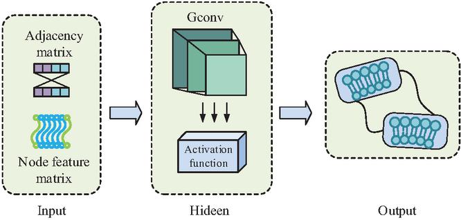
Figure 1 GCN structure (Source from: Author’s self drawn).
In Figure 1, the basic GCN result is mainly composed of three core parts, i.e., input layer (IL), hidden layer (HL), and output layer (OL). The IL receives the original graph data consisting of node feature matrices and neighbor matrices. The information of NNs is aggregated by graph convolution operation in the HL, and local information propagation is achieved through message passing mechanism. An activation function (AF) is introduced in each graph convolution layer to enhance the FE capability of the model. Finally, the final updated node feature information is output by the OL [15]. Equation (1) displays the graph convolution layer’s convolution formula.
| (1) |
In Equation (1), denotes the number of graph convolution layers. and denote the node features of the th and th layers, respectively. denotes the AF. denotes the weight matrix, which is used to map the node features activated by the AF to the new feature space. denotes the AM, which determines the NNs to be aggregated [16]. The AM is invariant during the information propagation process. Its formula is shown in Equation (2).
| (2) |
In Equation (2), denotes the dimension. is the unit matrix of dimension, which serves to add the self-loop to the AM. denotes the AM after adding the self-loop. denotes the transformation of the degree matrix . Its conversion formula is shown in Equation (3).
| (3) |
In Equation (3), and denote the nodes in row and column of the matrix, respectively. The information of each node is normalized by the degree matrix . Message passing neural network (MPNN) is a message passing mechanism in GCN network [17]. After the GCN graph convolutional layer captures the local features of the node data, the propagation of the graph node interconnection information and node update is accomplished through the MPNN mechanism. Among them, the MPNN structure of the convolutional layer is shown in Figure 2.
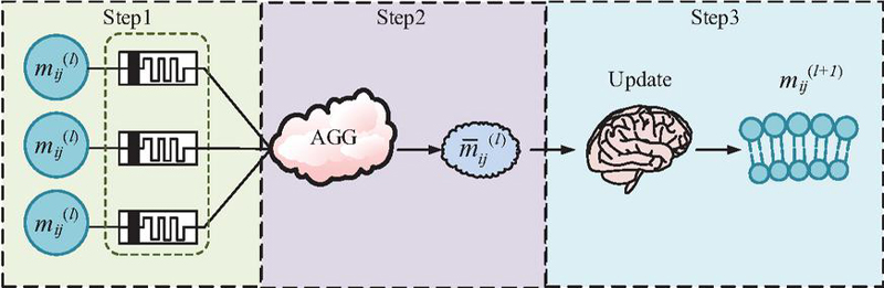
Figure 2 MPNN structure (Source from: Author’s self drawn).
In Figure 2, MPNN implements the feature learning of NSS through a hierarchical message passing mechanism. Its core computational process can be divided into three key phases, i.e., information generation, information aggregation, and information update. First, in the information generation phase each network security entity node collects information from its NNs and generates information containing threat semantics. Second, the information aggregation phase selectively aggregates neighboring information such as malicious attacks, vulnerabilities, traffic anomalies, etc., using the multi-head attention mechanism. Finally, in the information updating phase, the aggregated information is combined with the current state of the node to generate new node features through the gated updating mechanism. In this, Equation (4) displays the formula for the first step of information creation [18].
| (4) |
In Equation (4), denotes the message from node to node in layer . and denote the feature vectors (FVs) of the current node and the NN . denotes the edge feature between node and . denotes the learnable message function. The formula for the second step of neighbor message aggregation is shown in Equation (5).
| (5) |
In Equation (5), denotes the neighbor information of node after aggregation. is the set of NNs of node . denotes the aggregation function. The formula for the final information update is shown in Equation (6).
| (6) |
In Equation (6), denotes the post-update feature of node in layer. denotes the update function. Based on this, the study takes the information of devices, IP addresses, vulnerabilities, attack events, etc. in the network security data as the node information in GCN. The MPNN mechanism in GCN is used to aggregate the neighbor information to realize the security data in a certain network environment and perform security situation element construction and FE. The overall process is shown in Figure 3.
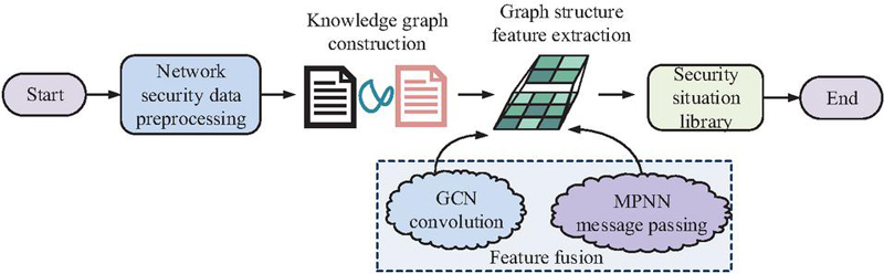
Figure 3 Security situation construction and FE flowchart (Source from: Author’s self drawn).
In Figure 3, the overall process of security situation element construction and FE realizes the conversion from raw network data to NSS knowledge graph through four main steps. The first is the data preprocessing stage. Multi-source data such as threats, firewalls, traffic probes, etc. in a certain network environment are taken as the source of network security data. To guarantee the data’s quality and consistency, it is cleansed, filled in, and normalized. Second, the preprocessed data related to NSS are filtered to construct a knowledge graph of NSS elements. Next, the network node features are taken using GCN, and the transfer, fusion, and extraction of graph structure features are accomplished through the MPNN mechanism. The processed node information is updated to enhance the knowledge base. Finally, the knowledge base of security situation elements is constructed for subsequent situation assessment.
2.2 NSSA Model Construction by Fusing MLP and GCN
The study constructs a basic model for NSS FE based on GCN neural network and its internal information transfer mechanism. Although GCN effectively captures topological association features through neighbor-joining aggregation, its ability to represent the intrinsic attributes of a single node is limited by the simplicity of linear transformations. Therefore, the research continues to improve it by introducing MLP, which utilizes its ability of nonlinear mapping to complement GCN. MLP neural network is a convolutional neural network-like structure derived from biological neurons. Its core mechanism is to enhance the representation of node information through nonlinear feature changes. It is able to provide GCN with node features that remove redundancy and have high differentiation, thus enhancing the detection accuracy of NSSA. It is suitable for the processing of network security data containing a large amount of irrelevant information [19]. Figure 4 depicts the MLP neural network’s fundamental architecture.
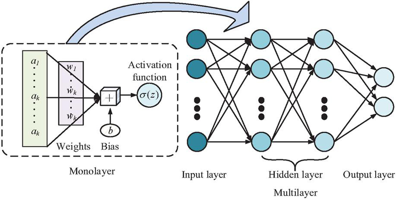
Figure 4 MLP structure (Source from: Author’s self drawn).
In Figure 4, the basic structure of the MLP neural network is composed of three main hierarchical parts, i.e., IL, HL, and OL. Each input node is connected to the first HL via a weighted connection, and the IL is in charge of receiving the original node FVs. Each layer of neurons in the HL performs deep feature learning on the input data and realizes nonlinear feature transformation through AFs. Finally, the enhanced node features are output through the OL. In this, the output formula of each neuron in each layer is shown in Equation (7) [20–22].
| (7) |
In Equation (7), is the activation value of the th neuron. denotes the AF. and are weights and bias. means the input. In this case, the error transfer calculation formula is shown in Equation (8).
| (8) |
In Equation (8), denotes the error value of HL . The formula of MLP neural network after passing the error is shown in Equation (9).
| (9) |
In Equation (9), denotes the learning update rate, which is used to control the update rate of weights and biases. In summary, MLP neural networks are introduced into the GCN model by utilizing their ability to learn features with enhanced node representations. The learning of each input node data by the model may be improved in this way. The final structure of the neural NSSA model fusing MLP and GCN is shown in Figure 5.
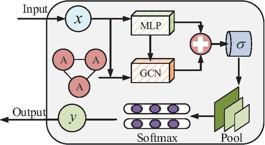
Figure 5 MLP-GCN assessment model (Source from: Author’s self drawn).
In Figure 5, the NSSA model fusing MLP and GCN can be divided into three stages: node feature learning, feature fusion, and classification evaluation. First, the GCN convolutional aggregation of NN graph data is utilized to achieve information dissemination and updating between each network posture element. Second, the updated and enhanced information representations are combined. The key data is retained by removing the interfering information after pooling. Finally, the evaluation results are output through classifier classification. The study adopts TopK pooling layer to select key graph data. The TopK pooling layer related formula is shown in Equation (13).
| (13) |
In Equation (13), denotes the node features of the final output. is the input vector. is the projection vector. is the Euclidean paradigm of the vector . denotes the scoring function. denotes the index of all nodes retained. denotes the retained node FV. denotes the element multiplication. denotes the normalized vector weights. Then all the retained node FVs are summed by summation pooling to get the global features of the graph. The formula for summation pooling is shown in Equation (14).
| (14) |
In Equation (14), denotes the result of additive pooling. denotes the number of nodes. denotes the FV of the th node. The global features of the graph are classified using Softmax classifier. Its formula is shown in Equation (15).
| (15) |
In Equation (15), denotes the input value of the th node. denotes the natural logarithmic exponential function taken. denotes the number of categorized species. In summary, the study uses a certain network environment as a data source to construct the overall flow of the NSSA algorithm that fuses MLP and GCN, as shown in Figure 6.
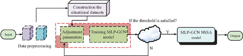
Figure 6 MLP-GCN NSSA flowchart (Source from: Author’s self drawn).
In Figure 6, the MLP-GCN model constructed by the study is roughly divided into four key steps. First, multi-source heterogeneous security data is sent to the system for preprocessing in an attempt to guarantee that the data quality satisfies the criteria for further analysis. Then, it enters the construction phase of the assessment system to determine the appropriate assessment indicators. The indicators are also quantified to construct an assessment dataset containing three dimensions: basic network performance, security threat level, and system vulnerability. Then, the initially constructed MLP-GCN model is trained to obtain the best combination of parameters and determine whether the model satisfies the threshold condition. If satisfied, the MLP-GCN assessment model is output. If it is not satisfied, return to the model training step and continue to iterate with parameter adjustment. Finally, the complete model with completed parameter adjustment is utilized for evaluation to obtain the final results.
3 Results
3.1 Performance Test of GCNNSSA Model with MLP Fusion
To validate the performance of the constructed model, an experimental environment with Intel Core i9-13900K CPU, NVDIA RTX 4090 GPU, 64GB DDR5 6400MHz RAM, and Windows 11 operating system is set up for the study. Canadian Institute for Cybersecurity Intrusion Detection Dataset (CICIDS) and University of New South Wales Network Security Centre Dataset (UNSW-NB15) are selected as the test datasets. CICIDS is a publicly available dataset provided by the Canadian Institute for Cyber Security Studies. It contains normal traffic and many common network attack techniques, and is a commonly used NSSA-specific dataset. UNSW-NB15 is also a classic intrusion test dataset suitable for comparative validation of model performance.
To ensure the reproducibility of the experiment and the fairness of the model evaluation, systematic preprocessing is carried out on the CICIDS and UNSW-NB15 datasets used in the study. First, data cleaning and filling are performed: For missing values in the dataset, they should be imputed using the mean value of the same feature column. Outliers with abnormal values or those that are clearly illogical should be removed. Next, feature encoding and normalization are required: For all categorical features that are not numerical types (such as protocol type, service type, etc.), they should be converted using the one-hot encoding method. For all numerical features, the min-max normalization method is adopted to linearly scale them to the interval [0, 1] to eliminate the influence of dimensions. Next, feature selection is carried out: The study calculates the correlations between all features and the target labels. Moreover, based on the feature importance calculated by the RF classifier, the top 50 most discriminative features are screened out to reduce the data dimension and remove redundant information. Then, the issue of class imbalance is addressed: Due to the uneven distribution of normal and attack traffic in the dataset, the study uses the SMOTE oversampling technique to synthesize minority class samples in the training set. This balances the volume of data in each category. Finally, the dataset is divided: The preprocessed complete dataset is randomly divided into a training set, a validation set, and a test set in a ratio of 70% : 15% : 15%. The training set is used to learn the model parameters. The validation set is used for hyperparameter tuning and early stopping. The test set is used to evaluate the model’s generalization performance.
The study first tests the selected values of two types of hyperparameters that affect the performance of the model, i.e., the number of HLs and the learning update rate of the MLP. Figure 7 displays the test findings.
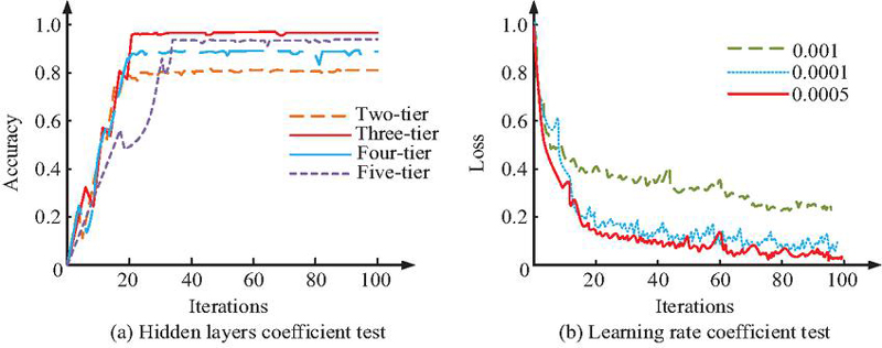
Figure 7 Two types of hyperparameter value testing.
In Figure 7(a), the accuracy comparison for the case of MLP neural network HL number of layers from 2 to 5. When the HL is 2, the model is able to iterate quickly to stability, but the accuracy is only 80.03% at the highest. When the HL is 4, the accuracy increases from 2, up to 86.17%. When the HL is 5, the accuracy is up to 96.55%. When the HL is 3, the accuracy of the model increases rapidly with the number of iterations and stabilizes. The accuracy reaches 99.52% after 100 iterations. Figure 7(b) represents the loss function comparison for different values of parameter learning update rate . When the update rate takes the value of 0.0005, the model loss function decreases rapidly with the increase in the iteration and stabilizes at a later stage. In summary, the study determines that the HL layers of the MLP neural network is 3 and the learning update rate is 0.0005. The parameter configuration of the MLP neural network model is optimal. The study continues by introducing three models that are more commonly used today to compare the performance of the models constructed for the study. These models include GCN, random forest (RF) and graph attention network (GAT). The test results are shown in Figure 8.
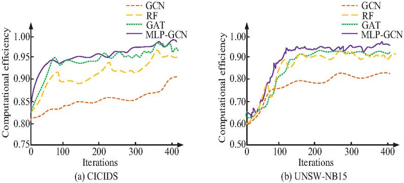
Figure 8 Accuracy test results.
Figure 8(a) represents the test outcomes on the CICIDS dataset. On the CICIDS dataset, the computational efficiencies of all four models show an increasing trend with the increase in the iteration. However, the single GCN model has the lowest computational efficiency (CE), with the highest CE of only 80.23%. The model proposed in the study has high CE at the early stage of operation. The CE increases rapidly with the increase in the iterations, and the highest CE is about 97.65%. Although the GAT model has high CE in the running process, it fluctuates more in the later stage. Figure 8(b) represents the test outcomes in the UNSW-NB15 dataset. In Figure 8(b), the research-proposed model also performs well in the UNSW-NB15 dataset with the highest CE of about 96.54%. To demonstrate the advantages of the model in a multi-dimensional way, the test is continued with accuracy, recall, and F1-score (F1) as the reference metrics. Table 1 displays the findings.
Table 1 The index test results of different model
| Data Set | Model | Accuracy/% | Recall/% | F1-score/% |
| CICIDS | GCN | 87.5 | 87.5 | 88.4 |
| RF | 92.1 | 90.5 | 91.1 | |
| GAT | 93.1 | 92.8 | 93.5 | |
| MLP-GCN | 96.5 | 95.7 | 96.4 | |
| UNSW-NB15 | GCN | 88.7 | 84.9 | 85.5 |
| RF | 91.3 | 89.7 | 89.9 | |
| GAT | 90.2 | 88.3 | 89.7 | |
| MLP-GCN | 94.3 | 94.1 | 93.8 |
In Table 1, the accuracy of the MLP-GCN model is 96.5% and 94.3% on the two types of datasets tested, which is significantly higher than the single GCN and RF models. The recall of MLP-GCN model on two types of datasets is 95.7% and 94.1%, respectively, which is about 2%–10% higher than the rest of the models. The F1 outperforms the other three models in every way, with respective scores of 93.8% and 96.4%. This result further validates that the proposed MLP-GCN model can model the assessment data using GCN and enhance the learning through MLP. It demonstrates superior performance in dealing with different cybersecurity datasets. To comprehensively and rigorously evaluate the model performance, in this study, each model is independently run 30 times on each dataset (using different random seeds). Moreover, its accuracy rate, recall rate and F1 are recorded. The arithmetic Mean and standard deviation of these operation results are calculated in the study, and the Paired t-test is used to analyze the statistical significance between the proposed MLP-GCN model and the performance indicators of each baseline model. A is considered statistically significant. The detailed results are shown in Table 2.
Table 2 Comparison of performance indicators of different models under multiple runs
| Dataset | Model | Accuracy (%) | Recall (%) | F1-score (%) |
| CICIDS | GCN | 87.21 0.84 | 86.95 1.12 | 87.89 0.91 |
| RF | 91.87 0.56 | 90.24 0.78 | 90.88 0.65 | |
| GAT | 92.95 0.71 | 92.53 0.69 | 93.21 0.60 | |
| MLP-GCN | 96.42 0.35*** | 95.63 0.41*** | 96.28 0.33*** | |
| UNSW-NB15 | GCN | 88.35 0.92 | 84.67 1.35 | 85.21 1.18 |
| RF | 91.05 0.61 | 89.52 0.87 | 89.65 0.74 | |
| GAT | 89.88 0.95 | 87.91 1.02 | 89.42 0.88 | |
| MLP-GCN | 94.18 0.39*** | 93.95 0.45*** | 93.65 0.42*** | |
| Note: The MLP-GCN model demonstrates statistical significance in all indicators compared with all baseline models (*** indicates ). | ||||
In Table 2, the proposed MLP-GCN model performs significantly better than the baseline model in all indicators on the two test datasets. On the CICIDS dataset, the average accuracy rate of MLP-GCN reaches 96.42%, which is approximately 9.2%, 4.6%, and 3.5% higher than that of GCN, RF, and GAT, respectively. The standard deviations of its various indicators (such as the standard deviation of accuracy being 0.35) are much smaller than those of other comparison models. This indicates that MLP-GCN not only has better performance, but also has stronger stability and robustness. The statistical test result () strongly proves that the performance improvement of the MLP-GCN model is not accidental but a reliable improvement with high statistical significance. To further verify the respective contributions of GCN and MLP components in the model and the effectiveness of their fusion, a rigorous ablation study is conducted in the research. The study designs three model variants for comparison: (1) GCN-Only: Only retain the GCN part and remove the MLP layer; (2) MLP-Only: Only the MLP part is retained, the graph convolutional layer is removed, and the flattened node features are classified directly. This means that it cannot utilize the network topology information. (3) GCN-MLP (the proposed method): The complete fusion model proposed in this study. All variants are run 30 times under the same dataset partitioning and training conditions. The results are recorded in the form of mean standard deviation, as shown in Table 3.
Table 3 Analysis of ablation experiment results
| Dataset | Model Variant | Accuracy (%) | Recall (%) | F1-score (%) |
| CICIDS | GCN-Only | 87.21 0.84 | 86.95 1.12 | 87.89 0.91 |
| MLP-Only | 90.15 0.77 | 89.23 0.95 | 89.56 0.81 | |
| GCN-MLP | 96.42 0.35 | 95.63 0.41 | 96.28 0.33 | |
| UNSW-NB15 | GCN-Only | 88.35 0.92 | 84.67 1.35 | 85.21 1.18 |
| MLP-Only | 89.41 0.88 | 87.85 1.04 | 88.32 0.90 | |
| GCN-MLP | 94.18 0.39 | 93.95 0.45 | 93.65 0.42 |
In the results of the ablation experiment shown in Table 3, the bottleneck of the GCN-Only model lies in the lack of deep nonlinear transformation ability for the characteristics of the nodes themselves, which limits the model’s learning of complex threat patterns. Although the MLP-ONLY model outperforms the GCN-ONLY model, indicating the superior feature learning ability of MLP, it cannot fully utilize the inherent connection relationships in network security data due to its complete disregard of the topological association between nodes. The GCN-MLP model achieves significantly better performance than any single component. This strongly demonstrates that GCN and MLP play complementary and collaborative roles in the model. The GCN effectively captures structural dependencies and threat propagation paths between nodes, while the MLP deeply explores and enhances the feature representation of each node. The integration of the two jointly achieves a more comprehensive and precise awareness of the cybersecurity situation.
3.2 Simulation Test of GCNNSSA Model with MLP Fusion
To verify the effectiveness of the model in real NSSA, the Advanced Persistent Threat Attack Knowledge Graph Dataset (APT-KGD) is selected for the study as the data source for the simulation test. APT-KGD is an open-source dataset derived from real APT incident reports containing multiple node types of attack entities, victimized targets, vulnerabilities, and defensive measures. The study utilizes the APT-KGD dataset to artificially simulate five levels of network security situation: safe, low risk, medium risk, high risk, and emergency. The range of the set posture for each level is 0 to 0.2, 0.2 to 0.4, 0.4 to 0.6, 0.6 to 0.8, and 0.8 to 1.0, respectively. The proposed model of the study is continued to be evaluated and tested against GCN and GAT. Figure 9 displays the test findings.
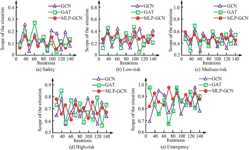
Figure 9 Five security situations test results.
Figures 9(a), 9(b), 9(c), 9(d), and 9(e) represent the numerical tests of security situation assessment of the three models under five NSS scenarios, namely, safety, low-risk, medium-risk, high-risk, and emergency, respectively. Under the five levels of simulated situations, both GCN and GAT models have some assessment results beyond the range of each level of situation. In particular, in the emergency situation, the GCN and GAT models show strong discrete assessment results of 0.64 and 0.71. Although the MLP-GCN model’s assessment results are more volatile in this posture than in the other four, the assessment results also all remain within the posture range of 0.8 to 1.0. In summary, the two models, GCN and GAT, fail to accurately assess the NSS. In contrast, all the assessment results evaluated by the MLP-GCN model proposed in the study are within the range of each level of posture. The fluctuations are smaller than the other two models, and the evaluation results are more stable. Especially in the complex NSS, it can still maintain a high assessment accuracy. This validates the applicability of the model for assessing NSS. The study plots the computation time of each model under five situations. The results are shown in Figure 10.
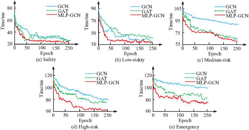
Figure 10 Five security situation assessment time test results.
Figures 10(a), 10(b), 10(c), 10(d), and 10(e) represent the security situation assessment time tests of the three models for five NSS scenarios, namely, secure, low-risk, medium-risk, high-risk, and emergency, respectively. As the security situation level increases, the time required for the initial evaluation of all three models increases accordingly. However, the amount of time needed to finish a situation assessment progressively drops as the number of model training cycles rises. This indicates that the CE of the models can be improved by training the models. The shortest time required for the MLP-GCN model constructed in the study is 22.4 ms, 32.3 ms, 57.8 ms, 61.9 ms, and 74.7 ms for the assessment under the five security situations, respectively. It is significantly better than that of the GCN model, which is 30.6 ms, 41.2 ms, 97.3 ms, 90.6 ms, and 113.5 ms. The difference in the shortest computation time between the MLP-GCN and GAT models is not significant in the three postures from safe to medium risk. However, the shortest computation times of 61.9 ms and 74.7 ms for the models constructed in the study are also better than the 80.7 ms and 83.3 ms for the GAT model in the two states of high risk and emergency. In conclusion, the MLP-GCN model developed for the study has superior CE and can quickly finish evaluating complicated NSS. All the above tests are evaluated under a single static NSS. Therefore, the study continues to construct the dynamic NSS and validate it with the average accuracy, average evaluation time, and resource utilization as the reference metrics. Table 4 displays the validation findings.
Table 4 Index test of different models in different situation
| Average | Average Assessment | Occupancy | ||
| Situation | Model | Accuracy/% | Time/ms | Rate/% |
| Static | GCN | 82.43 | 42.16 | 30.33 |
| GAT | 86.62 | 32.74 | 66.74 | |
| MLP-GCN | 96.54 | 24.36 | 45.25 | |
| Dynamic | GCN | 75.68 | 94.82 | 35.93 |
| GAT | 82.96 | 86.63 | 72.61 | |
| MLP-GCN | 94.59 | 66.19 | 53.87 |
In Table 4, in both static and dynamic scenarios, the average assessment accuracy of the MLP-GCN model is 96.54% and 94.59% respectively. It is almost 10% higher than that of the GAT model and much higher than that of the GCN model (82.43% and 78.96%). In terms of assessment time, the required assessment time of all three models is somewhat prolonged in the dynamic scenario. However, the model constructed in the study still shows obvious advantages. Its average evaluation time in the dynamic scenario is 66.19 ms, which is shorter than 94.82 ms for GCN and 86.63 ms for GAT. In terms of computing resource occupancy, the occupancy of the three models in the dynamic case is also higher than that in the static case. The MLP-GCN model has an occupancy rate of 45.25% and 53.87% in the two scenarios, respectively. Due to the higher complexity of the model itself, the occupancy rate is higher than that of the single GCN model, but lower than that of the GAT model. In summary, the MLP-GCN model constructed in the study also shows superior performance over the rest of the models in the complex dynamic NSS. It is able to maintain higher evaluation accuracy and shorter evaluation time with lower resource utilization. The evaluation model not only needs to perform well on known datasets, but also should possess strong generalization capabilities to cope with the complex and ever-changing network environment in the real world. To evaluate the potential of the MLP-GCN model in this regard, the study conducts a cross-dataset evaluation experiment. The model is trained on the CICIDS dataset and tested directly on the NSL-KDD dataset without fine-tuning. NSL-KDD is a classic benchmark dataset that differs from CICIDS and UNSW-NB15 in terms of feature distribution and attack types. This test can effectively simulate the performance of the model when encountering unknown network threats and topological structures. For comparison, the GCN and GAT models also undergo the same tests. The results are shown in Table 5.
Table 5 Test results of cross-dataset generalization ability
| Training Dataset | CICIDS | CICIDS | CICIDS |
| Test dataset | NSL-KDD | NSL-KDD | NSL-KDD |
| Model | GCN | GAT | MLP-GCN |
| Accuracy (%) | 78.34 | 81.56 | 85.79 |
| F1-score (%) | 76.89 | 80.12 | 84.33 |
| ROC-AUC (%) | 85.21 | 88.45 | 91.67 |
In the results of Table 5, when the comparison models are confronted with NSL-KDD data, the performance of all models decreased as expected, which reflects the domain difference challenges brought about by different network environments. However, the proposed MLP-GCN model still maintained the highest performance level, with an accuracy rate of 85.79% and an ROC-AUC of 91.67%. This is significantly better than the performance of the comparison models. The results show that the MLP-GCN model’s ability to perceive topological structures and its ability to learn deep node feature representations through GCN and MLP, respectively, have high universality and can capture universal network security patterns beyond specific datasets. Compared with the baseline model, MLP-GCN shows stronger adaptability and robustness to changes in data distribution and unknown attack types.
4 Conclusion
Heterogeneous data processing is difficult in NSSA, complex network topology correlation FE is insufficient, and dynamic threat response is inefficient. Therefore, the study innovatively proposed a hybrid assessment model fusing MLP and GCN. The experimental results indicated that when the MLP HL was 3 and the learning update rate was 0.0005, the accuracy of the model reached 96.5% and 94.3% on CICIDS and UNSW-NB15 datasets, respectively. It was significantly higher than traditional models such as GCN, RF, and GAT. In addition, the model showed good performance in metrics such as recall and F1, with an improvement of about 2%–10% over the remaining models. It verified its significant advantages in FE and classification performance. In the simulation test of APT-KGD, the model’s NSSA results for the five grades of safety, low risk, medium risk, high risk, and emergency were between (0.05–0.16), (0.24–0.39), (0.51–0.60), (0.64–0.79), and (0.81–0.99), respectively. These results were limited to the assessment range set for each level. Moreover, the fluctuation range was smaller, the fluctuation range was about within 0.15, and the assessment stability was better than that of the GCN and GAT models. Especially in the emergency situation, the model could still maintain the accurate assessment range, which fully reflected its ability to adapt to the complex network environment. In the dynamic NSS test, the average accuracy of the model was 94.59%, the average evaluation time was 66.19ms, and the resource consumption rate was 53.87%. The model could realize efficient and accurate evaluation with low resource consumption, showing strong practicality and robustness. In summary, the MLP-GCN model proposed in the study solves the limitation problem of existing methods in heterogeneous data processing by combining the node FE capability of GCN and the deep feature learning capability of MLP. However, this study still has some limitations, which point out the direction for future research. The first issue is scalability: The current model encounters computational and memory bottlenecks when dealing with ultra-large-scale network graphs due to the full-graph convolution operation of GCN. Future work will explore hierarchical GCN, subgraph sampling or distributed graph learning techniques to enhance the applicability of models in large-scale networks. Then there is adversarial robustness: The model may be vulnerable to targeted adversarial attacks. Attackers can manipulate the evaluation results by slightly altering the input data or the graph structure. The next key area of research will be enhancing the robustness of models, for instance through adversarial training or by combining graph structure learning with robust optimization. In conclusion, future research will address the aforementioned challenges of scalability, real-time performance, and security by optimizing algorithms and improving architecture. This will promote the application of this model in more complex and dynamic network environments.
References
[1] Khan M, Ghafoor L. Adversarial machine learning in the context of network security: Challenges and solutions. Journal of Computational Intelligence and Robotics, 2024, 4(1): 51–63.
[2] De Keersmaeker F, Cao Y, Ndonda G K, Sadre R. A survey of public IoT datasets for network security research. IEEE Communications Surveys & Tutorials, 2023, 25(3): 1808–1840.
[3] Su J, Jiang M. A hybrid entropy and blockchain approach for network security defense in SDN-based IIoT. Chinese Journal of Electronics, 2023, 32(3): 531–541.
[4] Guo Y, Zhang S. Research on Construction and Application of Network Security Situational Awareness Platform Based on Big Data. IEIE Transactions on Smart Processing & Computing, 2025, 14(2): 218–228.
[5] Cheng M, Li S, Wang Y, Zhou G, Han P, Zhao Y. A New Model for Network Security Situation Assessment of the Industrial Internet. Computers, Materials & Continua, 2023, 75(2): 31–35.
[6] Sun J, Li C, Song Y. A network security situation prediction approach based on MAML and BiGRU. Journal of Intelligent & Fuzzy Systems, 2024, 47(4): 307–319.
[7] Yu Y. A network security situation assessment method based on fusion model. Discover Applied Sciences, 2024, 6(3): 97–98.
[8] Wang Q, Ren X, Li L, Pen H. Design of Network Security Assessment and Prediction Model Based on Improved K-means Clustering and Intelligent Optimization Recurrent Neural Network. International Journal of Advanced Computer Science & Applications, 2024, 15(6): 17–19.
[9] Xu X, Zhao X, Wei M. A comprehensive review of graph convolutional networks: approaches and applications. Electronic Research Archive, 2023, 31(7): 4185–4215.
[10] Yang H, Li Z, Qi Y. Predicting traffic propagation flow in urban road network with multi-graph convolutional network. Complex & Intelligent Systems, 2024, 10(1): 23–35.
[11] Reka R, Karthick R, Ram R S, Singh G. Multi head self-attention gated graph convolutional network based multi-attack intrusion detection in MANET. Computers & Security, 2024, 136: 103–106.
[12] Presekal A, Ştefanov A, Rajkumar V S, Palensky P. Attack graph model for cyber-physical power systems using hybrid deep learning. IEEE Transactions on Smart Grid, 2023, 14(5): 4007–4020.
[13] Alarab I, Prakoonwit S. Graph-based lstm for anti-money laundering: Experimenting temporal graph convolutional network with bitcoin data. Neural Processing Letters, 2023, 55(1): 689–707.
[14] Shi W, Zhang J. Integration of local position-POS awareness and global dense connection for ABSA. Journal of Experimental & Theoretical Artificial Intelligence, 2025, 37(3): 391–411.
[15] He H, Yu X, Zhang J, Song S, B. Letaief K. Message passing meets graph neural networks: A new paradigm for massive MIMO systems. IEEE Transactions on Wireless Communications, 2023, 23(5): 4709–4723.
[16] Pal S, Roy A, Shivakumara P, Pal U. Adapting a Swin Transformer for License Plate Number and Text Detection in Drone Images. Artificial Intelligence and Applications, 2023, 1(3): 145–154.
[17] Raja M W. Artificial Intelligence-Based Healthcare Data Analysis Using Multi-perceptron Neural Network (MPNN) Based On Optimal Feature Selection. SN Computer Science, 2024, 5(8): 1034–1035.
[18] Lu J, Lan J, Huang Y, Song M, Liu X. Anti-attack intrusion detection model based on MPNN and traffic spatiotemporal characteristics. Journal of Grid Computing, 2023, 21(4): 60–65.
[19] Zhang J, Li C, Yin Y, Zhang J, Grzegorzek M. Applications of artificial neural networks in microorganism image analysis: a comprehensive review from conventional multilayer perceptron to popular convolutional neural network and potential visual transformer. Artificial Intelligence Review, 2023, 56(2): 1013–1070.
[20] Altay O, Varol Altay E. A novel hybrid multilayer perceptron neural network with improved grey wolf optimizer. Neural Computing and Applications, 2023, 35(1): 529–556.
[21] Q. Wu, “Network Security Maintenance and Detection Based on Diversified Features and Knowledge Graph”, JCSANDM, vol. 14, no. 02, pp. 339–364, Jun. 2025.
[22] K. Somsuk, “Enhanced Algorithm for Recovering RSA Plaintext when Two Modulus Values Share At least One Common Prime Factor”, JCSANDM, vol. 14, no. 02, pp. 433–456, Jun. 2025.
Biographies

Xiaofeng Zhao, male, born in October 1970, is a senior experimentalist at Anhui University of Finance and Economics. He holds a Master of Engineering degree from the University of Science and Technology of China. His main research directions are information security and network management. In recent years, he has mainly taught courses such as Computer Network and Computer Network Security. Over the years, he has published more than ten papers as the first author in EI and CSCD journals, participated in the completion of multiple horizontal projects, co-authored three computer professional textbooks, and authored a monograph on network security.

Qianjun Wu, a senior engineer majoring in Computer Science and Technology. Since June 2007, I have been working at Bengbu City Pass Card Co., LTD., successively holding positions such as Deputy director and director of the Technology Management Center, Deputy general manager and general manager of the company, responsible for accounting Planning, design, construction, implementation and operation of related work such as computer software and hardware development, information construction and intelligent engineering. Led the development and construction of: Bengbu City One-Card Project (including the construction of the clearing center), Bengbu Public Transport Informationization (including ERP, computer room construction, etc.) projects, the interconnection project of the Ministry of Transport’s transportation one-card, and the “Internet” of Bengbu City Pass “Recharge platform system project, etc.”

Peng Wang, obtained a Bachelor’s degree in Electronic Engineering from Anhui University in July 1999 and a Master’s degree in Electronic and Communication Engineering from Nanjing University of Science and Technology in January 2008; In May 2011, he was selected as one of the “Six One Batch” Double Hundred Talents in the Anhui Provincial Propaganda and Culture System. At present, he serves as the deputy director and senior engineer at the Bengbu Network Security Emergency Center, mainly engaged in network security, data security and other work. He has independently published 9 papers in national level journals.
Journal of Cyber Security and Mobility, Vol. 15_1, 1–24
doi: 10.13052/jcsm2245-1439.1511
© 2026 River Publishers