Throughput Prediction Across Heterogeneous Boundaries in Wireless Communications

Received 21 January 2016; Accepted 30 January 2016;
Publication October 2015

Rayyan Sayeed¹, Raymond Miller² and Zulfiquar Sayeed²

• ¹Drew University, Madison, NJ, USA
• ²Bell Laboratories, 600 Mountain Avenue, Murray Hill, NJ, USA

Email: rsayeed@drew.edu; {ray.miller; zulfiquar.sayeed}@nokia.com

---

Abstract

In this paper we demonstrate how an estimated functional kernel-regression polynomial from a particular RF technology can be created by the mobiles being served by that technology. A 3rd order polynomial description of the regression can be used to predict future throughput by observing the “pilot” quality prior to handover. The UE may use it to predict the throughput it will get in the new technology 50 to 200 m-sec prior to handover. The prediction can inform the Transport Control Protocol (TCP) layer or the application layer of the upcoming handover and the throughput expected after handover so that the user application receives the best quality of service. This paper is an extended version of the paper presented at IEEE Sarnoff Symposium 2015 [1]. It extends the paper with expanded foundational knowledge and explanation of the results and their implications.

In this paper we:

• propose that there is a way to predict the unobservable quality metrics in the new cell prior to commencement of the handover. This is achieved by1) a prediction mechanism and 2) a signaling mechanism. In this paper we focus on the prediction mechanism.
• propose that the observable metric (“pilot” quality) is predicted with prediction error below 9% with prediction step sizes of 200 m-sec.
• show that the throughput metric (we choose bits/physical-resource-block = β) can be predicted with error below 8% with prediction horizon of 200 m-sec.

---

Keywords

• Data Analytics
• LMS
• Functional Regression
• Prediction
• 5G
• LTE
• Handover

1 Introduction

In wireless communications, handover occurs when one cell signal diminishes in link quality, and another cell’s signal increases in link quality. This change in link quality occurs commonly when the mobile device or User Equipment (UE) is moving. There are many factors that affect the strength of a signal as it transits from a broadcasting antenna to a receiver. These factors are path loss, slow fading, fast fading, and noise [2].

Path loss refers to the gradual loss of signal power that occurs during travel from a broadcast source to a receiver. Power diminishes exponentially due to path loss, with the exponent depending on environmental factors. The HATA model [2] (named after M. Hatay) is an empirical model for path loss that will be used to simulate path loss. Slow fading occurs when a signal is obstructed during its path to the receiver, i.e. by buildings or other objects. Slow fading is log-normal. Fast fading, or multipath fading, occurs when a signal is reflected by multiple objects in its path to the receiver. This results in the signal arriving at the receiver from multiple paths, and with a uniform angle distribution. Fast fading follows a Rayleigh distribution, and the received signal power is correlated with space.

The interaction of these perturbation factors upon the signal of interest in telecommunications complicates the point of handover. Quite often, it is increasingly difficult for a mobile device to switch signal sources without an interruption of service to the user [3]. This interruption occurs because the application server (for example a YouTube server) and/or the Transport Control Protocol (TCP) stack [4] have no knowledge of the LTE (Long Term Evolution) network state. This network state determines how much throughput, or bandwidth, is available to the mobile device. It is calculated, in[4], that the TCP New Reno protocol stack has a 40% chance of overflowing its buffer if the handover latency is about 50 m-sec. In [5], it has been reported that in Frequency Division Duplex (FDD) LTE, which is what we study here, the connected mode latency for handover is about 22 m-sec. But, the TCP stack reacts to the user data disruption time, which as we shall see in Section 3, is 70 m-sec. Therefore, at this disruption duration the TCP protocol stack with 40+% likelihood will overflow. Disruption at the TCP layer leads to severe application layer rate loss, spurious re-transmissions, duplicate ACK (ACKnowlegement) reception, slow-start [6]. These are disruptive to the application the subscriber is using on the UE at the time of handover.

The process of handover in LTE is detailed in [3]. There are several time periods involved in handover.As noted in the reference – “Previous works have shown that it is not a trivial task to set appropriately HO hysteresis and TTT, since the optimal setting depends on UE speed, radio network deployment, propagation conditions, and the system load”

• Time to Trigger (TTT): is the period of time during which the neighbor RSRQ should be stronger than the serving cell. A nominal value could be 50 to 100 m-sec (vendor specific).
• A4 (Neighbor becomes better than threshold) delay: 10 to 100 m-sec (vendor specific).
• UE measurement Delay: The time UE measures Reference Signal Received Quality (RSRQ) to report to eNodeB. Nominally may be 100 to 500 m-sec (vendor specific).
• UE measurement period: 100 to 500 m-sec(vendor specific).

Note that the UE is capable of observing the “pilot” signal quality of neighbor cell much before actual data disruption occurs in the handover process. Hence our prediction time is not set by the handover duration of 22 m-sec cited in [5], but the actual time that the UE can receive the neighbor cell prior to handover which is in the tune of perhaps more than a second from the list above. Eventually the duration of prediction is a function of cell layout, UE velocity, RF conditions etc. We feel confident that, with the above listed delays, The UE shall have ample time to predict the neighbor cell’s future RSRQ.

In order for user service and for TCP to be uninterrupted after handover occurs, we can create a prediction of the throughput that would be achievable after the handover - before we make the handover. This information, with new signaling techniques (not discussed in this paper) can be used by the TCP or the application server to find the optimum bandwidth expectation before the handover takes place. Handover prediction has been reported for LTE in [7] based on the UE position history and in [8] for Wi-Fi using the IEEE Standard 802.21 (Media Independent Handover). In [8], handover event is predicted based on serving cell RSSI (Received Signal Strength Indicator). Once the handover is predicted [8] uses 802.21 protocol to instruct the required time for handover to the candidate cell. It does not offer a means of telling the TCP layer or the application server the throughput to be expected after the handover is complete. The latter step must be done with the candidate cell “pilot” quality which we do in this paper.

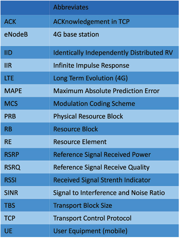
Figure 1 List of acronyms used in this paper.

The channel quality metrics of Signal to Interference Ratio (SINR), Receive Signal Strength Indicator (RSSI), and Reference Signal Received Quality (RSRQ) are useful in handover decisions, and the mapping of metrics such as these to the UE’s received throughput is functionally dependent on the eNodeB (Enhance Node B – base station in LTE) algorithms and the RF-frontend characteristics.

In this paper, we predict the future throughput as, β, the bits per Physical Resource Block (PRB) (we call this β) from the past throughput. We use the RSRQ metric to base our predictions. RSRQ is defined as follows:

$$\begin{array}{rr}\hfill RSRQ=N\times \frac{RSRP}{RSSI},& \hfill (1)\end{array}$$

where, RSSI is the Received Signal Strength Indicator and is the signal power received over the entire LTE band (in our case the 5 MHz wide LTE carrier), and N is the number of physical resource blocks in the LTE carrier (for 5 MHz carrier N = 25), and RSRP (Reference Signal Received Power) is power received in the Reference signal part of the LTE carrier. In the LTE carrier, there is 1 Resource Element (RE)¹ dedicated as a “pilot” or reference signal and is transmitted once every 6 REs. The placing of the RE is a function of a cell-ID which enables the UE to measure signals for its attached eNodeB and the neighbor eNodeBs simultaneously, albeit with interference from each signal [9].

The rest of the paper is organized as follows. In Section 2, we describe the methodology used in our prediction. In Section 3, we describe the wireless network simulation and the parameters used. Section 4 explores our results. The paper concludes with our summary and planned next steps in Section 5.

2 Methodology

We first estimate the future RSRQ by measuring it for both the current eNodeB and the future possible eNodeBs with which the UE will connect. Then a mapping is made from the RSRQ to the β from past observations by the UE by using non-parametric functional regression techniques [10]. Once the functional regression is complete, the predicted RSRQ of the candidate eNodeB is used to predict the β in the candidate cell in the future. In the same method, the application could anticipate the throughput (a function of SE) the mobile may have after the handover has been made, and must match what the mobile may receive. The problem here lies in the fact that, under current conditions, the application server/TCP Sender and the application client/TCP Receiver on the mobile-end have no way of communicating with the radio layer where the actual capacity/throughput is measured. The goal of this paper is to use a simulation to recreate these mobile conditions, and then analyze the data using statistical tools. This analysis should give us a way of predicting the new link quality and throughput of the new eNodeB before handover occurs, so that the application server or TCP stack will be able to adjust throughput expectations for proper application/TCP behavior.

As a background [9] on LTE transmission and reception, the metrics of interest are calculated in the following manner:

1. The UE receives the downlink transmission from the eNodeB.
2. The UE calculates the SINR of the received signal by way of embedded pilot tones in the received signal.
3. The UE calculates the Channel Quality Indicator (CQI) based on capacity calculations (for example for AWGN channels) and feeds back the CQI to the eNodeB [11].
4. The eNodeB receives the CQI and forms its understanding of the SINR of the UE.
5. The SINR calculated in 4 is used to select the Modulation Coding Scheme (MCS) for the UE in the next TTI. Thus, MCS is a channel quality driven metric. The UE signal processing capabilities also play a role in the MCS selection.
6. The eNodeB obtains the number of Physical Resource Blocks (PRBs) to be allocated to the UE in the next Transmission Time Index (TTI) by using the cell load and its scheduler algorithm. The PRB count is strictly driven by load and Quality of Service (QoS) assignment for that UE (actually its bearer). One PRB is made of 84 (12 × 7) resource elements.
7. The MCS and PRB, calculated in (5) and (6) above, are used to calculate the Transport Block Size (TBS), in number of bits, for transmission in the next TTI by way of the lookup table of 3GPP standard document TS36.213. Thus, the TBS embodies the effects of the channel, load and the algorithmic behavior of the communication chain.8. The UE continually measures the serving cell RSRQ or RSRP while in connected mode from the eNodeB it is connected to
8. The UE measures the RSRQ or RSRP of neighbor cells periodically for handover purposes [3, 12]. In our work, we assume that RSRQ measurements in the candidate cell is available at least 10 m-sec prior to handover, every TTI (Transmission Time Interval=1 m-sec).
9. We create an additional metric from the available outputs from the UE:

   i. β. β is defined as

   $$\begin{array}{rr}\hfill \beta \left(i\right)=\{\begin{array}{ll}\frac{tbs(i)}{prb(i)}\hfill & \text{if}prb\left(i\right)\ne 0\hfill \\ 0\hfill & \text{otherwise}\hfill \end{array}& \hfill \left(2\right)\end{array}$$

   where, i indexes the TTI sequence.

The significance of β is that it represents the number of bits that could have been sent had the scheduler allocated a PRB to the user of interest. The definition of β ensures that:

• Only those bits that are actually received by the UE are taken into account. LTE operates in the design range of 1 to 10% packet error rate. β only includes the error-free received bits. The TBS metric reported from the eNodeB ensures that only error-free bits are reported.
• The role of the scheduler is totally taken out of the metric as we only use granted intervals to calculate β and then interpolate the missing TTI values. This is ensured by the condition that prb(i) ≠ 0. In fact, PRB is reported as 0 for re-transmissions, and when the UE is not scheduled, the metric is missing in the log files.

Note that the modeling, function learning, and prediction of higher level metric such as the throughput (β) will not only try to capture the behavior of nature (as in SINR modeling) but also capture the evolution and dependencies that exist in possibly intractable eNodeB and UE algorithms, user behavior, other user behavior, and the entire network as a whole. This is achieved by linear polynomial regression on the RSRQs, followed by a non-parametric functional learning of RSRQ to β, and then the eventual prediction of β from the predicted RSRQ.

As described above, we use the metrics available from the UE in unconnected mode, namely the RSRQ, a quality metric as opposed to an absolute metric of RSSI, as shown in Equation 1, to predict the future value of that metric. We then use functional techniques to learn the “dependent” metric’s relationship to RSRQ from past observations at the UE. This past observation interval is called the training interval. Such training is envisioned to have happened in heterogeneous wireless connections so that a functional map can be established from RSRQ (in case of LTE) or RSRQ-like metrics (in other 5G air interfaces).

The metric of interest is β in LTE and β-like in other air interfaces. The philosophy is that as β represents the number of bits that the receiver can get in the most fundamental transmission unit (1 PRB) in LTE, a similar metric must be created in the neighboring heterogeneous cell. The portability of the β metric is desirable as it is devoid of the scheduler impact. From the structure of resources in a radio network, the application layer or the TCP stack can calculate the minimum throughput the UE may expect after handover had the UE been granted the minimum resources.

Thus, we predict an observable variable, functionally map it to past observed values of the desired metric, and predict the unobservable metric in the new cell by way of observing and predicting the observable metric of the new cell prior to handover. The decision to handover to the new cell will be UE-centric (or maybe rather user-centric) in the future [13], and such forecasting capability would enable the UE to make better decisions given the application demands, and/or the user’s preferences or profile.

In our paper we use LTE as the present and future network. However, we train the RSRQ on the received metrics from the two base stations prior to handover and then estimate the new base-station’s possible throughput by using the RSRQ from the new base station. The functional mapping is learned from the current base-station, and because of homogeneity, can be used in the next network. We envision that a functional map (which could a vector of a hundred samples long) can be either learned by the UE in its sojourn at the heterogeneous technology in the past or the neighbor cell’s functional map can be stored in or transmitted to the UE by the current serving base-station. That is for further study. Here we establish the feasibility of the statistical processing. In our case, we use the same functional regression learned from one velocity for other velocities in our simulation. For function learning, what is necessary is statistical richness of the values of the observation and not simply the time required to train.

In Figure 2, the flow of the steps for RSRQ predicted β prediction is shown. The UE produces internal metrics as described in Section 1. For every TTI (1 m-sec), we collect the metric corresponding to β and RSRQ. We apply a smoothing function (in our case an averaging every τ samples which we vary in our simulation between 50 to 200 m-sec for β and 10 to 100 m-sec for RSRQ) to smooth out fast variations and to see the effects of channel-memory and noise smoothing on the prediction performance.

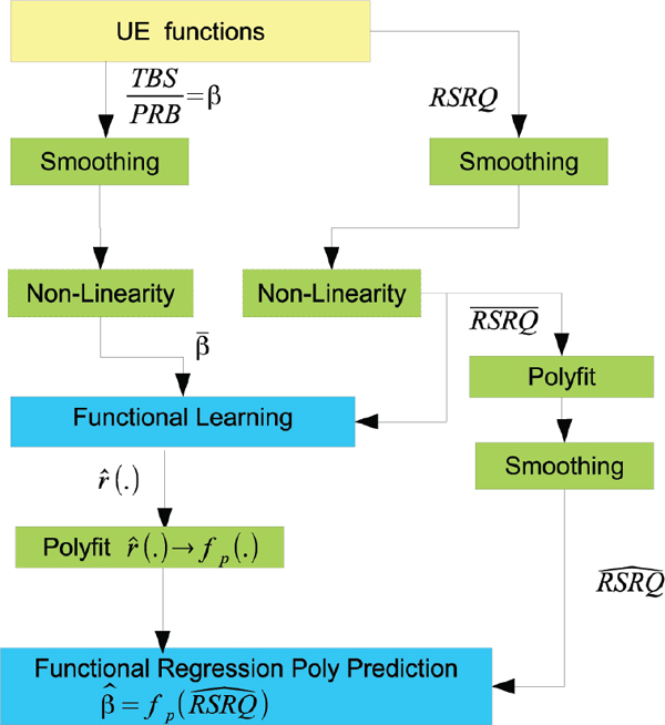
Figure 2 Flow of information for functional prediction of β.

Some TTI metrics may be zero, due to eNodeB scheduler algorithm, in which case we use an interpolator to fill in missing data, and then smooth. We introduce (optionally) a non-linearity, which is 10log() in our case, in line with producing homoscedasticity, that is, to try to make variances homogeneous across metrics of interest (in time), if needed, as described in [14]. [14] uses a log non-linearity to produce homoscedasticity for heteroscedastic SINR RMS(Root Mean Square) value prediction for IEEE 802.16. The non-linearity is not for smoothing purposes.

The smoothed RSRQ and β are then sent to the functional learning block. This is based on the non-parametric functional regression technique of [10]. We find the functional relationship between RSRQ = X to β = y. The input and output is related by the relationship:

$$\begin{array}{rr}\hfill y_i=r\left(X_i\right)+{\epsilon }_i& \hfill \left(3\right)\end{array}$$

where, ɛ_i is the error term and r() is estimated by:

$$\begin{array}{rr}\hfill \widehat{r}\left(X\right)=\frac{{\displaystyle {\sum }_{i=1}^{n}K\left(h^{-1}d\left(X,X_i\right)\right)y_i}}{{\displaystyle {\sum }_{i=1}^{n}K\left(h^{-1}d\left(X,X_i\right)\right)}}& \hfill \left(4\right)\end{array}$$

where his the smoothing parameter (evaluated by the method of [16]) and dis a distance-metric (in our case it is simply the Euclidean distance $d\left(x_1,x_2\right)=\sqrt{{\left(x_1-x_2\right)}^2}$ and we select the kernel K to be the Triweight kernel:

$$\begin{array}{rr}\hfill K\left(u\right)=\frac{35}{32}{\left(1-u^2\right)}^{2}1\left\{\left|u\right|\le 1\right\}.& \hfill \left(5\right)\end{array}$$

We have evaluated with a variety of kernels and Triweight yields the best performance for our purpose. The $\widehat{r}\left(X\right)$ function is then fitted into a polynomial f_p(X) for ease of signaling and reduction of calculation complexity. We use the predicted $RSRQ=\widehat{RSRQ}$ to evaluate the predicted β value by way of the function f_p(X). We have tried several polynomial orders for f_p(X) and order 3 has been found to be sufficient given the general shape of $\widehat{r}\left(X\right)$.

3 Simulation Setup

In Figure 3, we show two trajectories of the UE during handover. The horizontal one is our primary focus in this paper. The blue, slanted one is discussed at the end of Section 4.

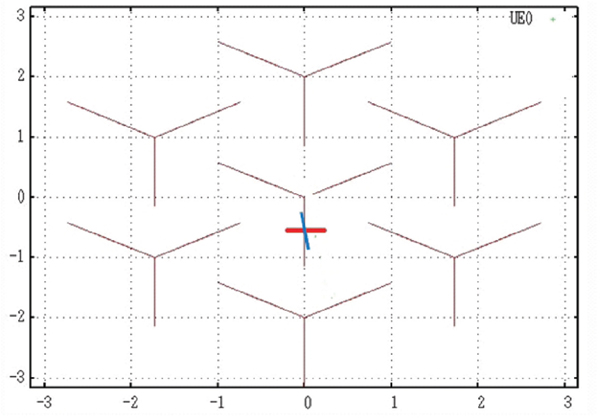
Figure 3 Handover Trajectories (axes in KMs). The 7 eNodeBs are located at the heart of the “Y”s, and each 120 degree is served by a sector antenna. The 7 “Y”s represent a canonical 7-cell Hexagonal layout.

In our simulation we generate the eNodeB metrics by using a proprietary Alcatel-Lucent sample level simulator. The salient settings of the simulator for this paper are as below:

• Carrier Frequency (DL): 700 MHz
• Carrier: FDD, 5 MHz (25 PRBs)
• Number of cells: Hexagonal 7 (3 sectors per cell)
• Cell Radius: 1 KM
• UE velocity: 3, 10, 30 km/hr
• UE local clutter velocity: 3, 10, 30 km/hr
• UE of interest traffic: Constant Bit Rate (CBR), 6 MBPS
• UE Receive mode: 2 Rx Antennas, Antenna Selection Off
• CQI reporting: periodic every 20 m-sec
• Rayleigh Channel Model for 3 km/hr (ITU Pedestrian A Model):

  Relative Delay (ns)	Relative Power (dB)
  0	0.0
  110	–9.7
  190	–19.2
  410	–22.8

• Rayleigh Channel Model for 10 km/hr (ITU Pedestrian B Model):

  Relative Delay (ns)	Relative Power (dB)
  0	0.0
  200	–0.9
  800	–4.9
  1200	–8.0
  2300	–7.8
  3700	–23.9

• Rayleigh Channel Model for 30 km/hr (ITU Vehicular A Model):

  Relative Delay (ns)	Relative Power (dB)
  0	0.0
  310	–1.0
  710	–9.0
  1090	–10.0
  1730	–15.0
  2510	–20.0

• Other Cell Load: 100
• Simulation Duration: 350 Seconds (750 for 3 km/hr)

The output metrics RSRQ, SINR, TBS, MCS and PRB are saved once every TTI at the eNodeB and UE (RSRQ). For SINR, since CQI reporting is periodic, with 20 m-sec period, the same value is output to the log file between CQI updates. The other metrics change according to the error control loop, scheduler and other algorithms in place at the eNodeB every TTI. If the UE is not to be scheduled in a TTI, then the corresponding PRB and TBS will be zero. If the frame is received incorrectly, then for the subsequent retransmissions of that frame the TBS value is zero, while PRB is non-zero. In the smoothing block of Figure 2, we take such zero possibilities into account and interpolate the values so that the averaging is meaningful given the averaging window size τ . It is important to note that the fading velocities of 3, 10 and 30 km/hr at the carrier frequency of 700 MHz yields Doppler frequencies Δf of 2.1,6.5 and 20.8 Hz, yielding a coherence time [2] of the channel (1/Δf) of 480, 154 and 48 m-sec respectively. In our analysis, we have imposed an additional finite impulse response (FIR) filter on the output of the RSRQ such that the time-span of this filter varies with the coherence time. This can be accomplished by the velocity estimation inherent in UE base-band algorithms or by aid of GPS.

The traces for 30 km/hr are shown in Figure 4. The UE periodically traverses the path end-to-end in the 350 second simulation. When it reaches the end of the path, it turns around and travels in the other direction. Handovers occur near the vertical line of the sector separator in Figure 3. These handover points are shown by the [circleasterisk] along the 30 dB line of Figure 4. Note that the RSRQ (magenta curve) is a very noisy signal compared with the traces above it, because the eNodeB filters its metrics. RSRQ is unfiltered. Also, note that the eNodeB metrics saturate when the UE sees the high quality signal to the eNodeB. This occurs about 20 seconds before and after every handover. Since such clipping is non-linear (the eNodeB does clip the SINR from which other metrics are derived at the eNodeB), it does not lend itself well to the linear techniques we are using in this analysis. Therefore, we try to use only the linear parts of the traces, since it is the best way to train the functional regression. This also puts a constraint on the functional regression training signals for the UE. If the regression function is transmitted to the UE, then the onus of such training is at the cell-tower. If the cell-tower is responsible for the functional regression calculation, then the UE should periodically report back the RSRQ to the eNodeB, which would require the signaling to be standardized. We also note that all metrics reach their minima at the time of handover. Thus, this is a difficult problem as we are dealing with traces of low signal to noise ratio, and with UEs moving, creating a mean and variance fluctuations along the paths. The problem is certainly non-stationary. We are thus faced with non-linearities, non-stationarity and low signal power. We have used the poly-fit function over finite durations of 10 to 100 m-secs, where the process may be considered somewhat stationary. However, still variations of the central moments in the signal remain and we use the non-linearity of [14] to ensure we get a good prediction performance.

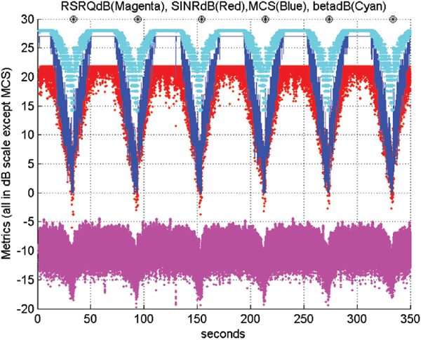
Figure 4 Time series metrics for 30 km/hr traversal.

For lower velocities, we see fewer handovers. The 3 km/hr case hands off only once in the 750 seconds of simulation. For the 3 km/hr case (shown in Figure 5), we use the learned functional regression of the 30 km/hr case, as the latter simulation output is statistically richer. We shall see that prediction still works in such cases, even when the functional learning was done for a different velocity. The functional regression training takes time out of the equation, as can be seen from Equation 4. This is a crucial observation, as the subsequent prediction from observed RSRQ from the new base-station can be done with time only involved with RSRQ evolution, and not the β evolution, as that is absent during handover. In fact, we shall see that the eNodeB’s decision of using a particular rate after handover lags, due to the previously mentioned IIR smoothing in the eNodeB, whereas the RSRQ correctly estimates the β without the lag.

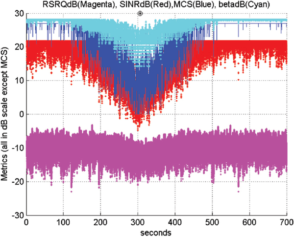
Figure 5 Time series metrics for 3 km/hr traversal (Black circle represents handover point). Note the longer simulation length to obtain a full cycle.

Once the simulated metrics are available after the simulation, we feed the metrics into our algorithms of Figure 2 to do the prediction/regression analysis. We present our findings in the next section.

4 Simulation and Analysis Results

In our analysis, we use Mean Absolute Prediction Error (MAPE) in percentage to evaluate the performance.

$$\begin{array}{rr}\hfill MAPE=\frac{{\displaystyle {\sum }_{i=1}^{N}abs}\left(\frac{A_i-P_i}{A_i}\right)}{N}\times 100& \hfill \left(6\right)\end{array}$$

where A = 10log10 (actual metric),P = 10log10 (predicted metric) and N is the number of samples predicted.

4.1 RSRQ Prediction Performance

As noted in Section 2, we use a non-linearity after the smoothing operation of the RSRQ. In our case, with motion, the metrics are highly heteroscedastic, that is, the independent variable’s (RSRQ) variance is not similar in temporal behavior as that of the dependent variable’s (β), and changes as time varies. We test the prediction performance both with and without the non-linearity. The resultant smoothed RSRQ, after the non-linearity, is introduced into the poly fit() function [15]. This is a very simple predictor where the data is temporally fitted into a polynomial with unknown coefficients with degree N. We use N = 1 because the prediction error decreases with the polynomial order (see Figure 6). The poly-fit is done over 10 smoothed samples.

We have tested the prediction performance by varying the number of samples fitted, and even though the 30 sample duration yields slightly worse performance for RSRQ prediction (see Figure 7, it yields better prediction for the eventual β prediction.

The performance of the RSRQ MAPE for logarithmic and linear training is shown in Figure 8. We notice that smoothing reduces the error. However, we see a counter-intuitive result, that the faster the velocity, the better the performance! This has to do with the channel models used in the simulation as described in Section 3 as ITU pedestrian A, pedestrian B and vehicular A models. These are standard models as described in [17]. These models are used in assessing the performance, and standardized models allow algorithms to be tested in a way that allows comparison across scientific communities.

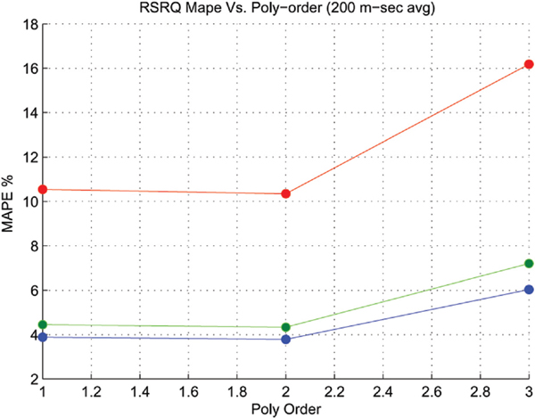
Figure 6 RSRQ prediction error vs. Poly Order At (red: 3 km/hr, green: 10 km/hr, blue: 30 km/hr) Velocities, 200m-sec Averaging, Window of Poly-fit is 10 averaged samples).

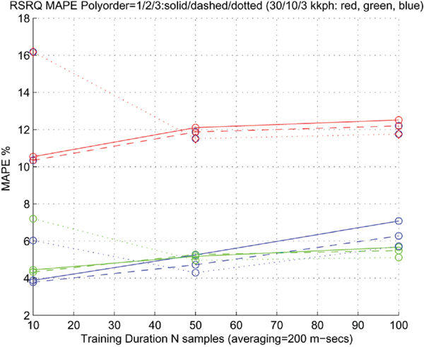
Figure 7 RSRQ prediction error vs. Poly Training Duration. 200 m-sec Averaging. (red: 3 km/hr, green: 10 km/hr, blue: 30 km/hr).

For RSRQ prediction, the correlation between samples is important (slow velocities yield higher correlation of channel metrics) as the poly-fit performs better with correlated data. But the energy of received samples is important as well. The energy indicates how well the LMS can draw a curve through the noisy points. Less energy will mean noise has a bigger role in the degradation of performance. Now (capital letters denote dB),

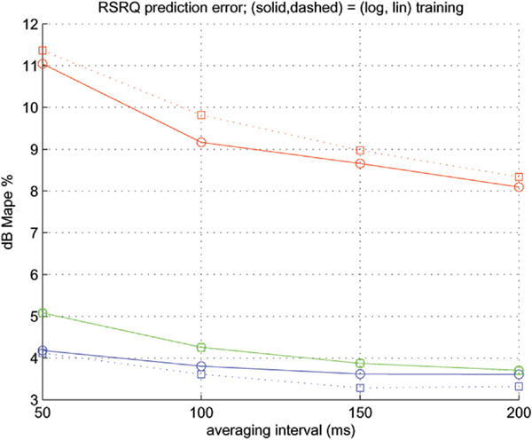
Figure 8 RSRQ MAPE for Log/Lin Poly-fitting (red: 3 km/hr, green: 10 km/hr, blue: 30 km/hr). This represents the MAPE that we can expect at a prediction distance of 50, 100, 150 and 200 m-sec into the future.

$$\begin{array}{rr}\hfill \sin r=\frac{s}{i+n};& \hfill \left(7\right)\end{array}$$

where, s is the signal power, i the interference and n the noise power. During the point of handover, s is almost the same as i. In the dB scale the following can be written

$$\begin{array}{cc}SINR=10{\log }_{10}\left(\frac{s}{i+n}\right)& \left(8\right)\\ ==10{\log }_{10}\left(s\right)-10{\log }_{10}\left(i+n\right)& \left(9\right)\\ ==S-I-10\log 10\left(1+n/i\right)& \left(10\right)\\ \approx S-I-10\left(n/i\right)\ln \left(10\right)& \left(11\right)\end{array}$$

Where, ln (1 + x) = x + ((x²)/2) + ((x³)/3) + … for |x| ≤ 1 (Taylor series expansion) is used in Equation 11, and we keep only the first term as i n; Therefore, SINR ≈ S − I − (4.34 n/i).

In all cases, at handover, s/i ≈ 1; s behaves like i as far as the channel models (losses) are concerned. n is the same for all velocities and i₃≪i₃₀<i₁₀ (subscripts denote km/hr); i₁₀ and i₃₀ are almost the same (from the channel model power profiles in Section 3). Therefore, SINR is smaller for 3 km/hr then the other two velocities.

A velocity of 30 km/hr does perform better than 10 for low averaging – but as we average more the two performances converge as you see in Figure 7. We need to understand why the 30 km/hr case yields better results than the 10 km/hr case. In both cases, we test the algorithm over a set duration length, namely about 40 seconds. The 30 km/hr trajectory recovers from low S − I values faster than the 10 km/hr case. That 40 seconds span the handover region, by design, as that is where we focus to predict the future cell’s β. Hence, temporally, the faster velocity (30) has a better S − I for the duration of the test sequence.

We use the logarithmic non-linearity in our algorithm for the β analysis below as we have observed that the non-linearity yields better predictions for RSRQ.

4.2 β Prediction Performance

On the β path, as shown in Figure 2, we have the same non-linearity as in the RSRQ path after the smoothing block. It should be noted that the UE uses an IIR (infinite impulse response) smoothing filter as below:

$$\begin{array}{rr}\hfill out\left(n\right)=f\ast in\left(n\right)+\left(1-f\right)\ast out\left(n-1\right)& \hfill \left(12\right)\end{array}$$

where f is a positive value less than 1. However, this produces a delay in the path of the β metric which is not there on the RSRQ path. Thus, the two metrics are not aligned appropriately. We alleviate this by applying an IIR filter with f = 0.05 on the RSRQ smoothed output prior to the non-linearity. This may seem to be an inherent divorce from the concept of present channel condition on the eNodeB’s decision on the MCS, TBS; but we are bound by that condition because the eNodeB produces its metrics. Subsequently, IIR filtering RSRQ imposes a penalty on the RSRQ prediction error, but improves the β prediction performance.

The regression function is trained on the past observed RSRQ and β. Ideally, we would train the functional regression with all possibilities of β for a particular RF technology. However, this can be performed by the UE’s past sojourn in that particular RF technology. With RSRQ feedback from the UE to the base-station of a heterogeneous technology, the base-station may formulate the regression function and have it available for the subscribers’ UEs. In our analysis, the training of the functional regression is based on the UE’s sojourn in the 30 km/hr case, which is depicted by the red circles (for the RSRQ) and the parallel β values above, as shown in Figure 9.

The polynomial fit curve of ˆr (RSRQ) (relating β to RSRQ), devoid of time sense, is shown in Figure 10.

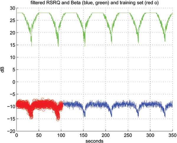
Figure 9 Training β from RSRQs (30 kph)

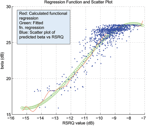
Figure 10 Regression Function (red), poly-fit (green), predicted β (blue) (at 30 kph).

We say “devoid of time sense” because the training involves observation of the independent and dependent variable over a training interval. A matrix is formed with column 1 equal to RSRQ and column 2 equal to β. The matrix is filled temporally. The matrix is ordered in ascending order of the RSRQ value. Then, the two columns are fed into Equation 4. Thus, β prediction is not performed in time, but in functional space.

In a sample prediction run of β, we plotted the test vector against the poly nomial derived from the regression function. The result against the poly-fit is shown in Figure 10 for 30 km/hr with 100 m-sec averaging. The predicted βs are shown as blue dots. The red curve is the regression function, and the green is the polynomial. We use the polynomial to retrieve the prediction because the regression function only has support on the values of RSRQ that were used in training. One difficulty, as mentioned before, is that the training set may include saturated values of actual β. Saturation is a non linear process and does not lend itself to linear techniques. The effect of the saturation shown with the flat dotted surface around –11 to –9 dB RSRQ range. It is expected that by using test vectors with no saturation, prediction would achieve better results.

The prediction of β from predicted RSRQ for 30 km/hr using functional regression is shown in Figure 11. The MAPE of RSRQ and β are 3.92 and5.14% respectively. This prediction occurs over the 2nd handover period of Figure 4. The jump in β is well-predicted by the algorithm; notice the green line and the red dot just to the left of the 94 sec mark.

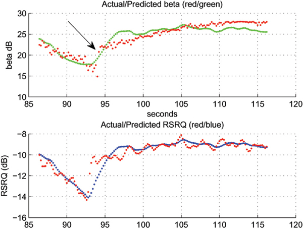
Figure 11 Prediction of β from predicted RSRQ (30 kph, 200 m-sec avg.)

The β prediction MAPE against the averaging duration is shown in Figure 12. It also shows the difference in filtering β prediction with past actual βs. The difference is minor in the time period of the handoff, but we have seen differences in the two performances during the time the UE is in steady-state, that is, when the UE is strongly served by its cell.

4.3 Change in UE Trajectory

For completeness, we also examined a case where the user’s trajectory during handover is not perpendicular to the sector boundary. We chose a new trajectory almost perpendicular to the previous trajectory, that is, the UE traverses the sector demarcation line, except with a slight slant so that handover does occur. Exact sector line traversal does not cause handovers due to handover algorithm hysteresis [3]. The trajectory is shown as the blue slanted line in Figure 3. The traces for this simulation are shown in Figure 13 for UE velocity of 30 km/hr.

We trained the functional regression only once with the horizontal trajectory and used that function to predict both the horizontal and slanted trajectories during the second handover event. The result is shown in Figure 14.

The results of the error rates are about the same in both cases – with the slanted trajectory showing less errors in both β and RSRQ prediction than the horizontal case.

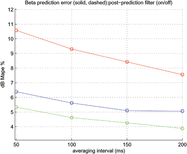
Figure 12 Beta prediction error vs. Averaging Duration (m-sec); RSRQ Poly-fit order 1; red: 3 km/hr, green: 10 km/hr, blue: 30 km/hr.

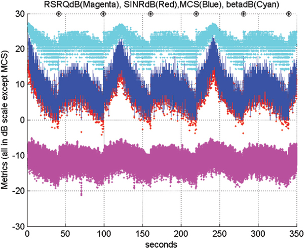
Figure 13 Traces of the Slanted Trajectory at 30 km/hr. Notice the asymmetry of the traces between the handovers due to the trajectory change.

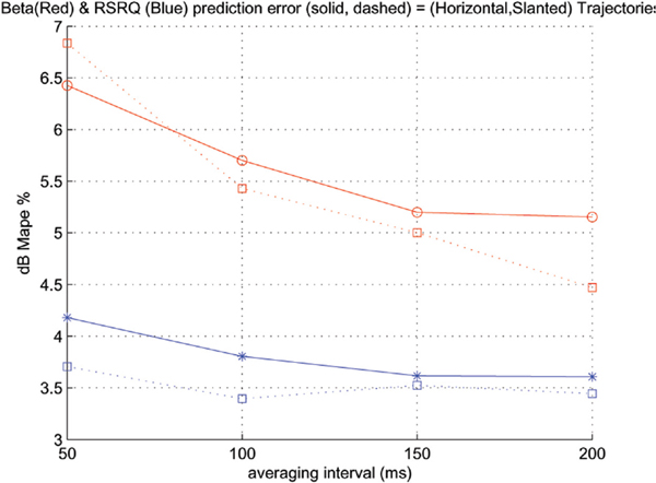
Figure 14 Prediction errors vs. Averaging Duration of the two trajectories (30 km/hr).

5 Conclusion and Further Work

In this paper, we have shown how a functional regression map from a particu lar RF technology can be created by the UEs being served by that technology. This regression function need not be large; a 100 sample vector would suffice. Even the coefficients of a polynomial of order 3 (4 real numbers) may suffice. The heterogeneous technologies can transmit the regression function to the UE, so that it may use it to predict the throughput it will get in the new technology. This prediction can occur 100 m-sec prior to handover by the UE observing less than 10 samples of the new technology’s pilot (RSRQ) quality (Figure 7). This enables the UE or the network (if signaling is established from UE to base-station) to inform the TCP layer or the application layer of the upcoming handover and the throughput expected after handover. Given the durations listed in Section 1 (TTI, A4, etc), this is plenty of time to predict the future value of RSRQ and map that into the expected β in the new cell.

This prediction mechanism needs to be in place in the 5G networks so that the user experience, the TCP layer adjustments and the application layer rate can be optimized across heterogeneous technology boundaries.

For further work, we would like to itemize the following:

• Create the signaling protocols and messaging that enables the UE’s forecasting capability.
• Devise a way to deal with metric saturation in training of the functional regression.
• Analyze the error floor observed in the β prediction error for 10 km/hr.
• Explore Recursive Least Squares methods (Kalman filters) for RSRQ prediction.
• Look at high velocities – up to 200 km/hr for trains. Thus far, we have seen errors decrease with velocity, but that is primarily a power-delay-profile phenomenon.

Ackowledgements

This work was made possible by the Research Institute of Scientists Emeritus (RISE) program of Drew University, Dr. Louis Hamilton of the Drew University Baldwin Honors program, and Drs. Todd Sizer and Sameer Sharma of Bell Labs.

References

[1] Sayeed, R., Miller, R., and Sayeed Z. (2015). “Forecasting of throughput across heterogeneous boundaries in wireless communications: algorithm and performance,” in The 36th IEEE Sarnoff Symposium, Newark, NJ, USA, 1–6.

[2] Sklar, B., et al. (1997). Rayleigh fading channels in mobile digital communication systems part I: characterization. IEEE Commun. Mag. 35, 90–100.

[3] Dimo, K., et al. (2009). “Handover within 3GPP LTE: design principles and performance,” in Vehicular Technology Conference, Fall,2009, VTC 2009-Fall, Anchorage, Alaska, USA, 1–5.

[4] Tarjan, P., and Nemeth, G. (2008). Buffer overflow probability of TCP flows during mobile handovers. IEEE Commun. Lett. 12, 481–483.

[5] Wylie-Green, M. P., and Svensson, T. (2010). “Throughput, capacity, handover and latency performance in a 3GPP LTE FDD field trial” in IEEE Global Telecommunications Conference, GLOBECOM 2010, Miami, Fl, USA, 1–6.

[6] Gurtov, A. (2001). “Effect of delays on TCP performance,” in Proceedings of IFIP Personal Wireless Communications’2001, August 2001, Lappeenranta, Finland, 1–18.

[7] H. Ge, et al. “A history-based handover prediction for LTE systems,” in International Symposium on Computer Network and Multimedia Technology, 2009, CNMT 2009, Wuhan, China, 1–4.

[8] Yoo, S, Cypher, D., and Golmie, N. (2008). “Predictive handover mechanism based on required time estimation in heterogeneous wireless networks,” in IEEE Military Communications Conference 2008, MILCOM 2008, San Diego, CA, 1–7.

[9] Sesia, S. Toufik, I., and Baker, M. (2009). LTE, the UMTS long term evolution: from theory to practice. Wiley, Hoboken, NJ.

[10] M. Febrero-Bande, M., and. de la Fuente, M. O. (2013). Statistical Computing in Functional Data Analysis: The R Package fda.usc. Available at: http://www.jstatsoft.org/v51/i04/

[11] Donthi, S. N., and Mehta, N. B. (2011). An accurate model for EESM and its application to analysis of CQI feedback schemes and scheduling in LTE. IEEE Transact. Wirel. Commun. 10, 34363448.

[12] 3GPP. (2009). 3GPP 36133-900, Evolved Universal Terrestrial Radio Access (E-UTRA); Requirements for support of radio resource management (Release 9, 2009).

[13] Boccardi, F., et al. (2014). Five disruptive technology directions for 5G. IEEE Commun. Mag. 52, 74–80.

[14] Moiseev, S. N., and Kondakov, M. S. (2009). Prediction of the SINR RMS in the IEEE 802.16 OFDMA System. IEEE Transact. Signal Proc. 57, 2903–2907.

[15] Mathworks. (2015). Polyfit (R2015a).Available at: http://www.mathworks.com/help/matlab/ref/polyfit.html

[16] Bowman A. W., and Azzalini A. (1997). Applied Smoothing Techniques for Data Analysis. Oxford University Press, Oxford.

[17] 3GPP. (2002). 3GPP TR 25.890, High Speed Downlink Packet Access: UE Radio Transmission and Reception (FDD) (Release 5, 2002).

Biographies

R. Sayeed, a native of Hightstown, NJ, is currently pursuing his undergraduate study as mathematics major at Drew University in Madison, NJ. His academic interests include real and complex analysis as well as particle physics. Rayyan holds a pending patent for his work in mobile handover in the field of telecommunications an idea he worked on under the auspices of Bell Labs. He has presented a conference paper at the IEEE Sarnoff Symposium in 2015. He is a Baldwin and RISE Scholar at Drew University. He belongs to the National High School Scholar and the National French Scholar Societies. Outside of the classroom, he enjoys playing tennis, working out, listening to Pink Floyd, and spending time with his friends.

R. B. Miller, is a researcher in the End-to-End Mobile Network and Services Research Department at Bell Labs in Murray Hill, New Jersey. He holds a degree in electrical engineering from Rutgers University, New Brunswick, New Jersey. He has over 28 years of experience in the research into and development of network and wireless communication systems. Since joining Bell Labs, he has had responsibilities and duties in a wide range of telecommunications technologies including core optical systems, metro Ethernet systems, and third and fourth generation (3G/4G) wireless systems. Most recently, he is actively involved in research pertaining to 5G services and network orchestration. He has numerous patents relating to his work on wireless communication systems.

Z. Sayeed, was born in Dhaka, Bangladesh. He received the B.S. in electrical engineering from the California Institute of Technology in 1990, the M.S. and Ph.D. degrees in electrical engineering from the University of Pennsylvania in 1993 and 1996, respectively. He also holds a B.A. in Liberal Arts from Ohio Wesleyan University. He has been with Bell Laboratories since 1997. He is currently involved in Predictive Content Services for Wireless Communications. He was previously involved with network modeling, algorithm development, simulation, and performance analysis of wireless systems. He was a key contributor to the system architecture and algorithm development of a state-of-the-art CD quality satellite digital audio radio system that is now fully operational. Dr. Sayeed holds 25 U.S. patents and has 18 pending applications. In his spare time he loves listening to music and loves a good classic lead guitar riff!

¹In the LTE time-frequency multiplex of sub-carriers LTE uses a grid of time and frequency to allocate resources in its bandwidth and time duration of a transmission interval. LTE refers to an individual sub-carriers signal in the time frequency grid as an RE – which spans a grid of66.7 μ-sec in time and 15 KHz in bandwidth). 84 REs compose a resource block (RB) There are 25 Physical RBs (PRBs)in a 5 MHz carrier for user data.

Journal of Cyber Security, Vol. 4, 233–258.
doi: 10.13052/jcsm2245-1439.441
© 2016 River Publishers. All rights reserved.

Abstract

Keywords

1 Introduction

2 Methodology

3 Simulation Setup

4 Simulation and Analysis Results

4.1 RSRQ Prediction Performance

4.2 β Prediction Performance

4.3 Change in UE Trajectory

5 Conclusion and Further Work

Ackowledgements

References

Biographies