Modelling Wireless Propagation for Indoor Localization

Received 20 August 2015; Accepted 5 September 2015;
Publication October 2015

Shweta Jain¹, Christian Barona²and Nicholas Madamopoulos^2,3

¹York College and The Graduate Center of CUNY, USA
²The City College of CUNY, USA
³The Hellenic Air Force Academy, Department of Aeronautical Sciences, Greece

Email: sjain@gc.cuny.edu; cbarona00@citymail.cuny.edu; nmadamopoulos@ccny.cuny.edu

Abstract

This paper presents a ray-tracing technique to model the multi-path fading effect in indoor spaces. Random set P of points on all surfaces inside a given hypothetical indoor space are chosen. Each p_i∈ P is considered to be a point from which the transmitted signal reflects just before reaching the receiver. The received signal is the vector sum of various reflections that arrive at the receiver. The received signal strength (RSS) is then computed from the signal envelope. This technique provides RSS statistics that are similar to the models of signal propagation developed after extensive measurements in multi-path environments. In addition, this technique captures the spatial correlation of signal impairment. For example, path loss computed with this technique shows that co-moving receivers experience correlated signal fades while those moving in different spaces see un-correlated fading. The technique presented here is a low cost, first principle approach to simulate channel impairments due to multi-path effect and interference. It benefits any wireless simulation study that needs the signal-space mapping and context such as indoor localization. This randomized ray-tracing technique does not compete with or replace other, more accurate ray-tracing techniques that use either brute force or geometric optics to obtain site-specific signal-to-space mapping.

1 Introduction

Wireless network simulations have been important since the late 1990s [1, 2]. Early research used these simulators to design layer 2 and above protocols for mobile and dynamic environment. Most of the results were evaluated using simple path loss based radio frequency (RF) propagation models [3]. However, it was soon discovered that simulations needed to model the physical phenomenon more realistically so that results conformed with actual experiments [3–5]. Simulators were improved to include statistical models for radio-frequency propagation to simulate noise [6] and multi-path fading [7]. These models were based on observations from extensive measurements using single transmitter and receiver pairs in indoor and outdoor environments. Implementation of statistical propagation models allowed researchers to perform controlled study and validation of ideas that combat variations in the physical environment to improve network performance. However, as wireless networks become more ubiquitous, new application scenarios keep arriving. Location based services and applications is one such area where wireless applications have gained popularity. Thus spatial awareness and context has become important. The expectation to integrate trillions of Internet of Things devices in the next generation 5G technology, adds to the need for the device and the network to know the space/spatial context where they are located. One method for spatial awareness at the device level is based on cross-referencing the signal strength measurements at the device with a location database indexed by the RF fingerprint [8]. However, statistical models of multi-path propagation that most network simulators use were not designed to simulate correlated errors based on the space/location of the receiver. As a result, model based simulation fails to capture correlation of signal powers received at two receivers that are moving together. While, experiments have shown that co-moving receivers experience highly correlated RF impairment and hence received signal powers are more correlated compared to those who are away from each other [9].

An alternative to model based simulation of signal propagation and multi-path effect is to use deterministic propagation models based on ray-tracing [10] techniques in which the radio propagation at high frequencies can be modelled as rays [11]. Ray tracing can be performed using image theory/geometric optics (GO) [12, 13] or by brute force [14, 15]. In image theory, obstacles are considered mirrors and multi-path is modeled by combining signals that arrive from each mirror image that the receiver casts on the mirrors. In the brute force technique, a large number of rays emanating from the transmitter at various angles are traced until some of them reach the receiver after reflections, refractions and diffractions. Either technique is combined with RF signal propagation principles such as the uniform geometrical theory of diffraction [16, 17] or specular and non-specular reflection and refraction[18]. Ray-tracing techniques provide very accurate site-specific modelling of signal-space mapping and hence are often used for base station deployment and wireless personal area network design. However, both image theory and brute-force based ray tracing requires extensive computations to trace each ray from the transmitter to the receiver. The CPU time used in tracing rays is often an overkill in a simulator which is primarily designed to evaluate algorithms and protocols at layer 2 and above [19].

In this work, our attempt is to develop an approximation of the ray-tracing technique. Our goal is to build a technique that can be implemented as a radio-frequency propagation model in network simulators without adding much to the simulation complexity. Thus, we seek a simpler and computationally cheaper solution compared to brute force and image theory/geometric optics. We present a randomized Ray-Tracing approach that has the same statistical properties as the various well known multi-path fading models and yet provides the spatial correlation characteristics which is modelled by traditional ray-tracing techniques. We do not claim to replace site-specific modellers such as CINDOOR [11] and other AutoCad tools. Instead, we propose that our technique can be used to implement a signal-space map that is needed to test algorithms that need a method to compute spatial contexts.

There are several reasons for developing and increasing realism in the wireless propagation models in network simulations. Our main motivation is not just the conformance of simulation and experiments but also the ability to use simulations for indoor wireless localization research. We would like to model co-location and co-movement of localization targets by realistically modelling signal-to-space mapping of signal strengths received by the targets. This research also enables us to study other network and communication paradigms such as geo-messaging [20, 21], efficient geo- and broad- casts in ad-hoc and sensor networks as well as spatial spread of bursty errors often seen in wireless network.

We will describe our research in the following sections. First we provide the necessary background of wireless communication literature in Section 2 and present results for co-movement and signal-space map in the popular ns3 simulator [22] in Section 3. We explain the randomized ray-tracing model in Section 4 along with results showing statistical similarities with models built by researchers through extensive experiments. We then show features that are useful in indoor wireless localization such as the signal to space mapping, distance estimation, triangulation and leader election in co-operative localization. We present conclusions in Section 6.

2 Background

Wireless communication literature such as the textbook by Rappaport [23] contains a rich set of RF propagation models. Large scale and distance dependent RF impairment are modelled as a log-distance propagation loss. If the path loss is known at a reference distance d₀from the transmitter, then the path loss (in dB) at distance d> do is:

\begin{array}{r} P L (d) (d B) = P L (d_{0}) + 10 n \log_{10} \frac{d}{d_{0}} . & (1) \end{array}

The received power at reference distance is derived from Friis path loss model given by:

\begin{array}{r} P r (d_{0}) (m W) = \frac{P_{t} G_{t} G_{r} λ^{2}}{{(4 π d_{0})}^{2}} & (2) \end{array}

where G_t and G_r are transmitter and receiver antenna gains, P t is the transmit power and λ is the signal wavelength.

If a large obstacle is present in the environment, the received signal is affected by shadow fading. The shadow fading at a receiver is modelled as a Gaussian variable whose mean depends on the distance between the receiver and the transmitter. If X_σis a zero mean Gaussian variable with standard deviation σ, path loss in dB due to shadow fading is modelled as:

\begin{array}{r} P L (d) (d B) = P L (d_{0}) + 10 n \log_{10} \frac{d}{d_{0}} + X σ & (3) \end{array}

Small scale and variable RF impairment in wireless communication is modeled as flat or frequency dependent and fast or slow multi-path fading. In indoor environments and for narrow-band technologies such as Wi-Fi, flat fading is relevant which are modeled as Rayleigh and Ricean distributions. If a strong line of sight component is not available, the probability distribution p_R(r) of the random variable R whose variance is σ², is modeled as a Rayleigh distribution

\begin{array}{r} p R (r) = {\begin{array}{l} \frac{r}{σ^{2}} \exp (- \frac{r^{2}}{2 σ^{2}}) & : 0 \leq r \leq \infty \\ 0 & : r π < 0 \end{array} & (4) \end{array}

When a LOS signal component is present, the received signal is modelled as a Ricean distribution. The equation below shows the Ricean distribution where Ar is the amplitude of the dominant signal, A is the amplitude of a reference signal, and I₀is the modified Bessel function of the first kind and 0th order.

\begin{array}{r} p (r) = {\begin{array}{l} \frac{r}{σ^{2}} e^{- \frac{r^{2} + A^{2}}{2 σ^{2}} I_{0} (\frac{A_{r}}{σ^{2}})} & : A \geq 0, r \geq 0 \\ 0 & : r < 0 \end{array} & (5) \end{array}

These models are implemented in network simulators to model received signal impairment under various channel conditions.

3 Experiments in the ns3 Simulator

The ns3 simulator [22] implements several path loss models. The Friis propagation loss model is implemented with default frequency set to 5.15 GHz and unit gain antenna are assumed. The log distance propagation loss model uses the reference distance of 1m and the path loss PL₀is the Friis loss for distance 1m. Thus LDPL inherits the antenna gain and frequency settings from Friis. The three log distance propagation loss model is implemented with three reference positions instead of one position as in the LDPL model. The simulator also implements the Jakes model to simulate Rayleigh fading. However, Jakes model is deterministic and does not simulate variations over time. Therefore, Rayleigh fading in ns3 is often simulated as a special case of Nakagami-m distribution. The probability density function of received signal power of this distribution is given as:

\begin{array}{r} p (x; m, ω) = \frac{2 m^{m}}{Γ (m) ω^{m}} x^{2 m - 1} e^{- \frac{m}{ω} x^{2}} & (6) \end{array}

The parameter m in the Nakagami-m model is the shape factor and ω is the average received power. When m = 1, the Nakagami distribution is equivalent to the Rayleigh fading with exponentially distributed instantaneous power. For other values of m, Nakagami distribution and Ricean distribution match near the mean values. Besides these models, ns3 has a Okumura Hata propagation loss model, which models open area path loss for distances more than 1 Km and frequencies ranging from 150 MHz to 2.0 GHz.

A building propagation loss model is available in ns3 to model path loss due to shadow fading and penetration through walls. This model takes, as input, the interior and exterior building material (concrete, wood), other properties (windows or no windows), geometry in terms of boundary, number of floors, number of rooms along X and Y dimensions, and dimensions of walls. These parameters are then used to determine the internal and external wall penetration loss when the receiver and transmitter are separated by several rooms or floors or when they are in the same room. As evident from this description, the building is configurable as a box with symmetric floor plans at each level with rooms of same size. While more sophisticated floor plans can be implemented with moderate software development effort, for the sake of simulator performance, a simplistic model is sufficient. Although the building material, geometry and floor plans are taken as input, the goal in ns3 is to specifically support mobile radio communication in LTE simulations rather than spatial context discovery through wireless signal mapping. However, since this is the closest ns3 gets to simulating indoor channels, we use this model to determine received power in both LoS and NLoS conditions to simulate Ricean and Rayleigh fading respectively in a room. Since the building propagation loss model is designed to simulate the effect of buildings and urban clutter on cellular communication, it only computes losses between a mobile and a fixed cellular base station. The losses are computed once and then the values reused for the rest of the simulation. Therefore, we use this model in scenarios where we require one time computation of losses. For scenarios where signal variation over time and space are needed, we use the Nakagami-m model to simulate Rayleigh and Ricean fading and the Random fading model with Gaussian random variable to simulate shadow fading.

3.1 Setup and Parameters

We changed the default propagation parameters in ns3 simulator to adapt to indoor wi-fi simulations. The simulation parameters are shown in Table 1. The Friis propagation loss at reference distance of 1m was changed to 19.99 dBm which is the loss at 1m with 2.45 GHz frequency. We made these adjustments in all propagation models that are available in ns3 and which use the reference distance and power at 1m in their calculations. We use the Log Distance Propagation loss model to compute received powers for LDPL experiments and added Gaussian Random number N (0, 4) in Shadow fading results. We configured the building propagation loss model with a building which is six times the size of the room that we want to simulate. Thus there are with nine rooms on each floor (3 along each axis) and two floors. All signal strength experiments are performed for the room in the center of the building on the first floor. These choices were to avoid excessive external wall losses that appear along the edges when a room that has an exterior wall is selected. When a line of sight signal is present, the transmitter is placed in the middle of the room at 2m height. When there is no line of sight signal, the transmitter is placed in the room directly above.

Table 1 Simulation parameters

Parameter	Value
Transmit power	100 mW (20 dBm)
Transmit Antenna gain	1.64
Receiver Antenna Gain	2.15
Transmission frequency	2.45 GHz
Reference Loss at 1 m	19.99 dBm

3.2 Signal-Space Map

We compute the signal strength profile in rooms of two sizes: small 5m × 6m × 5m and large 25m × 20m × 5m.

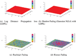
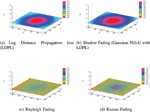
A transmitter is placed at the center of the room and the received signal strength is computed at 3000 points uniformly placed in the small room and 50000 points in the large room. The distance between adjacent points is 0.1m. Figure 1 and 2 shows the signal-space map in the small and big rooms respectively. As expected, the signal profile is a set of concentric disks when only log-distance propagation loss model is used and since the model does not consider any variations due to walls, room shape or presence of objects. Figure 1(b) and 2(b) show the results when shadow fading is present in the same space. The presence of shadow fading without regards for the objects that caused the fading are not expected to show any spatial characteristics of either space. Figure 1(c) and 2(c) used the building propagation loss model with the transmitter placed in the second floor and hence there is no LoS signal. Again, the signal map is more-or-less uniformly random with no specific spatial features or pattern. Similarly, the Rician fading simulated with the transmitter in the first floor shows a strong signal at the center of the room but the general signal profile does not represent specific room geometry or shape. Indoor localization algorithms depend on the spatial features that show up when signal is received and the absence of the features in ns3 simulation makes it unsuitable for evaluating localization algorithms.

Figure 1 Signal map from various loss models in ns3 in a small room (5m × 6m × 5m).

Figure 2 Signal map from various loss models in ns3 in a large room (25m × 20m × 5m).

3.3 Co-Moving and Non Co-Moving Receivers

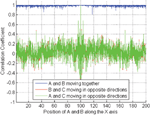
We simulated co-moving receivers in ns3. Two receivers ‘A’ and ‘B’ that started at the same point (0, 0) and moved together were simulated. Similarly we simulated a third receiver ‘C’ that started at (200, 0) and moved toward the first two receivers. The received signal strength at each receiver A, B and C from a transmitter placed in the middle of the room was recorded. Sets of 60 signal strength samples at A, B and C were taken at each position and correlation coefficients of sample sets at the pairs A–B, B–C and A–C are computed. These steps are repeated for each position throughout the trajectory and results for Nakagami and Random fading models are shown in Figure 3. We observe that regardless of how the three transmitters move (together or not), the received signal strengths have no significant correlation. This defies intuition and also contradicts the empirical results obtained by Chandrasekharan et al., [9].

Figure 3 Correlation of signal strengths at receivers moving together and opposite directions using ns3.

3.4 Discussion

The fundamental reason why simulators, such as ns3 [22], are unable to model the realistic spatio-temporal variations is because signal-space characteristics at larger distances such as two receivers in a room, is not understood sufficiently to be mathematically modeled. There has been efforts in wireless communication to model spatial correlation of Rayleigh faded channels [24], however, the models are designed for very close distance such as in multi-antenna and MIMO communication systems. Therefore, one of the research problems that one could solve is to obtain empirical data to understand and model all dependent variables that lead to the signal to space correspondence of signal strength values observed in experiments. Once the phenomenon is understood, multi-variate distributions using Copula [25] theory could be used. However, tremendous amount of measurement efforts will be required to build a robust model of this dependence structure. We describe a computationally easier solution, that is based on ray tracing, in the next section.

4 Randomized Ray-Tracing Simulator

Ray-tracing requires finding several paths through which reflected, refracted and scattered components of a transmission reach the receiver. Ray tracing, combined with RF propagation principles, provides deterministic models of signal propagation that can be site-specific and hence come close to reality. The accuracy of ray-tracing increases with the number of signal paths that are traced [26]. Various AutoCAD tools (such as PlaceTool and iBwave) are available for such estimates and can be used to generate site-specific signal-space maps. In general, the ray-tracing tools are used for network planning and design rather than simulating wireless networks and protocols. Recently, a combination of image processing and ray-tracing was proposed to simulate site-specific signal-space profile for use in indoor localization [27]. It is also possible to use traces from CAD or real experiments as inputs to network simulators.

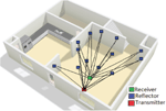
Figure 4 Conceptual diagram of the Ray tracing simulator.

However, this offline/trace driven approach loses accuracy if the network nodes are expected to move around during the simulation which can change the signal-space profile.

We take a middle ground between site-specific information and statistical models to achieve signal to space mapping in hypothetical indoor environments with walls and ceilings while using very little additional computation time. We approximate ray-tracing approaches by randomly selecting a set of points of reflection P on the surface of all obstacles in an indoor space rather than finding points of reflection through brute-force or geometric optics. We assume that the set of points P are where the transmitted signal bounces off just before reaching the receiver. We then compute the distance between transmitter and each p_i∈ P and also from p_i to the receiver. These distances are used to compute the amplitude and phase of the received signal component as described below.

In a multi-path environment the composite received signal is the vector sum of the signals arriving from each path. Assuming that a_ij is the reflection coefficient for surface of the jth reflection of the ith path that arrives at the receiver, then the overall reflection factor is

\begin{array}{r} a_{i} = \prod_{j = 1}^{K_{i}} a_{i j} . & (7) \end{array}

Given that λ is the signal wavelength and $A_{0} = \sqrt{P_{0}}$ where P₀ is the received signal at reference distance d = 1m from of the transmitter, then the amplitude and phase of the received signal at a receiver is a combination of the instantaneous signals arriving from L paths including the direct line of sight signal from the transmitter. If d_i(t) is the distance travelled by the ith path at time t, then

\begin{array}{r} A_{r} (t) = A_{0} \sum_{i = 1}^{L} \frac{a_{i}}{d_{i} (t)} e^{j ϕ_{i} (t)} & (8) \end{array}

\begin{array}{r} ϕ_{i} (t) = - \frac{2 π d_{i} (t)}{λ} & (9) \end{array}

The received power P r(t) at the receiver r at time t is then given by [28]

\begin{array}{r} P_{r} (t) = P_{0} {| \sum_{i = 1}^{L} \frac{a_{i}}{d_{i} (t)} e^{j ϕ_{i} (t)} |}^{2} & (10) \end{array}

In simulations presented in this paper, we use 6 reflectors on each surface and all surfaces have the same reflection coefficient. Therefore, we drop the subscript from a_ij and write the reflection coefficients of the kth reflector on a surface as a^k. We simplify the computation of distance travelled by each path by simply using d_i(t) as the sum of straight line distances from the transmitter to the point of reflection p_i and the distance from p_i to the receiver. In geometric optics, this will be the straight line distance of the receiver from the mirror image of the transmitter (or vice-versa) for the first reflection. Since we choose a different set of points P at every instant of time t, we obtain a time-varying signal at the receiver. This time variation simulates multipath fading due to movements in local environment even if the transmitter and receiver are stationary. Our goal is to simulate stationary indoor environment where Doppler effect plays very little role. Therefore, our simulator does not model the effect of moving transmitters and receivers.

We simulated this approach in MATLAB. We constructed simple clutter-free models of indoor spaces with 6 reflectors created on each of the four walls as well as the floor and the ceiling. We generate 60 sets of such points to simulate time variation. The transmit power is set to 100 mW, transmit and receive antenna gains are 1.64 and 2.65 respectively, the operating frequency is 2.45 GHz and the reflection coefficient of the surfaces is α=−0.7.We present results from various experiments using our ray tracing simulator in the following sections.

4.1 Distance-Power Relationship

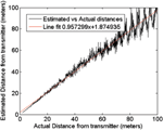
We simulated the distance power relationship in 100m long spaces of various heights and widths. In these simulations, the transmitter height is 3m and receiver height is 1m. The transmitter is located at (0, W idth/2). The receiver is initially located at (0.1,Y/2) and the locations is changed along a line parallel to the X axis at 0.1 m increments. At each new position of the receiver, the received power is computed with the same set of reflectors and an average over 60 readings is computed. There is a straight line of sight component from the transmitter to the receiver in these experiments. The distance power relation is shown in the results presented in Figure 5 along with multipath characteristics. The signal strength fluctuates due to multipath fading which is consistent with empirical data. We fit a curve a + 10 log₁₀x^b to the graph where b is the path loss exponent and a is the path loss at distance 1m. The value of the exponent, with 95% confidence interval, as shown for each figure, varies from ≈1.44 to ≈1.72 while the path loss at the reference distance is between −16 and −17 dBm. In indoor localization applications, such models computed through experiments for a specific indoor setup, is used to estimate distances between a target and fixed reference locations. These distances are used in trilateration algorithms to compute the target location. Therefore, we estimate distances of a receiver placed in various locations in the long narrow alley scenario and plot the Estimated vs Actual distance from the transmitter in Figure 6 and the distance estimation error in Figure 7. We found that with 95% confidence that the error distribution has a Student’s t-distribution with mean –0.266 and standard deviation is 4.97. We further use three transmitters as reference points to compute distances from the powers of signals received from a single receiver. We draw circles with transmitters as centres and the computed distance as radius. We find that for any given room geometry for which we have previously computed the path loss model, we can reliably locate the receiver at the region of intersection of the three circles as shown in Figure 8. There is a 7–10m location estimation error since the absolute location cannot be determined and only a range of possible locations is available. This distance and location estimation error can be reduced by increasing the number of reference points and by using better algorithmic techniques. The experimental results we present here, shows that the randomized ray tracing simulator does not reduce the challenges of inaccurate measurements and hence can replace field experiments in indoor localization research. Thus algorithmic techniques to reduce the localization error can be studied in repeatable simulations using our system rather than spending valuable research hours in tedious measurements.

Figure 5 Distance-power relationship in the randomize ray-tracing approach.

Figure 6 Estimation vs actual distance in a long narrow alley.

Figure 7 Distance estimation error using the ray tracing simulator in a long narrow alley.

Figure 8 Localization using trilateration.

4.2 Spatial Correlation

We experimented with co-located and separately located receivers by simulating three receivers A, B and C. A and B are placed very close to each other (approx 0.01m) near (X = 0, Y = 1, Z = 1) while C is placed at (X = 200, Y = 1, Z = 1). The signal strengths using the ray tracing approach is measured at each receiver. This is repeated for 60 different placements of the reflectors. Same sets of reflectors are used to compute signal strengths at each receiver. The correlation coefficient of the signal samples at the three pairs A–B, B–C and A–C are computed. Next A and B are moved 0.1m toward C and C is moved 0.1m toward A and B along the straight line and the above measurements are taken again using the same set of reflectors and the correlation coefficients are computed. These experiments are repeated until the receivers reach the opposite ends. The correlation coefficients at each position are shown in Figure 9. These results show that the co located receivers experience correlated signal strengths while the signal strengths at separately located nodes has close to zero or negative correlation except at 100m when all three receiver meet in the center of the room. The methodology used in this experiment is similar to the field experiment performed by Chandrasekaran et al. [9] who also presented the same conclusions.

Figure 9 Correlation of signal strengths at receivers moving together and opposite directions using randomized ray-tracing model.

4.3 LOS and Non-LOS Multi-Path Characteristics

We simulated single transmitter-receiver scenarios to obtain statistical characteristics of signal strength in a multipath environment. In this simulation, the transmitter and receivers are at a fixed location and signal strengths at the receiver is computed at one second intervals. We select a new set of reflectors for each second to obtain 60 sample values in mW. We compute the probability distribution of the received signal strengths. Figure 10 shows that the in the absence of Line-of-Sight (nLoS) the signal strengths has a corresponding Rayleigh distribution parameters σ = 0.0021 mW and in the presence of a strong LoS component, the parameters for a Ricean fit is σ = .0016,μ = 3.75. We do not get exact correspondence with the Ricean distribution in the LoS case but the nLoS signal comes close to being a Rayleigh distribution.

Figure 10 Signal envelope showing Rayleigh and Rician distributions.

4.4 Signal-Space Maps

We present the power map in a large and a small room as computed from the randomized raytracing approach. We simulated two room sizes (5m × 6m × 3m) and (25m × 20m × 5m). We placed a transmitter in the middle of each room and obtained signal strengths at various points in the room using the same set of random reflectors. We also compute the average signal strengths over a course of 60 measurements by changing the set of reflectors for every measurement and then taking an average for each point in the simulated space. We used a transmitter in the middle of the room at 2m height to obtain results in LoS environment. For NLoS environment, we place the transmitter at 6m so that it is outside the room and the LoS signal is not used in the calculation of received envelop. Figure 11 shows the results in both LoS and NLoS environment. We see that the received power in the rooms depends on the shape and size of the room. There is clearly higher received power close to the transmitter even in the NLoS environment. Unlike the ns3 results, the signal power is not arbitrarily random throughout the room. The region of high power near the transmitter is elliptical due to rectangular shape of the room rather than circular as in ns3. We expect to see further location dependent characteristics as the room gets cluttered with objects and reflectors are chosen on obstacles other than walls, floor and ceiling.

Figure 11 Signal-power map using randomized ray-tracing simulator.

5 Additional Reference Points for Trilateration

We end the description and characterization of our simulator by presenting results from the affinity propagation technique that can be used to select additional reference points [29] for trilateration based indoor localization. These reference points can be used to compute distances for trilateration and hence improve localization accuracy. We explore the affinity propagation technique which has been proposed for image recognition, finding key sentences in prose and other applications where a set of exemplar or leaders can be used to define the remaining system [29]. In indoor localization, this technique can be applied to select the best nodes that can then be used to find more reference distances for location computation and hence improve location accuracy. We describe the general affinity propagation approach below and present results from our simulator to demonstrate how indoor localization can use this technique to select exemplar devices.

5.1 Affinity Propagation

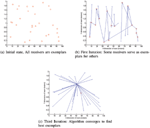
For each pair of devices, the location estimate is used to define similarities between two devices. We define similarities as the negative estimated Euclidean distance between them i.e. s_i,j = −dist(n_i− n_j) where i and j are the device ids and n_i and n_j are their locations. Then “responsibility” matrix r(i, k) ← s(i, k) − max_{k′ ≠ k}{a(i, k′) + s(i, k′)} quantifies how well-suited k is to serve as the exemplar for i, relative to other candidate exemplars for i. The suitability is defined in terms of relative distances between i and other nodes in the sub-region. A nearby device will be a more suitable as an exemplar compared to one that is further away. Similarly, an “availability” matrix a(i, k) ← min(0,r(k, k)+ ∑_{i′ ∉{i,k}} max(0,r(i′,k))) and a(k, k) ← Σ_{i′ ≠ k,}, max(0,r(i′, k)) to represent whether node i would be available to be an exemplar for node k. The availability, in our application, depends on the density of devices in the neighbourhood of each exemplar. In our initial experiment, we started with all nodes as exemplars and with the goal of reaching the minimum number of exemplars. The exemplar set is reduced with each iteration of the affinity propagation algorithm. Results, using our simulator, in a 50 node scenario shows that the algorithm converges in just three iterations (Figure 12(b) and (c)).

Figure 12 Using affinity propagation to elect an exemplar device, ‘O’ denotes exemplars, ‘x’ denotes other nodes, edge between a node and an exemplar indicates the exemplar’s responsibility to the node.

6 Conclusion

We have presented a technique to implement more realism in network simulations. Our technique produces signal distribution characteristics similar to statistical models that were built in the past. We were also able to simulate correlated errors in close spaces by showing correlated fading for co-moving receivers. In the future, we propose three research directions. First a comparison with geometric optics and brute-force techniques to understand the amount of realism that we forsake by randomizing the selection of reflectors. Second, a measurement campaign to obtain spatio-temporal map of signal strengths in an indoor space to gather statistics such as correlation of signal at similar spaces such as corners and around obstacles. Third direction is to evaluate the effect and utility of incorporating our model in various wireless network simulation studies.

References

[1] Zeng, X., Bagrodia, R., and Gerla, M. (1998). “Glomosim: a library for parallel simulation of large-scale wireless networks,” in Parallel and Distributed Simulation. PADS 98. Proceedings. Twelfth Workshop (Rome: IEEE), 154–161.

[2] McCanne, S., Floyd, S., Fall, K., Varadhan, K., et al. (1997). Network simulator ns-2.

[3] Kotz, D., Newport, C., Gray, R. S., Liu, J., Yuan, Y., and Elliott, C. (2004). “Experimental evaluation of wireless simulation assumptions,” in Proceedings of the 7th ACM International Symposium on Modeling, Analysis and Simulation of Wireless and Mobile Systems (New York, NY: ACM), 78–82.

[4] Haq, F., and Kunz, T. (2005). “Simulation vs. emulation: Evaluating mobile ad hoc network routing protocols,” in Proceedings of the International Workshop on Wireless Ad-hoc Networks (IWWAN 2005).

[5] Takai, M., Martin, J., and Bagrodia, R. (2001). “Effects of wireless physical layer modeling in mobile ad hoc networks,” in Proceedings of the 2nd ACM International Symposium on Mobile Ad Hoc Networking & Amp; Computing, MobiHoc ‘01 (New York, NY: ACM), 87–94.

[6] Lee, H., Cerpa, A., and Levis, P. (2007). “Improving wireless simulation through noise modeling,” in Information Processing in Sensor Networks, IPSN 6th International Symposium (Rome: IEEE), 21–30.

[7] Mcdougall, J. M. (2004). Low complexity channel models for approximating flat Rayleigh fading in network simulations. PhD thesis, Texas A&M University.

[8] Martin, E., Vinyals, O., Friedland, G., and Bajcsy, R. (2010). “Precise indoor localization using smart phones,” in Proceedings of the international conference on Multimedia, MM ‘10, 787–790.

[9] Chandrasekaran, G., Ergin, M. A., Gruteser, M., Martin, R. P., Yang, J., and Chen, Y. (2009). Decode: Exploiting shadow fading to detect comoving wireless devices. Mobile Comput. IEEE Trans. 8, 1663–1675.

[10] Walfisch, J., and Bertoni, H. L. (1988). A theoretical model of UHF propagation in urban environments. Antennas Propag. IEEE Trans. 36, 1788–1796.

[11] Torres, R. P. Valle, L. Domingo, M. and Diez, M. C. (1999). Cindoor: an engineering tool for planning and design of wireless systems in enclosed spaces. Antennas Propag. Mag. IEEE 41, 11–22. doi: 10.1109/74.789733

[12] Honcharenko, W., Bertoni, H. L., Dailing, J. L. Qian, J., and Yee, H. D. (1992). Mechanisms governing uhf propagation on single floors in modern office buildings. Vehicular Technol. IEEE Trans. 41, 496–504. doi: 10.1109/25.182602

[13] Seidel, S. Y. and Rappaport, T. S. (1994). Site-specific propagation prediction for wireless in-building personal communication system design. Vehicular Technol. IEEE Trans. 43, 879–891. doi: 10.1109/25.330150

[14] McKown, J. W. and Hamilton, R. L. Jr. (1991). Ray tracing as a design tool for radio networks. Network IEEE 5, 27–30. doi: 10.1109/65.103807

[15] Tan, S. Y. and Tan, H. S. (1996). A microcellular communications propagation model based on the uniform theory of diffraction and multiple image theory. Antennas Propag. IEEE Trans. 44, 1317–1326. doi: 10.1109/8.537325

[16] Kouyoumjian, R. G. and Pathak, P. H. (1974). A uniform geometrical theory of diffraction for an edge in a perfectly conducting surface. Proc. IEEE 62, 1448–1461. doi: 10.1109/PROC.1974.9651

[17] de Adana, F. S., Gutierrez Blanco, O., Diego, I. G. Perez Arriaga, J., and Catedra, M. F. (2000). Propagation model based on ray tracing for the design of personal communication systems in indoor environments. Vehicular Technol. IEEE Trans. 49, 2105–2112. doi: 10.1109/25.901882

[18] Seidel, S. Y. and Rappaport, T. S. (1992). A ray tracing technique to predict path loss and delay spread inside buildings. In Global Telecommunications Conference, 1992. Conference Record., GLOBECOM ‘92. Communication for Global Users, IEEE, vol. 2, 649–653.

[19] Heidemann, J., Bulusu, N., Elson, J., In-tanagonwiwat, C., Lan, K., Xu, Y., Ye, W., Estrin, D., and Govindan, R. (2001). Effects of detail in wireless network simulation. In Proceedings of the SCS Multiconference on Distributed simulation, 3–11.

[20] Sohn, T., Li, K. A., Lee, G., Smith, I., Scott, J., and Griswold, W. G. (2005). Place-its: A study of location-based reminders on mobile phones. in UbiComp 2005: Ubiquitous Computing, volume 3660 of Lecture Notes in Computer Science eds M. Beigl, S. Intille, J. Rekimoto and H. Tokuda (Berlin: Springer), 232–250.

[21] Aalto, L., Gothlin, N., Korhonen, J., and Ojala, T. (2004). Bluetooth and wap push based location-aware mobile advertising system. In Proceedings of the 2nd international conference on Mobile systems, applications, and services, MobiSys ‘04, 49–58.

[22] Riley, G. F., and Henderson, T. R. (2010). The ns-3 network simulator. in Modeling and Tools for Network Simulation (Berlin: Springer), 15–34.

[23] Rappaport, T. S. (2002). Wireless communications: principles and practice.

[24] Al-Hussaibi, W., and Ali, F. H. (2012). Generation of correlated rayleigh fading for accurate simulation of wireless comm systems. Simul. Model. Pract. Theory 25, 56–72. doi:10.1016/j.simpat.2012.01.009

[25] Durante, F., and Sempi, C. (2010). “Copula theory: an introduction,” in Copula Theory and Its Applications, eds P. Jaworski (Berlin: Springer), 3–31.

[26] German, G., Spencer, Q., Swindlehurst, L., and Valen-zuela, R. (2001). “Wireless indoor channel modeling: statistical agreement of ray tracing simulations and channel sounding measurements,” in Acoustics, Speech, and Signal Processing, 2001. Proceedings.(ICASSP 01), IEEE, vol. 4, 2501–2504.

[27] Ji, Y., Biaz, S., Pandey, S., and Agrawal, P. (2006). “Ariadne: a dynamic indoor signal map construction and localization system,” in Proceedings of the ACM MobySys (New York, NY: ACM), 151–164.

[28] Pahlavan, K. and Levesque,A. H. (2005). Wireless Information Networks, volume 93. New York, NY: Wiley.

[29] Frey, B. J., and Dueck, D. (2007). Clustering by passing messages between data points. Science, 315, 972–976.

Biographies

S. Jain is an Assistant Professor in the Mathematics and Computer Science department at York College of CUNY and a Doctoral faculty of Computer Science in The Graduate Center of CUNY. She received her BE degree in Electronics and Telecommunication Engineering from Bengal engineering college in 2001, and MS and Ph.D. in Computer Science from Stony Brook University in 2005 and 2007. She is a senior member of the IEEE and her research interests are in mobile and wireless communication and networks.

C. J. Barona is an Assistant Control Engineer in the Capital Program Management Department at New York City Transit. He received his BE degree in Electrical and Electronics Engineering from The City College of New York – CUNY in May 2015. His Senior Design Project was mainly focused on wireless communications technologies. During his last year as an undergraduate student, he worked closely with Professors Shweta Jain, and Nicholas Madamopoulos in development of a low cost ray tracing technique that was capable of modeling multipath effects and signal interferences for indoor space environments. He participated as one of the co-authors in the IEEE 36th Sarnoff Symposium held in New Jersey, where he spoke about the latest progress of his publication “Modeling Realism in Wireless Simulations”. In January 20th of year 2016, He became a Certified Engineer from State of New York by successfully passing his F.E exam. His research interests are wireless communication, control and automation engineering.

N. Madamopoulos received the B.S. degree in Physics (with honors) from the University of Patra, Greece, in 1993 and the M.S. and Ph.D. degrees in Optical Science and Engineering from CREOL/College of Optics and Photonics, University of Central Florida, Orlando, in 1996 and 1998, respectively. His Ph.D. specialization was in photonic information processing systems, where he introduced novel photonic delay lines for phased array antenna applications, as well as photonic processing modules for fiber-optic communications.

His research interests include optics and photonic systems for information processing in telecom and non-telecom applications. He has held several positions in Academia (Hellenic Air Force Academy, City College of New York, University of California-Santa Barbara, The College of Optics and Photonics-CREOl, the National Hellenic Research Foundation). He has also spent many years conducting research for the industry, where he served as Sr. Research Engineer for Calient Networks, Inc. (Santa Barbara, CA), Member of Technical Staff for Lucent-Bell Labs (Somerset, NJ), and Sr. Research Scientist for Corning, Inc. (Corning, NY and Somerset, NJ). Dr. Madamopoulos is a Senior Member of IEEE-Photonics Society. He was one of the founding members of the first IEEE-LEOS Student chapter (Orlando Chapter) and he served as treasurer and president for several years. He received a New Focus Student Essay Prize in 1996, the SPIE Educational Scholarship in Optical Engineering in 1997, the Graduate Merit Fellowship Award in 1998 and the New Focus/OSA Student Award in 1998.