Enhanced Ant Colony-Inspired Parallel Algorithm to Improve Cryptographic PRNGs

Jörg Keller¹, Gabriele Spenger^1,* and Steffen Wendzel²

¹FernUniversität in Hagen, Germany
²Worms University of Applied Science, Germany

Email: joerg.keller@fernuni-hagen.de; gabriele@spenger.org; wendzel@hs-worms.de

*Corresponding Author

Abstract

We present and motivate a parallel algorithm to compute promising candidate states for modifying the state space of a pseudo-random number generator in order to increase its cycle length. This is important for generators in low-power devices where increase of state space to achieve longer cycles is not an alternative. The runtime of the parallel algorithm is improved by an analogy to ant colony behavior: if two paths meet, the resulting path is followed at accelerated speed just as ants tend to reinforce paths that have been used by other ants. We evaluate our algorithm with simulations and demonstrate high parallel efficiency that makes the algorithm well-suited even for massively parallel systems like GPUs. Furthermore, the accelerated path variant of the algorithm achieves a runtime improvement of up to 4% over the straightforward implementation. This publication is an extended version of [10].

Keywords

Pseudo-Random Generators
Parallel Efficiency
Ant Colony
Lightweight Cryptography

1 Introduction

Pseudo-random numbers are an important ingredient in a wide range of cryptographic protocols and applications, including applications in resource-constrained environments such as RFID chips or Internet of Things. There, the pseudo-random number generators (PRNGs) can only use little energy, i.e. use simple algorithms, but still must provide a decent level of security.

For instance, in smart sensors or wearables, limited computing power and solar-powered energy-supply challenges the implementation of state-of-the-art cryptographic algorithms. With the increasing number of field-deployed but soon to be obsolete IoT components, this problem can be expected to increase. One of the important criteria for a PRNG is the cycle length, i.e. the number of outputs until the sequence of outputs will repeat, but there are more criteria such as good statistical properties of the output sequence, forward and backward secrecy to name a few. Hence it is quite complicated to design a PRNG with a moderate state space size (because of resource constraints such as energy from a battery) that can provide these properties. For a PRNG that has already been investigated with respect to above criteria but where an increase in cycle length is desirable, we have proposed in previous work a method that only modifies a small number of state transitions to increase cycle length notably [18]. In order to find which state transitions to change, the state space of the PRNG has to be sampled, which is computationally intensive, and thus calls for the use of parallel computing.

In this work, we motivate and present a parallel algorithm to find promising states, called candidate states, for the modification of state transitions. The parallel algorithm is inspired by the behavior of ants, that tend to follow trails where other ants have already passed. We demonstrate the advantage of our algorithm over a straight-forward parallel implementation by simulation. While the asymptotic parallel efficiency of the parallel algorithm is highly dependent on the structure of the state transition graph, experiments indicate a good parallel efficiency (70%) in practice even for 1000 threads. Thus, together with its regular structure, the algorithm is suited for massively parallel computing engines like GPUs.

The remainder of this paper is organized as follows. In Section 2, we summarize background information on PRNGs. In Section 3, we present a parallel algorithm to identify promising candidate states for transition modification. In Section 4, we demonstrate the suitability of our parallel algorithm by simulation experiments. In Section 5, we describe further improvements to achieve longer cycles. Section 6 gives conclusions and an outlook to future research.

2 Fundamentals & Related Work

Pseudo-random number generators (PRNGs) are used to generate (pseudo-) random numbers that are frequently used in communication protocols, be it as a nounce, a challenge, or for some other purpose. Between seedings, and while no additional entropy bits are input to the PRNG, on each call it outputs a value that depends on the current state, and transitions to a follow-up state by applying a state transition function on the current state. Thus, it works like a finite state automaton without input. A hash chain, i.e. a cryptographic hash function repeatedly applied to some initial value, is also used in cryptographic protocols, e.g. in Lamports authentication protocol [12]. After hashing the initial value once, the hash function works on the set of hash values much like the above transition function on the set of states. Other cryptographic primitives such as stream ciphers might be modelled in this manner as well.

PRNGs in resource-constrained systems such as mobile sensors typically use a state space of moderate size, because e.g. in 8-bit systems the increase of the state space by 8 bits leads to one more instruction for each addition or logical operation, which in turn increases the energy consumption per cryptographic operation, and thus puts a load on the battery. Hence we see hash functions with low computational load and 64-bit output like SipHash https://131002.net/siphash/siphash.pdf or BLAKE2s see RFC 7693., and PRNGs with state spaces of similar size, such as AKARI [14].

There are a number of general security requirements for cryptographic primitives like forward secrecy and backward secrecy [15] and PRNG-specific models such as [3] and [4], or suites that test the output of PRNGs for randomness such as the Marsaglia suite of Tests of Randomness [13] and the NIST test suite [17]. Still, if the cycle length of the primitive is short, patterns of output bits can be stored and repetition can be detected. A practical example for this is the attack on A5/1 (cf. [2, 7]). Thus, a long cycle length is a prerequisite for enabling forward secrecy.

A PRNG can be modelled as a deterministic state transition function f : M → M mapping a finite state space of size n = |M| to itself. If a single state is interpreted as a node and the transition between a state and its unique successor state is interpreted as an edge, the result is a directed graph G_f = (V ;E) with V := M and E := {(x, f(x))|x ∈ M}, where each node has exactly one outgoing edge (deg-1 graph). The structure of the generated graph provides information about the behavior of the primitive. For non-bijective transition functions, the graph typically consists of several weakly connected components. Each of these components consists of one cycle and generally several trees with roots located on the cycle. The trees tend to be very ragged. Figure 1 depicts the structure of a component.

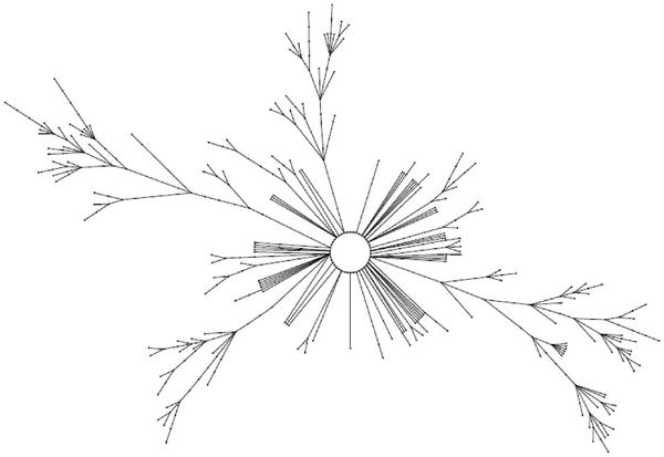
Figure 1 Typical connected component of a state transition graph, taken from [1].

Properties of the graph include the number and sizes of the connected components, length of the cycles and maximum depth of the trees. In order to identify all connected components of a graph, the complete state space would have to be analyzed, e.g. by a depth first search (DFS). The cycles can be detected by starting from the unique back edge in each component. If the state space is too large for complete exploration, a part of the state space can be analyzed, accepting the fact that one or several components might be missed. Still, this approach can provide valuable information about the expected state space structure. The typical approach is to randomly select nodes as starting points, and to follow the path from each starting point until a cycle is reached. The number of followed paths, which influences analysis time, does not need to be very large: as the expected number of components is small (see below), already a small number of sample paths through the state graph will hit all of the larger components, and provide their cycle lengths. Please note: as the components are much larger than their cycles, a short cycle in such a component affects many seed states in the state graph.

In [9], an analysis method of the state space is presented that avoids the large memory requirements of depth-first search, where each node must be marked as visited, which is clearly impossible if n ≥ 2⁴⁰. The idea is to only store certain nodes while traversing the tree. If only the nodes are stored that are reached after 2, 2², 2³, … steps taken since the start value (so called anchors), the required memory usage is logarithmically in the number of steps, i.e. O(log n), and thus very low. A cycle is reached if the newest anchor is reached again. Figure 2 illustrates the process of cycle detection. The low memory requirement comes with a time overhead: the algorithm might need twice as long as would be needed in the optimal case.

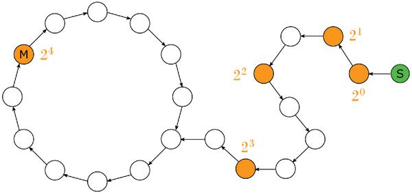
Figure 2 Cycle detection.

This runtime can be improved by spending more memory, but less than 1 bit per node. One can store the nodes reached after k, 2k, 3k, … steps, and check in each step if one of the stored nodes is reached again. This reduces the overhead to at most k additional steps, but requires a search data structure of size M = O(m/k) for a path of length m, which must be queried in each step. Hence, the query time must be constant (at least if amortized over many queries), for example by using a hash table with low utilization. The parameter k can be chosen given the path length m and the memory size M. While the latter is known for the computer to be used, the path length can only be guessed. For a randomly chosen state transition function, the expected path length is $O (\sqrt{n})$ [6]. However, there is no guarantee for this, so if the data structure runs out of memory, it must adapt dynamically by throwing away every other node stored, and increasing k to twice its former value. The data structure can also be used to shorten the time for sampling further paths: if one keeps the nodes stored from previous paths, then one can stop following a further path if one of these stored nodes is reached. Because of the tree structures in the components (cf. Figure 1) the paths meet sooner or later in the tree. At least, if two paths are in the same component, another complete walk around the cycle can be avoided for the second path. As both the expected tree path The tree path is the path from the start node until the entry into the cycle. and cycle lengths are $O (\sqrt{n})$ with comparable constant factors [6], this on average should reduce the length by a factor of 2. As the number of weakly connected components is expected to be small (0.5log n, see [6]) with one component expected to dominate (0.75n), many paths will be in the same components, and thus it normally pays off to increase k to be able to store nodes from all paths sampled so far.

The runtime of this algorithm is proportional to the average length of the paths and the number of starting points. As a small number of starting points suffices, the average path length can be around 2⁴⁰ and still yield reasonable analysis time. This restricts n to 2⁸⁰ if path lengths are around $\sqrt{n}$ (see above), which allows analysis of PRNGs or hash chains on a 64-bit state space. The resulting tree and cycle structure for these samples might provide valuable insights with respect to the security of the algorithm. Also, the sizes of the connected components can be guessed from the fractions of starting points belonging to each component, within a confidence interval. Please note that there are comparable approaches for bijective functions, notably Knuth’s algorithm [11] with an expected runtime of O(n log n), which can be made linear in time by using 1 bit per node, or improved by using stored nodes as described above.

3 Algorithms

For a PRNG with a short cycle, our strategy to increase the cycle length is to cut the cycle at some node (which we will call a special state in the following) by modifying the transition function to divert to a node somewhere deep in the tree [18], as illustrated in Figure 3. There, the outgoing edge (u_i, w_i) of cycle node u_i is modified, and tree node v_i becomes the new successor of u_i. The resulting cycle length will be the sum of the previous cycle length and the length of the tree path from v_i to w_i. This modification of the state transition graph will be called “Action A” in the following.

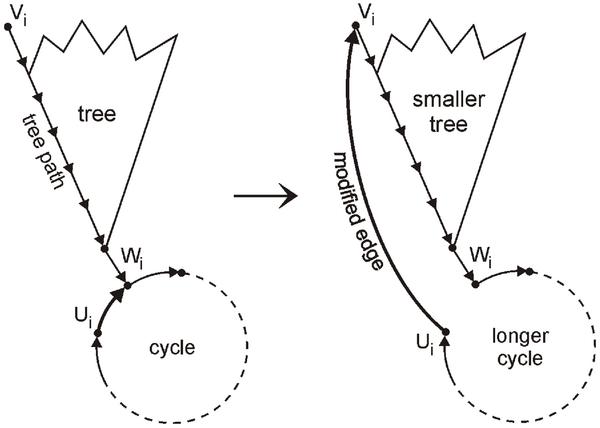
Figure 3 Breaking up a cycle to increase cycle length.

This can be done for each component of notable size, and even multiple times within each component to achieve a larger increase of the cycle length Also other modifications can be applied: see Section 5 and [18].. As the number of components is expected to be small, with only a few components of notable size (see previous section), the total number of modified edges will be small as well, and can be stored in a lookup table. The modified PRNG state transition function can then be implemented as given by Algorithm 1.

Algorithm 1 Modified state transition function.

images

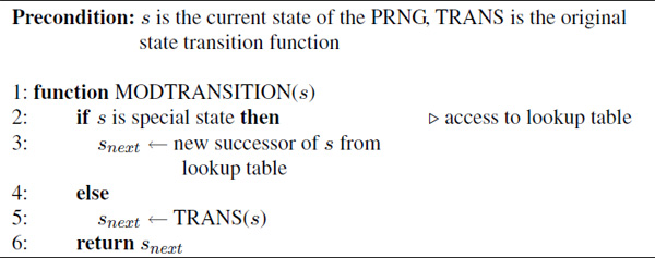
Please note that the time spent in the lookup table still increases the execution time of the transition function, which could increase the energy consumption. Hence, we split the test — which will fail most of the time, because there are only few special states — into two parts: a very fast test, that fails in most cases, and a follow-up test, that does the exact check but is executed only seldomly. The first test uses a property that is easily testable, e.g. that some bits of the state representation have a certain bit pattern. We call these nodes candidates. The only restriction imposed by this test is that states where the transition function shall be altered must be candidates, which is however no serious restriction, cf. [18].

The difficult task is to find a small number of special states and new edges going out from these special states. This must be done such that cycle lengths are increased and other properties like statistic behavior of output is not harmed. While this has to be done only once, i.e. is an oﬄine task, it requires to sample the state graph (see previous section), i.e. it might require 2⁴⁰ executions of the state transition function if the average path length is 2³² and 2⁸ starting points are chosen. To do this in a reasonable time calls for a parallel algorithm.

If we ignore the case of encountering a component without a candidate (that case can be handled by additionally using anchors, cf. Section 2), then the selection of special states can be done using the construction of the candidate graph, i.e. the graph of all candidate nodes reachable from the chosen starting points. An edge in the candidate graph between two candidate nodes c_i and c_j represents the unique path in the state graph from c_i to c_j, and is annotated with the length of this path. When the candidate graph has been computed, the cycle lengths and the tree depths can be computed by DFS as the candidate graph is much smaller than the state graph and will fit into the memory. The special states can be chosen by changing edges such that the increase in cycle length is maximized. This can be repeated until all candidates of a connected component of the candidate graph are on a cycle, or a maximum number of special transitions is achieved. For further details about the determination of special states from the candidate graph, see Section 5 and [18].

The computation of the candidate graph follows a simple paradigm: the paths originating from the starting points are followed, and if two paths meet, only one of them is followed further. While we are following a path, we record all candidates that we visit. This leads to the following basic parallel algorithm, cf. Algorithm 2.

Algorithm 2 Parallel algorithm to compute candidate graph.

images

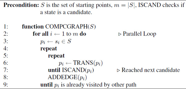
Each thread follows a path from one candidate to the next. Then it checks if that candidate has been already visited by another thread. If so, then the thread stops, and the other thread continues. If not, then the thread follows this path further in the next round. If two threads reach a candidate in the same round, then the one with the smaller ID continues. Please note that we hide some details here. First, to construct the candidate graph, not only nodes but also edges with distances must be added. Also, one thread will reach the cycle and there meets a candidate visited earlier by itself, which must also be detected. Finally, it is not guaranteed that a path contains a further candidate (although this is unlikely), so that in addition, other measures are necessary to detect if a cycle has been reached (cf. Section 2).

The parallel algorithm partitions each tree in the graph into chains that correspond to the paths that the threads follow. A chain always starts in a starting point s_i and ends in a candidate reached by more than one path and where s_i is not the closest starting point. Put otherwise, when the path from s_i reaches the candidate, it has been visited before by another thread. Figure 4 illustrates this with five starting points A to E, where the paths starting in A and B meet in candidate X, and only the path from A is followed further. Similarly, the paths starting in C, D and E meet in candidate Z, where only the path from C is followed further until candidate Y, where it meets the path from A, that is followed further around the cycle. The different chains are indicated by different colors.

Figure 4 Parallel sampling of paths.

The runtime of the algorithm is then determined by the longest chain, i.e. by the longest sequence of candidates found from this set of starting points, multiplied with the average distance between candidates. The average distance between candidates is n/c if there are n possible states and c candidate states, assuming that the transition function is random enough that the deterministic choice of the candidates makes their distribution in the graph similar to a random distribution. The standard deviation is high, however, so that the maximum distance occurring in one round can be much higher than the average, leading to load imbalance and idling threads. In order to avoid this, each thread follows several paths in each round, so that the resulting runtime better approaches the average. In addition, this occurs quite naturally as the number of followed paths m can be larger than the number p of threads available, even considering a massively parallel environment like a GPU with several thousand hardware threads. The technique to follow multiple paths per round with subsequent query for visited candidates has been used before in a parallel program [8], although with a different intention: by bundling multiple queries and querying more seldom, the high communication cost in a message-passing machine could be amortized. This does not play a role in our current research as the graph is small enough to be kept in a shared memory. Still, in a GPU, the access to the global memory is slow, so that infrequent coordinated access helps performance.

If the number of followed paths gets smaller after some time, a load balancing can be performed to handle load imbalance as far as possible. As soon as the number of followed paths gets smaller than the number of threads, a load imbalance necessarily occurs. This load imbalance hurts if the difference between the maximum chain length and the majority of chain lengths is large. As the small example in Figure 4 illustrates, after two rounds only two of the five chains are left, and after three rounds only one chain is left, which continues for another four rounds.

The runtime could be improved if such long chains could progress faster relative to other paths. Note that this is possible as a thread follows several paths in each round, so that instead of advancing t paths to the next candidate, the thread could advance t - 2 paths to the next candidate and one path to the next but one candidate. Thus, the latter path would progress twice as fast as the other paths. As the thread now only handles t - 1 instead of t paths, a different distribution of paths onto threads is necessary, but presents no problem. Unfortunately, the long chains are only known at the end of the algorithm, so it is not clear which path should progress faster than the others.

In order to still improve load balance, we borrow an analogy from nature: when an ant meets the path of other ants, it tends to follow this path, thus strengthening this path by placing further pheromone. Ant colony algorithms have successfully been used to solve problems related to graph theory, e.g. in [5]. Here, if a path meets a candidate that has been already visited by another path, it strengthens that path by “donating” its own time slot to the other path, which is possible as the first path need not be followed further. Hence, if the other path is a long chain, it will progress faster. While this simple heuristic will not help a long chain where no other paths end, that situation is unlikely due to the ragged structure of the trees in random deg-1 graphs. Obviously, this donation cannot be continued long in a linear fashion, because each thread follows at most m/p paths in one round, and therefore an acceleration of a path that got donations from more than m/p others would slow down a round. Hence, the most advantageous form of acceleration must be found out by experiments, as the optimum acceleration cannot be determined at runtime. Furthermore, the donation can be transitive, i.e. a path that got donations from other paths, and donates its own time to another path, would also donate the time it got itself from others.

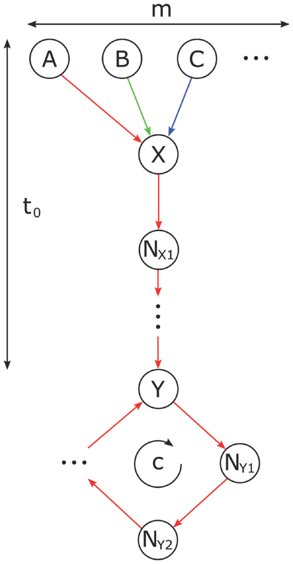
Figure 5 Candidate graph with minimum parallelization potential.

To motivate the concept of donation further, let us assume we start from m starting points and explore the candidate graph from there. If the candidate graph comprises q nodes after exploration, and we employ p ≤ m processors, then a trivial lower bound is q/p steps, where a step represents the (average) time to bridge the distance between two candidate nodes. Another lower bound arises from the structure of the candidate graph. If the shortest path from a starting point to the first candidate on the tree comprises t₀ candidate nodes, and the cycle comprises c candidate nodes, then the minimum runtime of any (sequential or parallel) algorithm is t₀ + c. Consequently, the processors cannot be fully used, leading to low parallel efficiency, if q/p < t₀ + c, i.e. if p > q/(t₀ + c). The extreme case happens if all m starting points have a common successor candidate, from which a single path leads to the cycle (see Figure 5).

In such a graph, q = m + t₀ + c, and at most p = 1 + m/(t₀ + c) processors can be employed. As t₀ and c can be assumed to be around $\sqrt{n}$ , and m normally is smaller, this would restrict us to using p = 2 processors.

However, even if q/p is the sharper lower bound, it is not obvious how to balance the load onto the processors, because the lengths of the different chains are unknown. In the (hypothetical) case where we would know all chain lengths h_i in advance, we could proceed as follows. The processors would still work in rounds, but not all chains would be processed with the same speed. By speed, we here mean the number of links in the chain to be processed in one round. The speed of chain i would be proportional to h_i/q, as ∑_ih_i = q, so that if a chain is twice as long as another, it gets processed twice as fast. In this manner, all rounds could be completely filled, and all processors employed, as all chains would be completely processed at the end. We admit that we simplify a bit, because the workload must still be distributed over the processors, and non-integral values of h_i/q must be handled, but both issues are more technical than challenging. Figure 6 depicts that the chain lengths in practice indeed vary widely. For candidate graphs of the logistic function and MD5, both with 10, 000 starting points, the distributions of chain lengths in the largest connected component are shown.

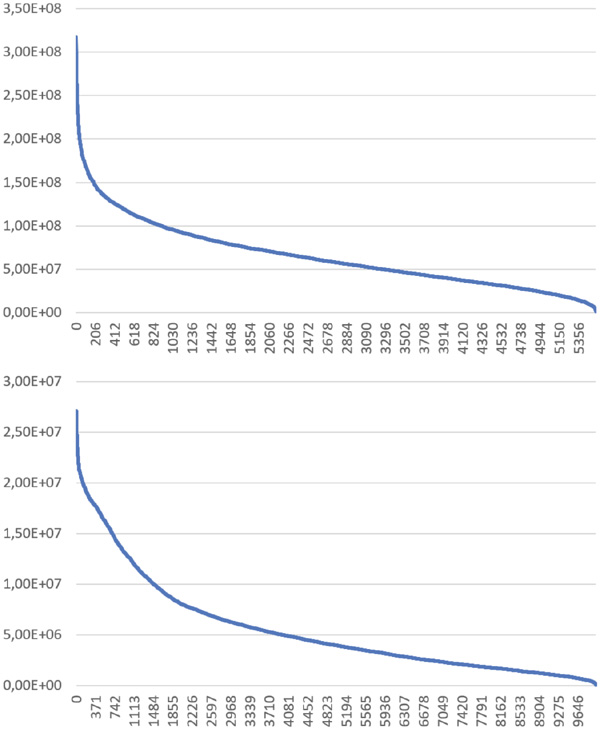
Figure 6 Chain lengths of Logistic Map (above) and MD5 (below).

The consideration of the hypothetical case shows that in order to have a parallel algorithm with high parallel efficiency, it is best to process long chains faster than short ones. In our real case, we do not know anything about the length of the chains initially, we just know the starting points. When following the chains, some will terminate early. This means, that they have been processed too fast, and the others too slow. This motivated the donation strategy to accelerate the processing of long chains. The simplest indicator to identify a potentially long chain is the fact that the chain reached a candidate earlier than another.

The experiments in Section 4 illustrates that simple strategies are sufficient to turn this nature-inspired analogy into a real advantage.

4 Experiments

To quickly assess the advantage of our parallel algorithm with path acceleration over the straight-forward parallel implementation, we use a simulator. The simulator reads in a candidate graph that has been produced in our previous research [18]. It then simulates the threads one by one and round by round. As the candidate graph structure is already available, the inner repeat-until loop from Algorithm 2, that searches for the next candidate, can be reduced to one step. Still, as the distance between succeeding candidate nodes is stored in the graph, the exact runtime of a round (in terms of maximum number of calls to function trans per thread) can be given.

The simulator is applied to a graph with paths from m = 10⁴ randomly chosen starting nodes, using as transition function the cryptographic hash function MD5 with output restricted to 64 bits We are aware that MD5 is outdated, and used SHA-3 in [18]. Both graph structures are quite similar to random deg-1 graphs, and thus should behave similarly with respect to the parallel algorithm.. The candidate set was defined as the set of nodes with bits 4 to 25 set to 1.

The simulator is run in several configurations: either with p = 100, 500 or 1000 threads, to test differing ratios of m/p. We use two simple donation functions: either linear or logarithmic in the number of donated time slots (up to m/p). Additionally, we use the straight-forward implementation, where no donation occurs. For comparison, we also give the sequential runtime. Please note that by runtime, we mean the number of edges from one candidate to the next that a thread follows during the algorithm. We skipped the more exact measure of calls to function trans in order not to model the load balancing.

Table 1 Simulated runtimes of parallel algorithm for different thread count and donation strategies

	Donation Strategy
p	No	Linear	Logarithmic
1	155, 524	–	–
100	1, 614	1, 553	1, 598
500	379	371	380
1000	226	225	229

Table 1 presents the results for the different configurations. We see that for p = 100, the linear donation strategy brings a runtime advantage of 4%, which seems small but is notable given that less than 100 rounds are done in the parallel algorithm, so that it will take a while before time slot donation can show effect. Also, for an algorithm with a sequential runtime of many hours, this increase still saves a minute in the parallel version. For larger p, the advantage is smaller, as more edges have already been processed before the donation can show effect. The logarithmic donation strategy brings a small advantage for p = 100 but is slightly slower than the straight-forward implementation without time slot donation. Hence, the linear donation strategy should be chosen. We also note that the parallel efficiency of our algorithm is high: still 70% for p = 1000, demonstrating scalability for massively parallel computing engines like GPUs. While it would be desirable to formulate parallel efficiency as a function of p, this is not possible as it also depends on the structure of the state graph.

Figure 7 shows the average cycle length of this reduced version of MD5 after a repeated application of Action A with 100 iterations. It can be seen that a significant increase in average cycle length is achieved.

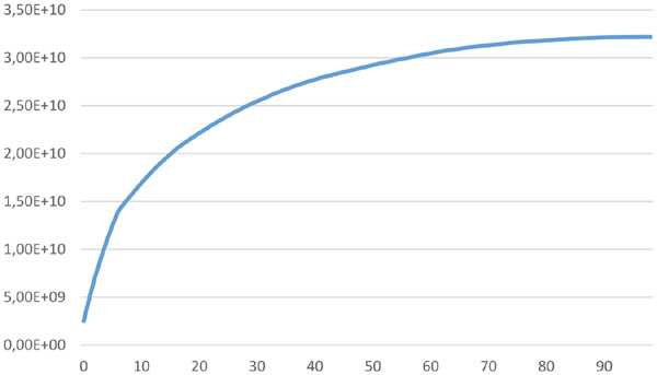
Figure 7 MD5 cycle length after repeated Action A application.

We also tested the algorithm with the logistic map f(x) = a ⋅ x ⋅ (1 - x) for a = 3.99 and x implemented by double precision IEEE754-compliant arithmetic, as an example of a chaotic PRNG [18], but that graph is too small and too flat. It comprises only 20, 295 edges outside cycles for 10, 000 starting points. Thus, no runtime difference between the different donation strategies could be observed. However, the parallel efficiency of the algorithm is high: 99% for p = 100 to 88% for p = 1000.

5 Further Improvements

The results presented in Section 4 show that the gain in average cycle length by the repeated application of Action A saturates after a certain number of iterations. This can easily be explained: let us assume that the initial tree path that is selected for Action A has a length of t₀ and the cycle length of the respective component is c₀. Then it applies that c_i+1 = c_i + t_i, as the cycle length increases by the former tree path and t_i+1 = α ∗ t_i with 0 < α < 1 if we assume as a simplification that the remaining, smaller tree has a depth that is only a fraction α of the previous depth. Solving these equations leads after s iterations to c_s+1 = c₀ + t₀ + t₁ + ... + t_s and t_i = t₀ ∗ αⁱ, which is a partial sum of a geometric series and therefore c_s+1 = c₀ + t₀ ∗ (1 - α^s+1)/(1 - α).

As c₀ and t₀ are typically similar in size, the first iterations increase the cycle length by a factor of two. Subsequent iterations lead to an increasingly smaller growth of the cycle length. In the case that t₀ is significantly smaller than c₀, the growth is even smaller. Using the data from the experiments in 7, the α value was calculated to be ∼0.94 in average, while c₀/t₀ was ∼1.045.

In order to increase the cycle length growths again, a different method for the break-out that is based on two known components i and j can be applied. If one of the components has a significantly larger cycle length c_i > c_j, the components can be joined by breaking up the cycle of the smaller component and break-out to the deepest known tree node of the larger component. This will transform the smaller component into a partial tree of the larger component. As a result, the average cycle length of the state space graph is increased, because the smaller cycle length has been eliminated. The cycle length of component i would be unchanged, but its size would grow to ñ_i = n_i + n_j. The node with the longest tree path would be ṽ_i = v_j, with a tree path length of

{\tilde{t}}_{i} = t_{i} + c_{j} + t_{j} . (1)

As as result, the average cycle length would increase by

M_{i, j} = c_{i} ({\tilde{n}}_{i} - n_{i}) / n - c_{j} n_{j} / n = (c_{i} - c_{j}) n_{j} / n . (2)

Figure 8 depicts the approach, which will in the following be denoted as “Action B”. Please note that Action B increases the tree depth of the larger component, so that subsequent Actions A can improve the cycle length better again.

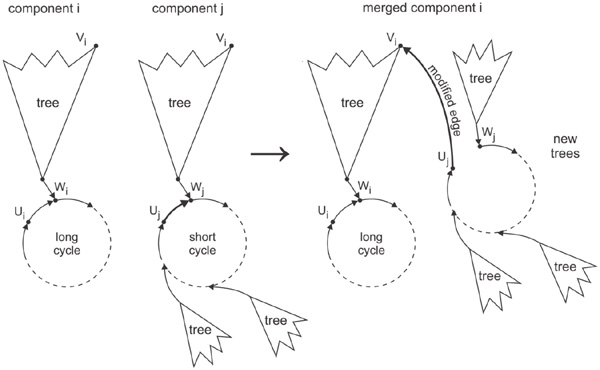
Figure 8 Merging two components.

Figure 9 shows the average cycle length over the number of iterations for Action A only (blue dashed graph) over the combination of Action A and B (red solid graph) for the reduced version of MD5 used in the previous section. Action B is applied as often as possible, i.e. twice for the 100 starting points, as it merges two components that have been identified. It can be seen that the increase in average cycle length by Action B is not very large, however the following Action A produces a notable increase, because a much deeper tree is available. This is expected, because if component i is increased in size in one step by Action B, the maximum tree path length is increased significantly at the same time, so that i will be a good candidate for Action A in the next steps.

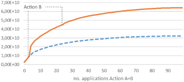
Figure 9 MD5 cycle length after repeated Action A and B application.

After 99 iterations and an increase by a factor of 25.4, no further improvement could be achieved, as all candidates except one are on one cycle, and the last has a tree path length so small that it is excluded from further action. The use of Action B is important, as it allows twice the total increase compared to Action A alone: 25.4 vs. 12.7.

It is notable that while the two large connected components have 61 and 37 starting points respectively, the larger component initially has a shorter cycle length than the smaller one: 2.03 ⋅ 10⁹ versus 3.39 ⋅ 10⁹. Also, the maximum tree path length is larger in the smaller component: 4.68 ⋅ 10⁹ vs. 4.02 ⋅ 10⁹.

In order to evaluate the behavior for large numbers of iterations, the same analysis was performed for a reduced version of SHA-3, this time for a large candidate graph based on 1000 start values. SHA-3 was chosen as a candidate with already exceptional good state space properties, to investigate if similar improvements can be achieved on an algorithm that has no apparent weaknesses in the state space structure. In order to be able to perform the analysis in a reasonable amount of time, the output was again restricted to 64 bits by selecting only the lower 64 bits from the actual 224 bits that the algorithm is specified for as a minimum. Figure 10 shows the result of a repeated application of Actions A and B.

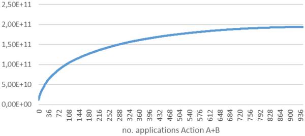
Figure 10 SHA-3 cycle length after repeated Action A and B application.

It can be seen, that the cycle length increase with a factor of 16.6 after 943 actions is still significant, which shows that the breakout method is also useful to improve the cycle length of SHA-3. The figure furthermore shows that for a repeated application of Action A and B, the average cycle length increase also becomes smaller for an increasing number of iterations. It runs into a saturation, similar to the behavior for Action A only. This can be explained by the fact that the algorithm that choses the components to be merged during Action B based on the size of the component, so the merged components get smaller for each application. At the same time, the gain of the Actions A that follow an Action B becomes smaller accordingly.

In order to evaluate the potential positive or negative impact of the break-out method to the statistical properties of the PRNGs, the original and modified versions of the algorithms have been analyzed with the NIST statistical test suite. The NIST suite has been chosen, because it covers a wide range of different tests and is easily applicable on a larger number of input values.

Figure 11 depicts the percentage of passed NIST tests for the 100 sequences of the shortened version of MD5 that have been analyzed. The results are simply ordered by percentage to allow an easy overview. The blue dashed line is the result for the unmodified function and the grey dotted line for the breakout using Actions A and B.

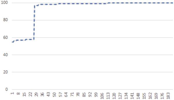
Figure 11 Passed NIST Tests for MD5.

Figure 12 shows the same data for the 1000 sequences of the shortened version of SHA-3. It can clearly be seen that there is only a negligible difference between the original and the versions modified using Actions A and B. The dashed and the dotted lines are congruent, as the same p-values are calculated for both versions. This shows that the statistical properties of the PRNGs are not negatively impacted by the application of the breakout mechanism.

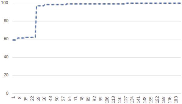
Figure 12 Passed NIST Tests for SHA-3.

6 Conclusion

We have presented a parallel algorithm for finding promising candidate states to modify the state transition function of a pseudo-random number generator. Use of these candidates allows to increase the cycle length notably, which is helpful if the state space itself cannot be enlarged due to resource constraints such as performance and energy in embedded devices. The inherent load balancing problems of this algorithm can be resolved by the use of an ant colony-like strategy: paths that are not followed further because of meeting another path donate their time to the other path that can then progress faster. This illustrates once more how nature can inspire improvements in security-related algorithms. The resulting parallel algorithm exhibits regular structure and high efficiency even for large thread count, and thus is suited for massively parallel computing engines like GPUs.

As future work, we would like to extend our work towards similar primitives such as stream ciphers. Here, Spritz [16] might be a good candidate, as it would also allow to extend our work from non-bijective towards bijective transition functions.

Acknowledgement

We thank Christoph Kessler of Linköpings Universitet in Sweden for his help modeling the exploration of unknown trees and the distinction of the online and oﬄine case.

References

[1] Andreas Beckmann, Jaroslaw Fedorowicz, Jörg Keller, and Ulrich Meyer. A structural analysis of the A5/1 state transition graph. In Proc. First Workshop on GRAPH Inspection and Traversal Engineering, volume 99 of Electronic Proceedings in Theoretical Computer Science, pages 5–19. Open Publishing Association, 2012.

[2] Alex Biryukov, Adi Shamir, and David Wagner. Real time cryptanalysis of A5/1 on a PC. In Fast Software Encryption, pages 37–44. Springer, 2001.

[3] Anand Desai, Alejandro Hevia, and Yiqun Lisa Yin. A practice-oriented treatment of pseudorandom number generators. In International Conference on the Theory and Applications of Cryptographic Techniques, pages 368–383. Springer, 2002.

[4] Yevgeniy Dodis, David Pointcheval, Sylvain Ruhault, Damien Vergniaud, and Daniel Wichs. Security analysis of pseudo-random number generators with input:/dev/random is not robust. In Proceedings of the 2013 ACM SIGSAC Conference on Computer & Communications Security, pages 647–658. ACM, 2013.

[5] Marco Dorigo and Luca Maria Gambardella. Ant colony system: a cooperative learning approach to the traveling salesman problem. IEEE Transactions on evolutionary computation, 1(1):53–66, 1997.

[6] Philippe Flajolet and Andrew M. Odlyzko. Random mapping statistics. In Advances in Cryptology, pages 329–354. Springer, 1990.

[7] Jovan Golic. Cryptanalysis of alleged A5 stream cipher. In Walter Fumy, editor, Advances in Cryptology (EUROCRYPT ’97), volume 1233 of Lecture Notes in Computer Science, pages 239–255. Springer Berlin Heidelberg, 1997.

[8] Jan Heichler, Jörg Keller, and Jop F. Sibeyn. Parallel storage allocation for intermediate results during exploration of random mappings. In Proc. 20th Workshop Parallel-Algorithmen, -Rechnerstrukturen und -Systemsoftware (PARS ’05), pages 126–134. GI, June 2005.

[9] Jörg Keller. Parallel exploration of the structure of random functions. In Proceedings of the 6th Workshop on Parallel Systems and Algorithms (PASA) in conjunction with the International Conference on Architecture of Computing Systems, ARCS, pages 233–236. VDE, 2002.

[10] Jörg Keller, Gabriele Spenger, and Steffen Wendzel. Ant colony-inspired parallel algorithm to improve cryptographic pseudo random number generators. In Proc. BioSTAR/IEEE Security & Privacy Workshops, May 2017.

[11] Donald E. Knuth. Mathematical analysis of algorithms. In Proc. of IFIP Congress 1971, Information Processing 71, pages 19–27. North-Holland Publ. Co., 1972.

[12] Leslie Lamport. Password authentication with insecure communication. Commun. ACM, 24(11):770–772, November 1981.

[13] George Marsaglia. The marsaglia random number cdrom including the diehard battery of tests of randomness, 1995.

[14] Honorio Martin, Enrique San Millan, Luis Entrena, Pedro Peris Lopez, and Julio Cesar Hernandez Castro. AKARI-X: A pseudorandom number generator for secure lightweight systems. 11th IEEE International On-Line Testing Symposium, pages 228–233, 2011.

[15] Alfred J. Menezes, Paul C. van Oorschot, and Scott A. Vanstone. Handbook of Applied Cryptography. CRC Press, 1996.

[16] Ronald L. Rivest and Jacob C. N. Schuldt. Spritz—a spongy RC4-like stream cipher and hash function. Cryptology ePrint Archive, Report 2016/856, 2016. http://eprint.iacr.org/2016/856.

[17] Andrew Rukhin, Juan Soto, James Nechvatal, Miles Smid, and Elaine Barker. Statistical test suite for random and pseudorandom number generators for cryptographic applications: Special publication 800-22, revision 1a, 2010.

[18] Gabriele Spenger and Jörg Keller. Tweaking cryptographic primitives with moderate state space by direct manipulation. In Proc. IEEE International Conference on Communications (ICC’17), pages 1–7. IEEE, May 2017.

Biographies

images

Jörg Keller is a professor of computer engineering at FernUniversität in Hagen, Germany, and heads the Parallelism & VLSI group since 1996. His research interests are parallel and energy-efficient computing, security and fault-tolerance of computer systems, and web-based learning in engineering. He received M.Sc. and Ph.D. degrees from Saarland University, Germany, in 1989 and 1992, respectively, and spent his PostDoc phase at CWI (Netherland’s Research Centre for Mathematics and Computer Science) in Amsterdam.

images

Gabriele Spenger is a Ph.D. student at the Parallelism & VLSI group of FernUniversität in Hagen, Germany. Her research focus is on security and RFID. She received her diploma in Mathematics from Friedrich-Alexander-Universität, Germany in 1998.

images

Steffen Wendzel received his Ph.D. degree in computer science from the University of Hagen in 2013, Germany. Between 2013 and 2016, he was head of a smart building security research team at Fraunhofer FKIE, Germany. He joined Worms University of Applied Sciences as a professor of information security and computer networks in 2016. Steffen wrote five books and his research focuses on information hiding and security in the Internet of Things.