Biometric Authentication Using Mouse and Eye Movement Data

Jamison Rose¹, Yudong Liu² and Ahmed Awad³

¹Versive
²Computer Science Department, Western Washington University, Bellingham, WA, USA
³School of Engineering & Computing Sciences, New York Institute of Technology, Vancouver, Canada

E-mail: jamison@jamisonrose.com; yudong.liu@wwu.edu; Ahmed.Awad@nyit.edu

Abstract

Previous biometric systems have attempted to identify users solely by eye or mouse data. In this paper, we seek to find out if combining both kinds of data produces better results. In our system, mouse movement and eye movement data are gathered from each user simultaneously, a set of salient features are proposed, and a Neural Network classifier is trained on this data to uniquely identify users. After going through this process and investigating several Neural Network based classification models we conclude that combining the modalities results in a more accurate authentication decision and will become practical once the hardware is more widespread.

Keywords

Biometric Authentication
Mouse Movement
Eye Movement
Neural Network Classifiers

1 Introduction

Biometrics is the study of methods that uniquely identifies individuals based on their traits. There are two subsets of biometrics, physiological and behavioral [4]. Physiological methods include fingerprint scanning, iris scans, hand geometry recognition or facial recognition, all of which involve measuring physical characteristics of a person [4]. They are useful because they do not change much for a user over time. One downside of physiological biometrics is that if the biometric template is ever obtained and the user is compromised the system cannot be updated without body modification. Physiological biometrics are usually used for a static verification that a user does once, and as such, leaves the computing session susceptible to attack afterwards. Behavioral biometrics are unique to a person in how they act or think. Studies in this field include keystroke dynamics [3, 12, 17, 20], mouse dynamics [1, 16, 23, 24, 28], voice recognition [7, 32], signature verification [4, 18, 34], Graphical User Interface (GUI) pattern analysis [2] and touchscreen feature analysis [9, 33]. Behavioral biometrics can not only be used for static verification at the beginning of a user’s session, but can also be used dynamically to continuously authorize a user during a session. Behavioral templates cannot be obtained as easily as physiological ones given that authentication can take place dynamically throughout a user’s session as opposed to occur once statically; so compromising a user should be more difficult. These biometrics are susceptible to errors due to users gaining experience, changing the way they act with a system.

Most of the traditional biometric systems are unimodal systems, where a single biometric trait of the individual is used for identification. Multimodal systems [11, 27, 30, 31], unlike unimodal ones, take input from single or multiple sensors for measuring two or more different biometric characteristics. In addition to improving the identification accuracy, combining two or more biometric modalities might be more appropriate for different applications. An examples of multimodal systems would be a biometric system that combines fingerprint, face, and speech [15].

In this paper, we will report our work of combining mouse dynamics and eye movement data in user authentication. Most previous research has been focused on one of these dynamics or the other but little to none exist that combine them. [6], however, suggests that eye movement and mouse movement have an 84–88% correlation. Because of this strong correlation we believe that training a system on data from both sources will provide better results when compared to systems that only use data from one source. In this paper we will describe a system by which to gather both kinds of data from users and create a system that can authorize them. The system will need to do data preprocessing in order to clean the data, split it into meaningful segments, and provide datasets for both training and testing. We will then extract features from the data for use in a Neural Network classifier in order to identify individual users. Finally we will evaluate the system experimentally and discuss obtained.

The rest of the paper is structured as follows. Section 2 provides background information on biometric system performance and discuss related work. Section 3 introduces our experimental setup. Section 4 describes the features we used for the system. Section 5 introduces our Neural Network based machine learning system. In Section 6 we will report the experimental results and discuss on the results. We conclude our work in Section 7.

2 Biometric System Evaluation Metrics and Related Work

While understanding how previous systems work is important, it is also important to know how to evaluate a biometric system. Most research in this field uses False Acceptance Rate (FAR) and False Rejection Rate (FRR) or equivalent measures to evaluate the performance of a system. In order to calculate these metrics, recognition systems have to be tested by both attacking the system with legitimate users that should be accepted and illegitimate users that should be rejected. Users attacking themselves should be accepted resulting in true positives. If they are not accepted this is a false negative. Users attacking other users should be rejected forming true negatives. If they are accepted this is a false positive. FAR is calculated by dividing the total number of false positives by the total number of attacks that should have been negative (false positive plus true negatives). The FRR is calculated by dividing the number of false negatives by the total number of things that should be labeled positive (true positives plus false negatives). These metrics are more useful than a normal accuracy measurement because they give a more complete picture of what a system can achieve. In addition, system performance is often reported in terms of Equal Error Rate (EER), which is the operating point at which FAR = FRR.

2.1 Mouse Tracking

Data for mouse dynamics comes from features extracted from how a user moves a mouse which is typically gathered while they naturally use a computer or do a controlled task. [28] provides a detailed description of biometrics in the context of mouse dynamics. Much of this work was modeled after one of the pioneering works in the field by [1]. In their work they gathered data by having users move their mouse in one of eight directions to form an action and recorded many of these actions per user. They then identified patterns in these actions that fell into several categories. Depending on the distribution of these categories during an action and based on several features such as speed, distance, and direction they were able to train a system to have an FAR and FRR of about 2.4%. Another related work [35] suggested using the interior angle of a sliding window of points might describe the curvature of an action well and by extracting this feature and several others were able to train a support vector machine (SVM) to an FAR and FRR of 1.3%. We borrowed ideas from both of these works when extracting features for our own. Other studies focused on the viability of mouse dynamics in a continuous authentication setting. [29] proposed that many methods may not be sufficient to be used continuous identity authentication and monitoring, such as online monitoring. They focused on extracting features in a way that would be best in such an environment, and were able to achieve an FAR of 1.86% and FRR of 3.46% using SVM (Support Vector Machine). Many papers emphasized the trade-off between time taken to authenticate and accuracy of the system involved. [29] also showed that a low number of samples (corresponding to a low sample time) provided worse results than that of a large sample size system. They showed the relation of FAR and FRR in session times from less than a second to about twenty minutes. At authentication times under a second they had an FAR of 33% and FRR of 38%. At times around twenty minutes they were able to achieve 0.1% FAR and 0.0% FRR.

2.2 Eye Tracking

More recently research has been done on the use of eye movement dynamics for biometric authentication [5, 19, 25, 26]. Eye movement dynamics are similar to mouse dynamics except they track eye movement on a screen rather than the mouse. They are less practical to gather for average users because of the requirement of specialized and sometimes expensive hardware. In a study of various eye trackers [14] it was found that a temporal resolution of 250 Hz is recommended for biometrics and anything under 30 Hz will probably not produce data with enough quality to be viable. [8] explored what type of stimuli would provide the best results for biometrics. They found that images that required tracing a path created some of the best dynamics. [10] reported a biometric system that uses eye movement tracking and was able to achieve a performance of an FAR of 21.45% and an FRR of 47.2%. To achieve this they trained a system by extracting features for eye velocity, eye movement direction, and distance traveled. [13] was able to achieve an FAR and FRR of 27%. To reach this accuracy they used data gathered from users reading text. While extracting features they focused on the traits of the data that are typically more unique to eye tracking data which included features that contained information on the fixation points and features that had information on the saccades a user’s eyes made while reading.

3 Experimental Setup

3.1 Data Gathering

3.1.1 Hardware configuration

Our system involved using eye tracking and mouse movement data to predict user identity. The mouse we used was a Razor Ouroboros¹ gaming mouse that was configured to have a sampling rate of 1000 Hz. The eye-tracker we used to gather data was a SensoMotoric Instruments (SMI) iView RED-m² and had a sampling rate of 120 Hz. We used a desktop computer running Windows 8 with a screen resolution of 1680 by 1050 pixels on a 23 inch monitor.

3.1.2 Participants

Participation in the study was entirely voluntary and anyone who wanted to take part in the study was allowed given the eye tracker was able to calibrate to their eyes. The users were calibrated based on a five point calibration system and were repeatedly calibrated until they could reach a spatial accuracy of at worst 0.5. Users that could not achieve this accuracy were not included in the data set. Of the forty-two participants that volunteered thirty-six were male and six were female. Ten users, eight male and two female, were unable to calibrate well due to the limitation of the hardware and most of these participants wore glasses. This leaves thirty-two users tested, twenty-eight male and four female. The users age ranged from eighteen to forty-seven with an average age of twenty-five. The average number of years a participant had using a computer was eighteen. Fifteen of the users did not require any form of corrective lenses to see while the other seventeen did.

3.1.3 Experiment procedure

To gather data for the evaluation of our system we asked for volunteers to take part in a simple activity during which we could record their data. During the experiment each user was asked to click a series of buttons in order. Our interface included a button in the center of the screen and eight buttons spread around the edges of the screen in a circle. See Figure 1 for the layout of the interface. The user would perform an action by clicking the center button and then clicking on one of the buttons on the outer edge. The button the user needed to click next was highlighted in a bright green color. Each sample within an action included a timestamp measured in nanoseconds and the position of the eyes or mouse represented as a horizontal and vertical coordinate in pixels on the screen. Each user was asked to perform at least twenty-four of these actions in each direction so that we would have enough data to evaluate the system later on. Altogether each user generated a minimum of one-hundred and ninety-two of these samples. This data was split into two datasets each containing half of the data. Each data set had an equal amount of data in each direction the user performed an action. One was used for training and one for testing the trained system. While testing the system we found that the eye tracker sometimes lost track of the users eyes causing it to create noise samples that were of little use to us. To counteract this we built checks into the system to ensure that a user was able to generate enough clean samples to meet the requirements. We had them generate additional samples until they had enough.

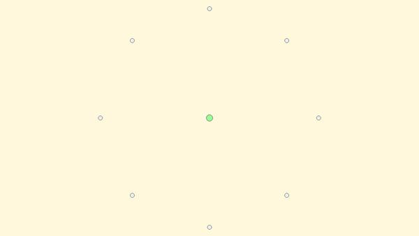
Figure 1 User interface for user data gathering.

3.2 Data Observations

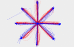
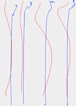
Once all user’s data was gathered each dataset was visualized. In Figure 2 a sample user’s data can be seen. The blue lines represent the eyes movement and the red lines represent the mouse movement. The lines drawn are formed by doing a linear interpolation between data points. Most user’s data looks fairly similar with a cursory glance, but there are differences between different users especially in the shape of their paths. Most users have a straight path in both the vertical and horizontal movements, but a curved path in each of the diagonal directions. This applies to both the eye movements and the mouse movements. The degree to which the path curves, how tightly it curves, and whether it curves up or down were unique to each user; more so when taking into account all directions. Sometimes two users had similar looking paths in one direction, but none of them had similar looking paths in all directions. Two important observations are that although the eye and mouse lines correlate well with each other they have significant distance between them (See Figure 3 for a closeup of the distance between the eye movement and the mouse movement in one sample direction for a random user) and that users have more data points near the beginning and end of their actions for both the eye and mouse movement lines. These clusters of data are called fixation points because the users focus is fixated in a small area for a duration of time. Due to these observations we split the data into three subsets. More information on this process is in Section 3.3.2.

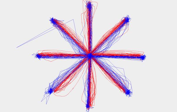
Figure 2 Sample user data. The blue lines represent the eyes movement and the red lines represent the mouse movement.

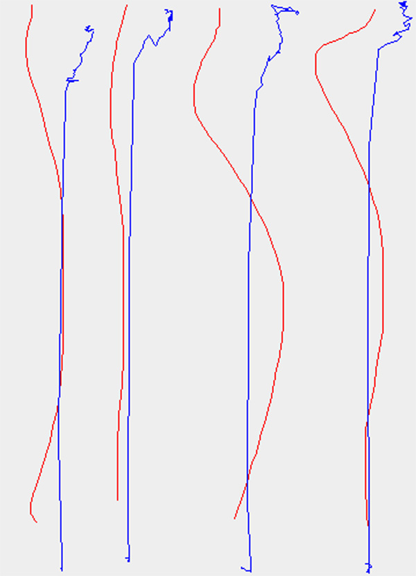
Figure 3 A closeup of the distance between the eye movement path and the mouse movement path in one sample direction for a random user.

3.3 Data Preprocessing

During our exploratory work in the research we found that cleaning too aggressively can lead to there not being enough data to train the system properly. Because of this we tried to clean as minimally as possible and use data that might otherwise be cleaned in other ways. Originally we removed much of the fixation data of the mouse and eyes, but this left little data for some users so instead we used a data splitting process to keep it.

3.3.1 Data cleaning

The only data removed from the actions before further preprocessing and feature extraction were data points that fell off the screen or corresponded to the user blinking which was shown in the data as the user looking at the point (0, 0) on the screen. If this process leads to the action having less than ten data points then the action was discarded and not used in our dataset. This process did not reduce the total amount of data in a significant way.

3.3.2 Data splitting

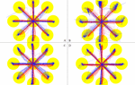
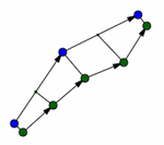
During the data splitting process each sample was split into three regions. One region each for the start and end points and a third region that included all other data. The area around the start and end points was defined using a radius that could be tuned. Figure 4 shows four different user’s data. The yellow circles show the regions around the start and end points that are separated into their own sets of features. The radius appears large, but this is mostly because different users fixations skewed in different directions from the end points. This can be seen by comparing users A and B in Figure 4. User A has very small fixation points so a smaller radius would make more sense for them, but user B does not fixate on one point as much as can be seen in their vertical direction. These two users are close to the extremes of user fixation distribution. Most users fall somewhere between these two. User C illustrates how sometimes a user can have small fixations in most directions, but more spread fixations in others. Their vertical and horizontal fixations are fairly tight and the diagonals less so; especially in the lower right corner. User D shows how some users have fairly tight fixations with few outlier fixations where they were less focused. This process is helpful because the data that occurs during the fixation periods of a user’s actions are significantly different from the data created during the other times. Speed, separation, and change in orientation all are different during fixation. So if the averages of these were used as features they would be biased towards the data of intense fixations and the in-between actions would be less significant. Other than removing some bias this method also increases the amount of features that can be generated for a classifier such as a neural network to learn from which improves the system. But it comes with its own drawbacks. More features provide a better description to the neural net which allows it to train while converging to a lower error, but three times as many features causes it to train much more slowly. Overall training to a lower error rate was valued more than the time loss so we implemented the splitting technique and tried to use other methods to speed up the process.

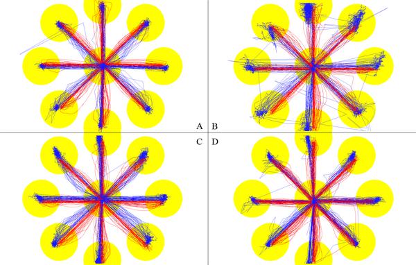
Figure 4 Data splitting diagram for four different users.

3.3.3 Data normalization

To help counteract some of the time loss from the Data Splitting process, the data was normalized before being used by the neural networks. To achieve this the mean and standard deviation of the training data was found and used to remap the data to occur between –1 and 1 while maintaining the same distribution centered at 0. The testing data was similarly altered using the same mean and standard deviation that were computed from the training set.

4 Features

After preprocessing the data we needed to extract features from it to feed our neural network. The features we included were the average speed of the eye, the average speed of the mouse, the average angle of deviation from vertical of the eye, the average angle of deviation from vertical of the mouse, the average interior angle of the eye, the average interior angle of the mouse, and the average separation of the eyes and mouse. More detailed explanations of these features are as follows:

4.1 Speed

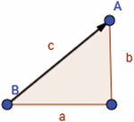
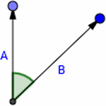
It is defined as the average speed ( $\bar{v}$ ) of the eyes was found by dividing the distance (c) traveled between two points by the time (t) taken to travel between those two points.

c = \sqrt{a^{2} + b^{2}} (1)

In Figure 5 this calculation would be done between points A and B. Lengths a and b are measured and used to calculate length c which is then used in the velocity equation.

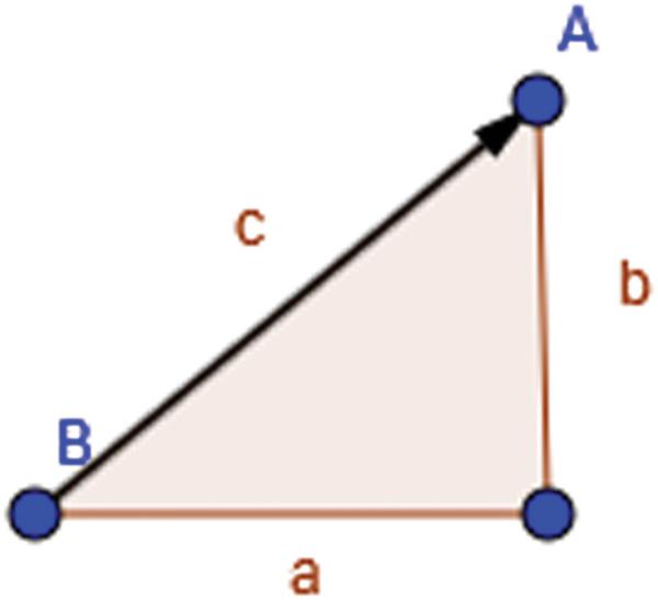
Figure 5 Distance calculation.

v = \frac{c}{t} (2)

These values were then summed across all consecutive pairs of points and divided by the total number of points (n) to get the average.

\bar{v} = \frac{1}{n} \sum_{1}^{n} v_{i} (3)

This calculation was used for both eyes and mouse points.

4.2 Vertical Angle

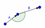
The average angle of deviation from vertical for each sample is useful because it describes how far off from a straight line the user made while creating a sample (See Figure 6). The angle (α) was found by creating two vectors and finding the angle between them.

Figure 6 Vertical angle calculation.

α = \arccos (\frac{A \cdot B}{| A | | B |}) (4)

The first vector was between two consecutive points in a sample and the second was a unit vector directly vertical from the first point in the pair.

4.3 Interior Angle

The interior angle is similar to the Vertical Angle, but with these other vectors instead (See Figure 7). This angle is useful because it describes how tightly a user turns when adjusting the path of their eyes or mouse.

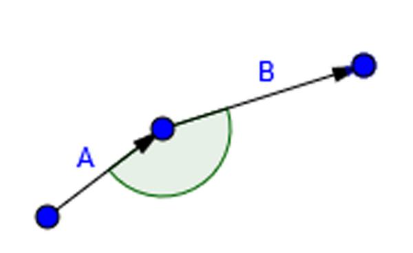
Figure 7 Interior angle calculation.

4.4 Separation Calculation

The separation calculation measures the distance between the eyes and the mouse at any given time (See Figure 8). The eyes and mouse were sampled at different rates which caused there to be many more mouse samples than eye samples. To account for this the separation was measured between each mouse point and the corresponding point on the eye path. To find the corresponding point on the eye path two points were found on it that were on either side of the mouse point with respect to time. These two points were then linearly interpolated based on the time of the mouse point. For example if the mouse point occurred at time 10 and samples for the eyes only existed at times 0 and 20 then these two points would be linearly interpolated and the point halfway between them would be selected. Then the same distance formula as used in the speed feature can be used to compute the distance.

Figure 8 Separation calculation that measures the distance between the eye path and the mouse path at any given times.

5 Machine Learning System

Once feature extraction was complete we had to create a machine learning system. The library we used to train our system was the Accord. Neuro³ C# library. All instances of neural networks were trained using Bipolar Sigmoid as the activation function which means it does best when the output is a number between –1 and 1. These neural networks used the Nguyen Widrow [22] method for random initialization and Levenberg Marquardt [21] backpropagation for training. For each user a separate neural network was created that tried to answer the question “Does the input user data belong to the trained user?”.

5.1 Network Input

The data that was input into the system came directly from the features that were extracted. The network for each user was trained on their own data as positive examples and on all other user’s data as negative examples. The network was trained so that it should produce a result that can be interpreted as meaning to accept or reject a user based on whether the data was a positive example or negative example. Since there were more negative examples than positive examples for the network to train on we tried limiting the number of negative examples to be a multiple of the users positive examples. To select which samples would be used in the limited case we randomly selected an evenly distributed number of samples from each negative user so that they were evenly distributed across each direction. We sampled data in this manner because we wanted the network to have a wide range of knowledge about other users. This process does two things for the system. First it should make the system less biased towards rejecting a user and second it limits the amount of data that the system has to train on from a factor of n², assuming each user has a similar amount of data, to a factor of kn where n is the number of users and k is the multiple of n used when reducing the amount of negative examples. Even though this drastically reduces the training time of the entire system, the results of this were significantly worse than when all negative examples were used in training during all of our test cases. Thus this method was not used in the final system.

5.2 Network Structure

The networks tested included those with a single input layer, one to two hidden layers, and a single output layer. The input layer for most networks had twenty-nine input nodes. Twenty-one nodes corresponded to the speed, vertical angle, interior angle (these 3 types of features are extracted from the eye movement data and mouse movement data, respectively), and separation features, each of which was split into the three different zones; The remaining eight were used to encode the direction (as shown in Figure 4, we have 8 different directions in which the eyes and the mouse can move) using one-hot encoding. Networks were also tested without data splitting causing the input vector to be fifteen input nodes. The networks without data splitting performed worse in every test compare to their split counterparts so they were not pursued extensively. Finally networks that only used eye or only used mouse data were trained with seventeen input nodes. These networks only trained on speed and angles of one form of data or the other. Separation was left out of these since it depends on both. The hidden nodes were tested in configurations ranging from the number of input layer plus one up until one-hundred nodes each. The output node returned a value between –1 and 1 corresponding to how confident the network was that a user was who they said they were.

5.3 Network Output

While training each network the output for feature vectors that belonged to the currently trained genuine user were marked with a 1 and samples that did not belong to the current user were marked with a –1. A confidence value was calculated by running an action through the trained network for a user. One to four actions in each direction were batched into a session and each was evaluated by the system. All output confidence values in a session were then averaged to get the overall confidence of a session. This allowed the data unique to each direction to contribute to the overall confidence. To interpret the results a threshold was chosen for each user that would accept an input if the output confidence value for a session was greater than the threshold and reject otherwise. The threshold also required tuning for the final system. To tune the threshold, values were chosen that maximized the resulting F-score and values were also chosen that made the distance between FAR and FRR the smallest. In statistical analysis of binary classification, the F-score (also F-measure) is a measure of a test’s accuracy. F-score ranges from the worst value of 0 to the best value of 1. The threshold with the minimum distance between FAR and FRR is the point of Equal Error Rate (EER). Maximizing F-score and minimizing EER typically gave slightly different scores so both are recorded in the results.

6 Results and Discussion

6.1 Tuning Parameters

To tune the system it was trained on the training data set using the a set of tuning parameter values and then tested on the testing set to see how the system performed with that set of tuning parameters values. This was done many times to find the optimal configuration of tuning parameters. Altogether there were three tuning parameters that were varied while testing the system. First the split radius during the data splitting process was varied. While tuning the value, we found the value that gave the best results was around 180 ± 25 pixels. This appeared to be about the size the radius needed to be to encompass all of the data in the end points for some of the users that had looser fixations. Next we varied the layer structure of the neural networks. We tried networks with one to two hidden layers and up to one-hundred nodes in each layer. The networks for both the combined and separated data sets performed best when there was about forty-three nodes in the hidden layer and additional layers. Finally, the confidence threshold was trained by testing thresholds in the range of all output confidence values while testing the system. This was necessary to generate the ROC curves explained in Section 6.3.

6.2 Eye and Mouse Results

The results for testing the system by using both eye and mouse data can be seen in Table 1. Each system was tested using a batch size of four samples in each direction or thirty-two samples overall. Both the five user and fifteen user system were able to train to very low error rates. When evaluating the systems they were able to perfectly guess the training dataset, but results are reported by evaluating the system with the testing data set.

Table 1 The results of combining eye and mouse data on 5, 15 and 32 users when maximizing F-score and minimizing EER

		F-Score Max (%)			Min EER (%)
Num of Users	Neural Network Structure	F-Score	FAR	FRR	F-Score	FAR	FRR
5	29-30-1	93.3	5.0	0.0	93.3	5.0	0.0
15	29-43-43-1	67.6	22.4	0.0	64.6	12.9	5.2
32	29-43-43-1	37.8	52.9	0.0	35.1	13.3	43.8

6.2.1 5 Users

While training the system on only five users the system was able to achieve 5% FAR and 0% FRR. The users were chosen at random from the 32 users we gathered data from. This result was found by splitting the data with a 200 pixel radius and a neural network that had a single hidden layer with thirty nodes.

6.2.2 15 Users

A system trained on fifteen users was able to achieve 12.9% FAR and 5.2% FRR. These fifteen users were the fifteen users that had the best calibration with the eye tracking system. For this setup the data was split with a 180 pixel radius and a neural network that had two hidden layers, each with forty-three nodes.

6.2.3 32 Users

The system trained on thirty-two users incorporated all users that we gathered data for. It was able to achieve an FAR of 13.3% and an FRR of 43.8%. It was trained with data that was split on a 180 pixel radius and a neural network with two hidden layers each with forty-three nodes.

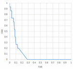
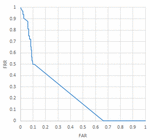
6.3 System Evaluation

Once our systems were trained each one needed to be tested to find its optimal FAR and FRR value. When graphed together with respect to one another they form the Receiver Operating Characteristic (ROC) curve. Figures 9, 10, and 11 show the ROC curves generated to show the relation of the FAR and FRR when the confidence threshold to accept a user is varied. The relation between FAR and FRR in a ROC curve is useful because not all system implementations have the same definition of “best” in terms of system performance with respect to FAR and FRR. Sometimes certain thresholds have to be met while others can be sacrificed. For example in the case of fifteen users if a system required less then 10% FAR the curve shows that the best FRR achievable would then be around 40%. Several dozen configurations of the system were trained in order to find the best tuning parameters. Once the best tuning parameters were determined the best performing system for each test was trained at least twice to check for consistency. In all consistency checks the system was able to train within about 1% difference in FAR and FRR values. Only the best trained system for each type is reported in the results.

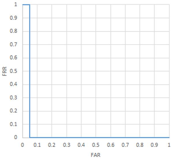
Figure 9 ROC curve (5 Users).

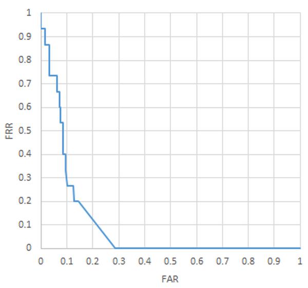
Figure 10 ROC curve (15 Users).

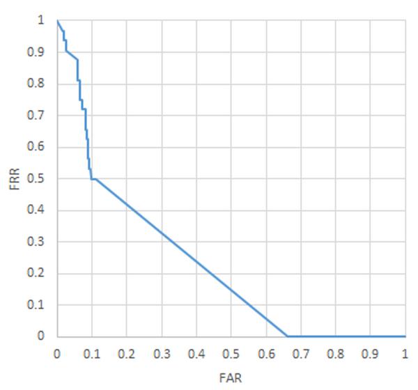
Figure 11 ROC curve (32 Users).

6.4 Mouse Only and Eye Only Results

Table 2 shows a comparison of the mouse only and eye only systems trained for comparison. All systems were evaluated with a batch size of four samples in each direction. All systems took considerably longer than the combined system to train by a factor of roughly ten. While training the split system also converged to points with higher error rates than that of the combined system, as the table shows uncombined data performed worse in all but one case. When tested with five user’s data, the eye data only trained system was able to perform as well as the combined system, but not better. Overall the combined data performed much better than the separated data.

Table 2 The results of Eye-only and Mouse-only data on 5, 15 and 32 users when Maximizing F-score and Minimizing EER

			F-Score Max (%)			Min EER (%)
Type	Num of Users	Neural Network Structure	F-Score	FAR	FRR	F-Score	FAR	FRR
Mouse Only	5	17-45-1	80	25.0	0.0	73.3	10.0	20.0
	15	17-45-45-1	55	42.4	0.0	50	11.9	40.0
	32	17-43-43-1	17.9	79.0	0.0	14.2	23.9	59.4
Eyes Only	5	17-40-1	93.3	5.0	0.0	93.3	5.0	0.0
	15	17-43-1	43.6	51.4	0.0	38.6	17.1	40.0
	32	17-45-1	23.4	64.6	0.0	19.9	14.0	56.3

6.5 Cross Validation

Due to having a limited amount of data a development set was not used during the process of tuning. Instead a training and testing set was generated based on a fifty–fifty split of the available data. The system was trained on the training set and evaluated on the testing set. In order to show that this did not bias the system we also generated five additional training and testing sets by randomly splitting the data each time. In each case the specific users included were the same, but the data in each set was different. We then trained and tested these additional data sets to see what effect optimizing on a specific set had. See Table 3 for the results of this cross validation. Note that amounts given in this table are averages across the five cross validation trials.

Table 3 The results of cross validation on the combined data set

		F-Score Max (%)			Min EER (%)
Num of Users	Neural Network Structure	F-Score	FAR	FRR	F-Score	FAR	FRR
5	29-30-1	79.4	22.8	0.0	75.3	19.2	0.12
15	29-43-43-1	52.8	40.5	0.0	48.4	18.9	34.6
32	29-43-43-1	24.5	65.72	0.0	20.9	19.2	56.2

7 Conclusion and Future Work

Overall the method used to train the system seems to work well for a small number of users, but does not scale well as the number of users increases. We believe that this is because as the number of users increases the amount of negative training examples increases which gives the system a bias. Decreasing the amount of negative examples did not work as a method to fix this because the system tries to determine a user from a pool of users and reducing the number of negative examples provides a less complete picture to the system of that pool. To overcome this limitation the system would need to either increase the number or complexity of the features, or be trained in such a way that the system only needed positive examples.

As the results show the system performed far better when the two data types were trained together. They show that even for a somewhat weak system such as ours it boosts performance by a great deal. Not only did they improve the quality of the system, but they allowed training to occur faster. The training algorithm for the data combined usually took about an hour to train on an average single user desktop whereas the two separated data sets took anywhere from six to twelve hours to converge. Even when the separated data sets did converge they converged at error rates that were much higher than those of the combined system. Overall we observed that this pattern existed in all tests we performed and we believe it will hold true for more complex systems in the future. Assuming that the hardware for the system is readily available we would recommend pursuing combining metrics like the ones presented in this paper.

In the future there are a number of other paths we would like to follow to try for better results. Training a system that identifies eye and mouse behavior such as saccades and fixations should be able to achieve a better FAR and FRR when the data is compared through alignment and the relevant features are extracted. Our current work was more a proof of concept. That is the core question we were trying to answer is if combining the data sources had merit. The complexity of the features we extracted provided far less information than that of other contemporary work. This provided simplicity in the design and implementation, but definitely impacted performance. The main reason the data sources would not have had merit would be if they were too cross correlated to provide unique information and in that case the score would not have improved when we used the data together. A feature analysis would help us identify the important features as well as redundant ones. A richer feature set suggested by previous work on authentication using mouse dynamics could also be used in our system. More sophisticated Neural Networks such as Recurrent Neural Networks (RNNs) and Long Short Term Memory Networks (LSTMs) could also be used for what we’re dealing with is essentially time series data. By improving the strength of the system we will be able to tell if the improvement from incorporating eye and mouse data scales with system strength or if it is a constant gain. Other than improving the quality of our features we would like to explore systems that train on user data gathered through composite movements rather than movements in a single direction. Finally to get the better results we need to gather data from users using an eye-tracking system with a temporal resolution of at least 250 Hz.

References

[1] Ahmed, A., and Issa, T. (2007). A new biometric technology based on mouse dynamics. IEEE Trans. Dependable Sec. Comput. 4, 165–179.

[2] Bailey, K. O., Okolica, J. S., and Peterson, G. L. (2014). User identification and authentication using multi-modal behavioral biometrics. Comput. Sec. 43, 77–89.

[3] Bergadano, F., Gunetti, D., and Picardi, C. (2002). User authentication through keystroke dynamics. ACM Trans. Inform. Syst. Sec. 5, 367–397.

[4] Bhattacharyya, D., Ranjan, R., Alisherov, F., and Minkyu, C. (2009). Biometric authentication: a review. Int. J. Serv. Sci. Technol. 2, 13–28.

[5] Cantoni, V., Galdi, C., Nappi, M., Porta, M., and Riccio, D. (2015). Gant: gaze analysis technique for human identification. Pattern Recogn. 48, 1027–1038.

[6] Chen, M. C., Anderson, J. R., and Sohn, M. H. (2001). “What can a mouse cursor tell us more?: correlation of eye/mouse movements on web browsing,” in Proceedings of the CHI ’01 Extended Abstracts on Human Factors in Computing Systems, CHI EA ’01 (New York, NY: ACM), 281–282.

[7] Chetty, G., and Wagner, M. (2006). “Multi-level liveness verification for face-voice biometric authentication,” in Proceedings of the Biometric Consortium Conference, 2006 Biometrics Symposium: Special Session on Research (Rome: IEEE), 1–6.

[8] Darwish, A., and Pasquier, M. (2013). “Biometric identification using the dynamic features of the eyes,” in Proceedings of the IEEE Sixth International Conference: Biometrics: Theory, Applications and Systems (BTAS), Arlington, VA, 1–6.

[9] De Luca, A., Hang, A., Brudy, F., Lindner, C., and Hussmann, H. (2012). “Touch me once and i know it’s you!: implicit authentication based on touch screen patterns,” in Proceedings of the SIGCHI Conference on Human Factors in Computing Systems (New York City, NY: ACM), 987–996.

[10] Dhingra, A., Kumar, A., Hanmandlu, M., and Panigrahi, B. K. (2013). “Biometric based personal authentication using eye movement tracking,” in Proceedings of the 4th International Conference on Swarm, Evolutionary, and Memetic Computing – Volume 8298, SEMCCO 2013 (New York, NY: Springer-Verlag New York, Inc), 248–256.

[11] Fierrez-Aguilar, J., Ortega-Garcia, J., Gonzalez-Rodriguez, J., and Bigun, J. (2005). Discriminative multimodal biometric authentication based on quality measures. Pattern Recogn. 38, 777–779.

[12] Giot, R., El-Abed, M., and Rosenberger, C. (2009). “Keystroke dynamics authentication for collaborative systems,” in Proceedings of the CTS’09 International Symposium: Collaborative Technologies and Systems, 2009 (Rome: IEEE), 172–179.

[13] Holland, C., and Komogortsev, O. V. (2011). “Biometric identification via eye movement scanpaths in reading,” in Proceedings of the 2011 International Joint Conference: Biometrics (IJCB), San Jose, CA, 1–8.

[14] Holland, C. D., and Komogortsev, O. V. (2012). “Biometric verification via complex eye movements: the effects of environment and stimulus,” in Proceedings of the 2012 IEEE Fifth International Conference: Biometrics: Theory, Applications and Systems (BTAS), Montreal, QC, 39–46.

[15] Jain, A. K., Hong, L., and Kulkarni, Y. (1999). “A multimodal biometric system using fingerprint, face and speech,” in Proceedings of the 14th International Conference on Pattern Recognition, eds A. K. Jain, S. Venkatesh, B. C. Lovell (Washington, DC: IEEE Computer Society Press).

[16] Jorgensen, Z., and Yu, T. (2011). “On mouse dynamics as a behavioral biometric for authentication,” in Proceedings of the 6th ACM Symposium on Information, Computer and Communications Security (New York, NY: ACM), 476–482.

[17] Karnan, M., Akila, M., and Krishnaraj, N. (2011). Biometric personal authentication using keystroke dynamics: a review. Appl. Soft Comput. 11, 1565–1573.

[18] Kholmatov, A., and Yanikoglu, B. (2005). Identity authentication using improved online signature verification method. Pattern Recogn. Lett. 26, 2400–2408.

[19] Kinnunen, T., Sedlak, F., and Bednarik, R. (2010). “Towards task-independent person authentication using eye movement signals,” in Proceedings of the 2010 Symposium on Eye-Tracking Research & Applications (New York, NY: ACM), 187–190.

[20] Monrose, F., and Rubin, A. D. (2000). Keystroke dynamics as a biometric for authentication. Future Gen. Comput. Syst. 16, 351–359.

[21] Moré, J. J. (1978). “The levenberg-marquardt algorithm: implementation and theory,” in Numerical Analysis: Watson Lecture Notes in Mathematics, Vol. 630, ed. G. A (Berlin: Springer), 105–116.

[22] Nguyen, D., and Widrow, B. (1990). “Improving the learning speed of 2-layer neural networks by choosing initial values of the adaptive weights,” in Proceedings of the Neural Networks: IJCNN International Joint Conference, Bandera, TX, 21–26.

[23] Pusara, M., and Brodley, C. E. (2001). “User re-authentication via mouse movements,” in Proceedings of the 2004 ACM Workshop on Visualization and Data Mining for Computer Security, New York, 1–8.

[24] Revett, K., Jahankhani, H., Sérgio, T., Magalhãaes, T., and Santos, H. (2008). A survey of user authentication based on mouse dynamics. Glob. E Sec. 5, 210–219.

[25] Rigas, I., Economou, G., and Fotopoulos, S. (2012). Biometric identification based on the eye movements and graph matching techniques. Pattern Recogn. Lett. 33, 786–792.

[26] Rigas, I., Economou, G., and Fotopoulos, S. (2012). “Human eye movements as a trait for biometrical identification,” in Proceedings of the 2012 IEEE Fifth International Conference: Biometrics Theory, Applications and Systems (BTAS), 217–222.

[27] Ross, A., and Jain, A. K. (2004). “Multimodal biometrics: an overview,” in Proceedings of the Signal Processing Conference, 2004 12th European (Rome: IEEE), 1221–1224.

[28] Sayed, B., Traore, I., Woungang, I., and Obaidat, M. S. (2013). Biometric authentication using mouse gesture dynamics. IEEE Syst. J. 7, 262–274.

[29] Shen, C., Cai, Z., Guan, X., and Cai, J. (2010). “A hypo-optimum feature selection strategy for mouse dynamics in continuous identity authentication and monitoring,” in Proceedings of the 2010 IEEE International Conference Information Theory and Information Security (ICITIS), Beijing, 349–353.

[30] Sim, T., Zhang, S., Janakiraman, R., and Kumar, S. (2007). Continuous verification using multimodal biometrics. IEEE Trans. Pattern Anal. Mach. Intell. 29, 687–700.

[31] Snelick, R., Uludag, U., Mink, A., Indovina, M., and Jain, A. (2005). Large-scale evaluation of multimodal biometric authentication using state-of-the-art systems. IEEE Trans. Pattern Anal. Mach. Intell. 27, 450–455.

[32] Wayman, J., Jain, A., Maltoni, D., and Maio, D. (2005). An introduction to biometric authentication systems. Biometric Syst. 10, 1–20.

[33] Xu, H., Zhou, Y., and Lyu, M. R. (2014). “Towards continuous and passive authentication via touch biometrics: an experimental study on smartphones,” in Proceedings of the Symposium on Usable Privacy and Security, SOUPS, Pittsburgh, PA, 187–198.

[34] Yeung, D.-Y., Chang, H., Xiong, Y., George, S., Kashi, R., Matsumoto, T., and Rigoll, G. (2004). “First international signature verification competition,” in Proceedings of the Biometric Authentication: First International Conference, Hong Kong, 16–22.

[35] Zheng, N., Paloski, A., and Wang, H. (2011). “An efficient user verification system via mouse movements,” in Proceedings of the 18th ACM Conference on Computer and Communications Security, CCS ’11 (New York, NY: ACM), 139–150.

Biographies

images

Jamison Rose received his B.S. and M.Sc. in Computer Science from Western Washington University. He is currently a Machine Learning Engineer at Versive in Seattle, WA, USA.

images

Yudong Liu received her B.S. and M.Sc. degrees in Computer Science from Jilin University, Changchun, China, in 1999 and 2002, respectively, and Ph.D. in Computer Science from Simon Fraser University, Canada, in 2009. She joined the Computer Science Department of Western Washington University, WA, USA, as an Assistant Professor in 2013. Her research interests include Natural Language Processing, Information Extraction, Digital Humanities, and Applications of eye-tracking data. She published research papers in referred international journals, and international and national conferences.

images

Ahmed Awad is an associate professor at the School of Engineering and Computing Sciences, NYIT Vancouver campus. His main research interest is focused on Security Engineering, Human Computer Interaction, and Biometrics. Dr. Awad received his Ph.D. in Electrical and Computer Engineering from the University of Victoria, Victoria, BC, Canada in 2008. His Ph.D. dissertation introduced new trends in security monitoring through human computer interaction devices. Dr. Awad is the inventor of the mouse dynamics biometric, a new technology that found its way to the Continuous Authentication and Fraud Detection fields. He co-authored the first book on Continuous Authentication using Biometrics in 2011. Dr. Awad is the co-founder of Plurilock Security Solutions Inc. He worked as a Software Design Engineer, Architect, Project Manager, and Security Consultant at number of leading software firms and enterprises.

¹http://www.razerzone.com/gaming-mice/razer-ouroboros

²http://www.smivision.com/

³http://www.accord-framework.net/