Packet Momentum for Identification of Anonymity Networks
Khalid Shahbar and A. Nur Zincir-Heywood
Dalhousie University, Halifax, Canada
{Shahbar; zincir}@cs.dal.ca
Abstract
Multilayer-encryption anonymity networks provide privacy which has become a significant concern on today’s Internet due to many attacks and privacy breaches. The anonymity and privacy these networks provide is a double-edged knife. Increasing attacks, threats and misuse of such valuable anonymity services trigger the need to identify such anonymity networks. Moreover, the implementation of the obfuscation techniques hardens the identification of such networks. Consequently, this research proposes Packet Momentum approach to identify multilayer-encryption anonymity networks. Packet Momentum is a novel approach proposed to identify multilayer-encryption anonymity networks efficiently and accurately and the obfuscations techniques they use. The Packet Momentum aims to use a small number of features and a small number of packets to identify such networks.
Keywords
- Traffic Analysis
- Tor
- JonDonym
- I2P
1 Introduction
Multilayer-encryption anonymity networks aim to provide privacy to users by the separation of the users from their final destination. Multilayer-encryption anonymity networks counted on the Mix concept presented by Chaum [6] to provide anonymity to email. The sender sends the message indirectly to the receiver through multiple mixes. The message is encrypted multiple times. Therefore, each mix can decrypt only one layer of the encryption and see the part which belongs to that mix which is the address of the next destination to which the message is going to be sent. For the first mix, this address is the second mix on the path to the final destination. For the last mix, this address is the final destination. The sender encrypts the message multiple times starting with the public key of the last mix and ending with the public key of the first mix. Therefore, when the message arrives at the first mix, the message will be encrypted multiple times based on the number of mixes between the sender and the final destination. Assuming there are three mixes, then the message is encrypted with the public key of the last mix then the public key of the second mix then the public key of the first mix. The first mix then decrypts the message using its private key to obtain the address of the second mix and so on until the message reaches the final destination.
Choosing the mixes which will be included in the message’s path between the sender and the receiver varies based on the design of the anonymity networks. This path could be fixed in a cascade way or a variable path based on a selection protocol. The number of mixes on the network, the operator of theses mixes and the bandwidth (BW) they offer to the users also count on the anonymity networks and their design. Below is an introduction of the most popular anonymity networks: Tor, JonDonym and I2P [1, 19, 28] which are used in this research.
1.1 Tor Network
Tor is a publicly available software which is built to provide users with anonymization when using the Internet [7]. The Tor Network depends on the volunteers who run their machines as relay nodes to forward other users’ traffic through Tor. The user starts by establishing a virtual circuit. This circuit consists of three relays. A directory server is used to get the addresses of available routers and their keys to encrypt the data. User data is encrypted with three layers of encryption. First, the data is encrypted with the last relay (exit router) key then the middle relay and finally, by the first relay (entry router). This way, the entry router only knows the source of the data. The middle routers only know where to get the encrypted data and where to send them, but nothing about the source of the data or the destination of them. Finally, the exit router knows the destination of the data but knows nothing about the source. This ensures that the whole path is not known by any of the three nodes (routers) on the Tor network.
1.2 JonDonym Network
JonDonym/AN.ON is a network of mix cascades, providing anonymity to the users based on multilayer encryption [17]. The cascade consists of two (free) or three (paid) mix servers. The user starts the connection to the JonDonym network by selecting the mix cascade. Only one active connection to one cascade is possible during the user’s connection to the JonDonym network. Each HTTP request will create a connection from the browser (JonDoFox) with the client software JonDo. The JonDoFox browser can generate multiple connections with the JonDo. All these connections are multiplexed into one connection to the first mix server, which receives connections from multiple users. All the users’ connections are then multiplexed into one Transmission Control Protocol/Internet Protocol (TCP/IP) connection to the second mix, or to the last in case of only two mixes in the cascade.
1.3 I2P Network
The I2P network is a decentralized anonymous network with no central database or server that contains the network database [23]. The Network Database (netDb) [12] is distributed by using the Kademlia algorithm [14], which is used in many applications where P2P communication is needed in a decentralized network. The information that the user gets from the netDb enables the user to build tunnels. Sending and receiving data on the I2P network and building the knowledge about the network is done by building Inbound and Outbound Tunnels [25]. The tunnels are unidirectional [26]: the inbound tunnels are used by the users to receive messages and the outbound tunnels are used to send messages. The default configuration of the users’ agents (clients) enables bandwidth participation, which means in addition to the user building his/her tunnels, the user can also participate in building other users’ tunnels. The tunnels consist of two or more routers based on the client configuration and the tunnel type. Therefore, when the user participates in building tunnels, his/her role could be the first or the last or one in the middle in forming the tunnel. At the same time, the user could continue to send/receive his/her messages (if any). This aims to enhance the anonymity because it makes it harder to separate a specific user’s tunnels from the other participating tunnels.
The objective of this research is to propose an efficient and effective approach to identify multilayer-encryption anonymity networks. The proposed approach presents carefully designed features which are extracted from the first N-packets in the flow communication. The proposed approach uses all the information that could be employed from the header of the encrypted traffic on the first N-packets of the multilayer-encryption anonymity networks.
The rest of this paper is organized as follows. Section 2 introduces the identification problem of anonymity networks. Section 3 reviews the related work. The packet behavior in anonymity networks is discussed in Section 4. The features of the proposed approach, Packet Momentum, are explained in Section 5. Section 6 shows the experimental results by using the Packet Momentum approach. Section 7 validates the number of packets and the number of features for Packet Momentum. Section 8 discusses the performance of Packet Momentum under different classifiers. The conclusions are drawn and the future work is discussed in Section 9. Finally, the calculation of the features on Packet Momentum is detailed in the Appendix.
2 Anonymity Network Identification
Identifying the traces of anonymity networks is a challenging task. One of the important reasons for this is that these networks are designed to provide some level of privacy. This in turn results in hiding or changing the traffic. Even though the anonymity networks do not hide the users’ connections to the network, they do change the default form of some activities such as browsing in one way or another. The users who employ the anonymity network to surf websites on the Internet do not necessarily use the standard HTTP port (port 80) for this purpose. Moreover, HTTP requests are wrapped within the multilayer of encryptions that the anonymity networks use to cover them. Additionally, some countries’ censorships block anonymity networks which results in the anonymity network investigating and adapting more methods such as obfuscation techniques to hide the connection and bypass the blockage. DPI, active probing and flow analysis are examples of some of the few techniques used to identify anonymity networks. These methods have limitations: for example, the disadvantage of using DPI is that encryption makes the packets opaque so DPI will be irrelevant/useless. The IP addresses of the anonymity networks’ routers could be used to identify such networks. Using the obfuscation techniques or the bridges will reduce the effectiveness of such method. Some of the obfuscation techniques are designed to resist active probing as well. Flow analysis has satisfactory results in identifying anonymity networks even with the existence of the obfuscation techniques. However, flow analysis has its limitations as well. One of the obstacles in using flow analysis is the computational cost: the higher the amount of data traffic and the number of features, the higher the cost. In large scale network this requires high CPU resources and time. Consequently, using flow analysis for identifying anonymity networks inline (i.e. classifying the flow while it is still active) is a difficult challenge and could be affordable only at the censorship level. At the same time, the existence of this vast number of applications these days might increase the false alarm rate which might cause normal traffic to be identified as anonymity traffic. This was a big motivation for seeking the possibility of improving flow analysis to give better results in less time.
3 Packet Based Identification Approaches
There are many studies that use the first N-Packets of the flows for traffic classification to design an early detection system or online traffic classification. Huyn-Min An et al. [2] proposed a statistic signature method to classify application traffic. The statistic signature is generated from the payload size, the direction of packets and the order of packets in a flow. The proposed method aims to find a signature for each application from these features in the first N-packets in the flow. In their experiment to classify Dropbox, uTorrent, Nateon, Skype and Kartrider, the achieved precision was between 97–100% and the recall was 25–78%.
The statistical features of the first N-packets is also used by Tabatabaei et al. [22] for traffic classification and early detection system. SVM and k-Nearest-Neighbors are employed to classify seven applications: BitTorrent, Gnutella, P2P live-streaming, Skype, Web browsing, Email and FTP. The experiment tested the first 3, 5, 7, 9, 11, 13 and 15 packets of the application flows. The results showed that SVM achieved the best overall accuracy of 84.5% when the number of packets is seven.
Huijun et al. [11] tested using the packet length, packet intervals and packet direction of the first N-packets in a simulated environment to early detect and classify traffic. Multiple experimental tests were employed by using a combination of features from the three features (packet length, interval and direction), four machine learning classifiers (C4.5, KNN, KNN1 and SVM) and a variable number of first N-packets of the flow (2–10). The results showed that KNN has the highest accuracy when the number of packets is 6.
Gu et al. [9] proposed a Bayesian Networks online traffic classification system by using packet sizes and the inter-arrival times of the first N-packets of a flow. The proposed system was tested on collected data for five applications: HTTP, POP3, POP3SSL, SMTP and FTP when using the first seven packets in the flows and the two aforementioned features. The results showed an accuracy between 88–100%. When the number of the first packets is between five and seven, the variance of the accuracy is small.
Bernaille and Teixeira [4] proposed an early recognition system for encrypted application classification by using the size of the first few packets of an SSL connection. The proposed system identifies the encrypted traffic in two stages. Firstly, the SSL traffic is identified, then the early detection is applied to recognize the type of the encrypted traffic. The accuracy of the proposed system is 85%.
The first N-packets were employed in many studies for designing an early detection system or online traffic classification. Most of these studies focused on application classification, some of them used the first N-packets for encrypted traffic classification. The features employed in such studies are different based on the type of applications under study. Packet size, inter-arrival time, packet direction and duration are mostly the features which accompanied the first N-packet studies with different machine learning algorithms. In this research, the first-N packet is used to design a system that could classify multilayer-encryption anonymity networks. The statistical information from these N-packets is used to generate new features which fit such a classification task.
4 Packet Behavior in Anonymity Networks
The anonymity networks have their way in dealing with traffic within the network. The unit that is used on the Tor network is the cell. The size of the cell is 512 bytes. The Tor user (client) installed on the client’s machine divides data sent by the client to the Tor network into fixed-size cells. When these cells arrive at the transport layer and beyond they are considered to be like any other normal traffic according to the protocol used. The cells will be packed inside packets and traverse like other packets on the network. There are research papers on studying the link between the packets and the cells [13, 27]. The point here is that the fixed-size cells have a kind of relationship with the number and size of the packets. Obfs3 is one of the obfuscation techniques used by the Tor network which change the data into unknown random strings [24]. At the same time, Obfs3 does not change packet timing or volume. For example, downloading files while using Obfs3 does not change the increase in the traffic volume due to downloading files as compared with browsing only. Using Obfs3 is useful to hide the identity of the users or the communication parties. Consequently, the pattern in the size of the data could lead to a link between the data and the user.
On the other hand, how applications or protocols work in general has a sort of repetition in the data flow. For example, accessing a web server starts by sending a request to the web server then waiting for the server to reply while data travels back and forth to the web server. Whenever another access to the web server is taking place the process is repeated. This type of pattern exists to a certain level in many applications. On the anonymity network the pattern is used as well but it is more complex. The obfuscation techniques aim to make identification of such patterns a difficult task. In addition, on all anonymity networks the anonymity level is increased when more users are using it. The reason for that is the difficulty of finding patterns when the number of users is large. Also, on some of these anonymity networks users of the network relay data of other users on the networks in addition to their own data and messages related to managing the connection to the network.
On the anonymity networks the users’ data contains mostly overhead due to encryption operations and managing the connection to the network. This requires that the users maintain a connection to the network where packets with volume and sequence keep going back and forth between the users and the network. No matter what obfuscation techniques are used to avoid inspecting packets, packet flows cannot be hidden. Scramblesuit alters the flow between the user and the Scramblesuit server [29]. This change in the flow produces a different pattern from the original flow, but it is still identifiable.
Another aspect of packets’ behavior is the direction of dialog in the process of communication. For example, when watching a video stream the direction of the data is mostly from the server to the user with little from the user to the server. On PTP, this behavior is different. The direction of the data takes a different form or a more balanced shape based on the application and the user’s activity. The point here is that the application has its influence on the direction that the data will take back and forth.
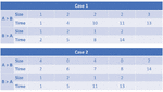
In this work, a traffic analysis system, Packet Momentum, is proposed to identify anonymity networks based on first N-packets. In this section, the features to represent the traffic are introduced based on the first N-packets. To this end, assume that there are two communications taking place as shown on Figure 1 and Figure 2. Case 1 represents communication between user A and user B for application 1. Case 2 represents communication for application 2. In Case 1 user A sent 5 packets to user B which contain 10 bytes in total. User B sent 4 packets to user A with 6 bytes in total. The numbers used in this example are simplified for the purpose of explaining the features. In Case 2 (another application) user A sent 5 packets as well to user B with 10 bytes in total. User B sent back to user A 4 packets with 6 bytes in total. Based on these values, the total number of packets in both directions, the total bytes sent, the average payload size and the average inter arrival time for the two different applications are exactly the same. The average payload size in Case 1 (A) and Case 2 (A) is identical (equal to 2 bytes). The total bytes sent is identical as well (equal to 10).
Figure 1 Example of packet size and inter arrival time features.
Figure 2 Packets exchange in Case 1 and Case 2.
5 Packet Based Identification for Anonymity Networks
The average inter arrival time between the packets in Case 1 (A) is equal to 3. The average inter arrival time between the packets in Case 2 (A) is equal to 3 as well even though the timing in both cases is totally different.
The same applied to B in both cases where both have the same average inter arrival time which is 4. Consequently, in this particular situation, the average payload size, the number of packets, the average inter arrival time and the number of sent bytes are not enough to distinguish between Case 1 and Case 2. It might be hard in real life to have size, inter arrival time and the number of packets to be identical like this but the point is that even using these different important features might not give enough information to have a clear picture about two different applications.
Features generated by any flow exporter tool have different importance based on the types of applications or traffic under analysis. That means if the features are ranked top-down for one set of applications, then this rank is different for another set of applications. For example, the duration, the number of bytes sent and the maximum packet size were the most important features for describing the flow behavior of Tor pluggable transport [21]. The importance of these features is determined based on a features ranking method called “Ranker” in WEKA [10]. This method could use the information gain to decide the importance of the features. In addition, a decision tree could visualize the importance of the features based on the features information gain. When the idea of information gain is applied to the example given here and according to the value shown in Figure 1, then the information gain for the features (Average Inter Arrival Time, Average Payload Size, Total bytes sent and Number of packets) could not provide any difference for Case 1 and Case 2. Consequently, in this situation these features do not provide useful information for classifying the two applications. The features described below are proposed to address this challenging situation.
5.1 Maximum Packet Size
The highest value for the packet size in Case 1 (A) is 3 whereas it is 2 in Case 1 (B). In Case 2 (A) the maximum packet size is 4 whereas it is 2 in Case 2 (B). It can be seen that the maximum packet size will help to show the difference between Case 1 (A) and Case 2 (A) even when both have the same number of packets and the same average packet size. However, the maximum packet size alone is not enough to distinguish between Case 1 (B) and Case 2 (B) where both have exactly the same size of packets.
5.2 Frequency of Maximum Packet Size
The maximum packet size is a useful feature but it can give more information when combined with the measurement of the influence of the maximum packet size. In Case 1 (A) the maximum packet size is 3 bytes but it appears only once in the communication. In Case 2 (A) the maximum packet size is 4 bytes and it appears twice. By adding the frequency of the maximum packet size, it could describe how strong the effect of this maximum packet size is on the communication.
5.3 Second Maximum Packet Size
In Case 1 (A) the highest packet size is 3 bytes and it appears only once, while the 2-byte packet size appears three times. Consequently, including both the highest packet size and the second highest packet size can give more information about the communication.
5.4 Second Maximum Packet Size Frequency
The highest packet size in Case 1 (A) equals 3 bytes and the second maximum packet size equals 2 bytes. However, the maximum packet size appears only once while the second maxim packet size appears three times. Consequently, adding the frequency of the second maximum packet size will show the repetition factor.
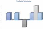
5.5 Packet Sequence
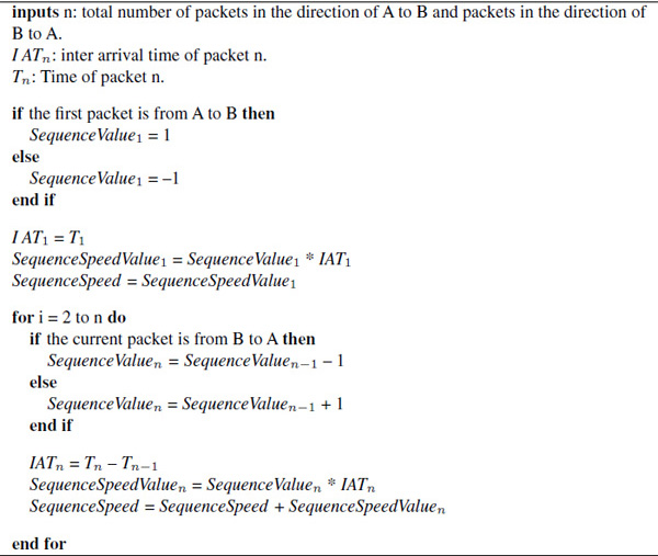
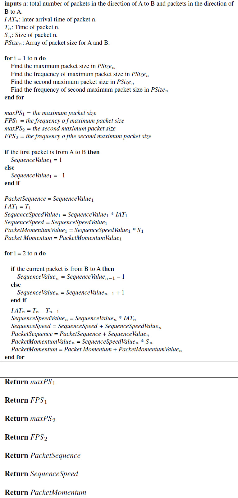
The 4-byte packet in Case 2 (A), which is the maximum packet size, appears twice but not in a sequential order. By contrast, the 2-byte packet, which is the maximum packet size in Case 1 (A), appears three times in a row. The maximum packet size or the second maximum packet size will not show this information. The maximum packet length or the average packet length will not see any difference whether the packets arrive in sequence or not. Consequently, the packet sequence here will describe how the packets arrive in the communication between A and B: it will give more value to the subsequent packets. Figure 3 and Figure 4 show how to present the packet sequence in both cases. The packets will have positive value (1) every time a packet goes from A to B in a cumulative way. If three packets go from A to B in sequence before any packets come from B, then this will add up to (3). Packets from B to A will take the packet sequence down one step, and so on. The packet sequence will be calculated as the summation of all cumulative values. The packet sequence for Case 1 will be 5 and 3 for Case 2. More on calculating the packet sequence can be found in the Appendix section. The Pseudo code for calculating the Packet Sequence is shown in Algorithm 1.
Figure 3 Case 1 packet sequence.
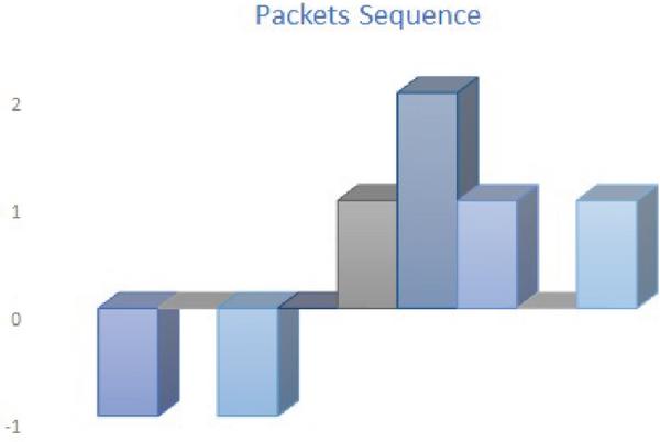
Figure 4 Case 2 packet sequence.
Algorithm 1: Calculation of the Packet Sequence.
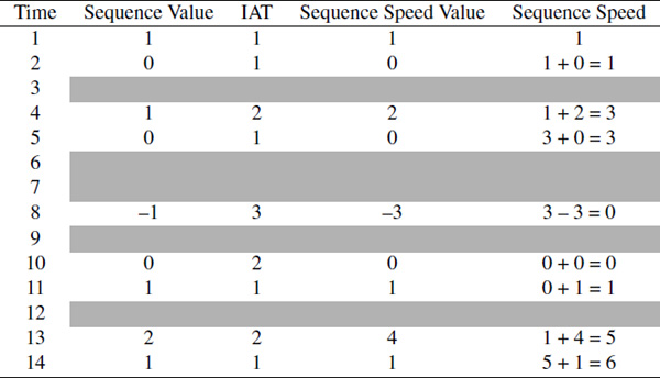
5.6 Sequence Speed
The packet sequence considers the sequence of the packets between A and B, but it does not take into consideration how fast or slow the packets’ flows stay in one direction before the sequence changes. If, for example, three packets arrive in sequence within three minutes, the sequence will have the same value even if these three packets arrive in sequence within 3 seconds. Figure 5 and Figure 6 show how to include the inter arrival time in the calculation to measure the sequence speed. In this way the time needed to change the direction from (A to B) to (B to A) or the opposite will be taken into consideration. The sequence speed reflects the change in direction with respect to the time taken to change the direction and for how long this change stays. The Appendix section shows how to calculate the sequence speed for Case 1. The Pseudo code for calculating the Sequence Speed is shown in Algorithm 2.
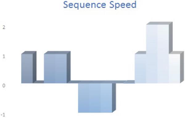
Figure 5 Sequence speed for Case 1.
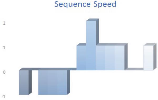
Figure 6 Sequence speed for Case 2.
Algorithm 2: Calculation of the sequence speed.
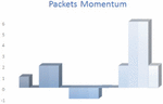
5.7 Packet Momentum
Assume three packets arrive from A to B within 3 seconds with 2-, 3- and 4-byte packets in the first case and another three packets arrive from A to B within 3 seconds (same timing also) 6-, 8- and 9-byte packets in the second case. The sequence speed for both cases will be the same (when the inter arrival time is the same also).
The packet momentum is what takes into consideration the packet size in addition to the sequence and speed. Figure 7 and Figure 8 show the packet momentum for Case 1 and Case 2. The packet momentum distinguishes between packets that have the same inter arrival time and the same sequence.

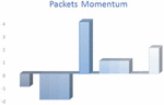
Figure 7 Packet momentum for Case 1.

Figure 8 Packet momentum for Case 2.
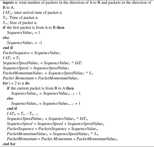
The packet momentum is shown in Algorithm 3. The calculation of the packet momentum for Case 1 is explained in the Appendix section. The pseudo code for all the features of packet momentum is shown in the Appendix section as well.
Algorithm 3: Calculation of the Packet Momentum.
6 Traffic Analysis Using Packet Momentum
The strength of packet momentum analysis relies on two factors: a small number of features and a small number of packets required for the analysis. The number of features has an influence on the calculation cost: the higher the number, the higher the calculation cost. The number of packets needed to analyze the traffic affects the speed of classifying it. For example, the duration of the connection, one of the features employed in the flow analysis for identifying anonymity network traffic [20] and its obfuscated traffic [21], requires that the connection be terminated in order to calculate the duration of the connection. In the Tor pluggable transport analysis, the duration was one of the more important features in the analysis.
The duration of the connection might stay for a brief time or for a very long time. Accordingly, the number of packets in a connection between two parties varies between very low to very large. The packet momentum requires a smaller number of packets for the analysis regardless of the duration of the connection. More details on the number of packets employed in the packet momentum analysis are shown in Section 7. The analysis using packet momentum is described below.
6.1 Anonymity Network Identifications
A binary classification is used here to identify the anonymity network. The first class is the anonymity network which contains anonymity network traffic from Anon17 [3] all combined into one class. This includes the obfuscated traffic of Tor and JonDonym. The second class is non-Anonymity traffic which is the LBNL/ICSI data set [16] where all traffic is labelled as non-anonymity. The LBNL/ICSI contains network traces collected from more than 100 hours of activities for several thousands of hosts. The LBNL/ICSI size is 11 GB distributed over several small PCAP files. In total, 211,370 flows were extracted from approximately 1.5 GB worth of traffic flows. The features employed here are the packet momentum features described previously. The number of packets extracted from each flow and used to calculate the features is 3. In other words, the first 3-packets of each flow is used to perform the classification using the proposed features. By using the C4.5 classifier [18] and 10-fold cross-validation the accuracy was 98.75% as shown in Table 1.
Table 1 Results for binary classification using packet momentum
| TP Rate | FP Rate | TN Rate | FN Rate | |
| Anonymity Traffic | 0.99 | 0.01 | 0.99 | 0.01 |
| Non-Anonymity Traffic | 0.99 | 0.01 | 0.99 | 0.01 |
| Accuracy | 98.75% | |||
Table 2 shows the accuracy of the classifier when using the packet momentum features to classify the anonymity networks (Tor, JonDonym and I2P) in addition to the obfuscated traffic from Tor and JonDonym. In this case, the anonymity networks and the obfuscated traffic are not grouped into one class but labelled separately. The background traffic is the same LBNL/ICSI data set. The accuracy was 98.73%. These results show that the most challenging traffic to classify is Scramblesuit (an obfuscation tool for Tor). However, the proposed approach could still identify the Scramblesuit traffic at 92% detection rate with no false positives.
Table 2 Results of packet momentum for the obfuscated traffic
| TP Rate | FP Rate | TN Rate | FN Rate | |
| Background Traffic | 0.99 | 0.01 | 0.99 | 0.01 |
| I2P | 0.98 | 0 | 1 | 0.02 |
| Tor | 0.94 | 0 | 1 | 0.06 |
| JonDonym | 0.99 | 0 | 1 | 0.01 |
| TCPIPFWD | 0.98 | 0 | 1 | 0.02 |
| SKYPEFWD | 0.99 | 0 | 1 | 0.01 |
| Flashproxy | 0.98 | 0 | 1 | 0.02 |
| FTE | 1 | 0 | 1 | 0 |
| Meek | 1 | 0 | 1 | 0 |
| Obfs3 | 0.97 | 0 | 1 | 0.03 |
| Scramblesuit | 0.92 | 0 | 1 | 0.08 |
| Accuracy | 98.73% | |||
6.2 Identification of Applications and Anonymity Networks
Table 3 shows the performance of the packet momentum when the background traffic is labelled according to the application or the protocol. The anonymity network traffic and the obfuscated traffic also separated in independent classes. Accordingly, there are 22 classes used in this analysis. The result shows a 97.92% accuracy.
Table 3 Results of applications and anonymity networks analysis
| TP Rate | FP Rate | TN Rate | FN Rate | |
| HTTP | 0.97 | 0.01 | 0.99 | 0.03 |
| HTTPS | 0.95 | 0 | 1 | 0.05 |
| IMAPS | 0.81 | 0 | 1 | 0.19 |
| SNMP | 1 | 0 | 1 | 0 |
| NETBIOS-SSN | 0.99 | 0 | 1 | 0.01 |
| DNS | 1 | 0 | 1 | 0 |
| POP3 | 0.80 | 0 | 1 | 0.20 |
| LPD | 0.98 | 0 | 1 | 0.02 |
| EPMAP | 0.99 | 0 | 1 | 0.01 |
| SMTP | 0.99 | 0 | 1 | 0.02 |
| SSH | 0.43 | 0 | 1 | 0.57 |
| OTHER | 0.96 | 0.01 | 0.99 | 0.04 |
| I2P | 0.98 | 0 | 1 | 0.02 |
| Tor | 0.94 | 0 | 1 | 0.06 |
| JonDonym | 0.99 | 0 | 1 | 0.01 |
| TCPIPFWD | 0.99 | 0 | 1 | 0.01 |
| SKYPEFWD | 0.99 | 0 | 1 | 0.01 |
| Flashproxy | 0.98 | 0 | 1 | 0.02 |
| FTE | 1 | 0 | 1 | 0 |
| Meek | 1 | 0 | 1 | 0 |
| Obfs3 | 0.97 | 0 | 1 | 0.03 |
| Scramblesuit | 0.92 | 0 | 1 | 0.08 |
| Accuracy | 97.92% | |||
7 Packet Momentum Validation
One of the factors which influence the time required to build the training and testing models on a classifier is the number of features. In addition, the number of packets employed in the analysis affects the time required for building the models. Also, the number of packets will affect the calculation time for the features. Consequently, the lower the number of features and packets the better the efficiency of the classifier. The following examines these two factors.
7.1 Number of Packets
Table 4 shows the accuracy of the C4.5 10-fold cross-validation for the number of packet changes from 1 to 25 packets. The table includes as well the time needed to build the model, the number of leaves on the decision tree and the tree size. The data employed here is the same data used in Section 6.2 with a total of 22 classes representing the anonymity networks traffic, the obfuscated traffic and the LBNL/ICSI data set as the background traffic labelled as 12 different classes.
Table 4 Influence of number of packets on the packet momentum
| Number of Packets | Accuracy (%) | Time (sec) | Leaves/Tree |
| 1 | 45.8 | 4.4 | 183/365 |
| 2 | 82.5 | 22.53 | 1568/3135 |
| 3 | 97.9 | 15.83 | 1649/3297 |
| 4 | 98.2 | 20.75 | 1497/2993 |
| 5 | 98.3 | 24.01 | 1524/3047 |
| 6 | 98.1 | 25.38 | 1742/3483 |
| 7 | 98 | 27.31 | 1763/3525 |
| 8 | 97.9 | 29.26 | 2109/4217 |
| 9 | 97.9 | 30.69 | 2102/4203 |
| 10 | 97.9 | 28.98 | 1956/3911 |
| 11 | 98 | 28.06 | 1812/3623 |
| 12 | 98 | 29.65 | 1808/3615 |
| 13 | 98 | 31.07 | 1902/3803 |
| 14 | 98 | 31.77 | 1894/3787 |
| 15 | 98 | 31.61 | 1895/3789 |
| 16 | 98 | 28.27 | 1868/3735 |
| 17 | 98 | 28.95 | 1900/3799 |
| 18 | 98 | 28.42 | 1918/3835 |
| 19 | 98 | 28.57 | 1947/3893 |
| 20 | 98 | 27.57 | 1914/3827 |
| 21 | 98 | 29.01 | 1904/3807 |
| 22 | 98 | 28.54 | 1982/3963 |
| 23 | 98 | 31.29 | 2036/4071 |
| 24 | 98 | 31.1 | 2026/4051 |
| 25 | 98 | 29.55 | 1999/3997 |
The results show that packet momentum has the best accuracy with the lowest time to build the model when the number of packets is between 3 and 6. Outside of this range [3–6], the accuracy will drop and the time will increase. When the number of packets was one the accuracy dropped to 45.78%. The reason is that the features of packet momentum will not be utilized. The second maximum packet size will always be zero no matter what application or protocol are analyzed. The frequency of the maximum packet size will always be one for all the classes. When the number of packets is 2, the accuracy improved to 82.53%. Once the number of packets is 3 and above, the accuracy reaches 97%.
7.2 Number of Features
Based on the results of the number of packets in the previous section which shows that a number between 3 and 6 packets gives the better performance for packet momentum, the number of features will be analyzed for the same range of packets (3–6). WEKA’s InfoGianAttributeEval will be used as the method for evaluating the attributes. The search method is the WEKA’s Ranker. Table 5 shows the ranking of the features when the number of packets is between 3 and 6 packets.
Table 5 Features ranking for packets between 3 and 6
| Number of Packets | Features Ranking |
| 3 | 5,1,10,11,8,4,9,6,7,3,2 |
| 4 | 5,1,10,11,4,6,8,2,9,7,3 |
| 5 | 1,5,10,2,6,11,4,8,9,3,7 |
| 6 | 5,1,10,6,2,11,4,8,9,7,3 |
Table 6 shows the accuracy and the time needed to build the model when the number of features is reduced. One feature will be removed at a time based on the ranking in Table 5. Starting from 11 features until only one feature remains, the accuracy and the time needed to build the model will be measured for 3, 4, 5 and 6. Mostly, removing a feature from the features list will reduce the time needed to build the model. At the same time the accuracy decreases for each feature removed from the features list. A high drop in the accuracy happens when the number of features is reduced from 3 to 2. The highest drop in the accuracy appears when reducing the number of features to only one feature.
Table 6 Measurement of packet momentum performance for the number of packets vs the number of features
| 3 Packets | 4 Packets | 5 Packets | 6 Packets | |||||
| Acc | Time | Acc | Time | Acc | Time | Acc | Time | |
| No of Features | (%) | (sec) | (%) | (sec) | (%) | (sec) | (%) | (sec) |
| 11 | 97.9 | 15.83 | (%) | 20.75 | 98.3 | 24.01 | 98.1 | 25.38 |
| 10 | 97.9 | 16.51 | 98 | 16.95 | 98.2 | 21.1 | 98 | 20.07 |
| 9 | 97.9 | 14.44 | 98 | 18.57 | 98.1 | 20.06 | 98 | 21.82 |
| 8 | 97.8 | 15.6 | 98 | 17.43 | 98.1 | 17.92 | 97.9 | 20.11 |
| 7 | 97.8 | 14.92 | 98 | 16.98 | 98 | 16.19 | 98 | 18.32 |
| 6 | 97.8 | 14.17 | 98 | 14.87 | 97.9 | 15.48 | 97.8 | 17.03 |
| 5 | 97.7 | 13.09 | 97.6 | 15.23 | 97.9 | 13.55 | 97.8 | 14.88 |
| 4 | 97.6 | 12.78 | 97.3 | 15.59 | 97.6 | 12.82 | 97.3 | 16.25 |
| 3 | 97.2 | 10.65 | 97.1 | 12.95 | 96.8 | 14.72 | 96.3 | 16.77 |
| 2 | 92.4 | 7.81 | 93.1 | 9.63 | 93 | 11.04 | 92.6 | 11.91 |
| 1 | 84.3 | 4.01 | 85.1 | 4.76 | 83.2 | 5.71 | 83.3 | 5.09 |
8 Performance under Different Classifiers
The C4.5 Decision Tree was the classifier employed in the aforementioned analyses in the previous sections using packet momentum. Table 7 shows the performance of packet momentum when using 10-fold cross-validation for C4.5, Random Forests [5], Naive Bayes [30] and Bayesian Network [8]. The performance was measured for the 22 classes as in Section 6.2.
Table 7 Performance of Packet Momentum under different classifiers
| C4.5 | Random Forest | Naive Bayes | Bayesian Network | |
| Accuracy (%) | 97.92 | 98.25 | 39.2 | 90.58 |
| Time (sec) | 19.02 | 142.6 | 0.56 | 3.9 |
The performance of C4.5 (97.92 %) was increased to 98.25% when using Random Forests, while the time needed to build the model increased from 19.02 seconds to 142.6 seconds. Apparently, the increase in accuracy that Random Forests offers (0.33%) which is less than 1% does not substitute the increased time in building the model. Naive Bayes had the lowest time to build the model (0.56 seconds) but the performance suffered (39.2%). Bayesian Network has a balance performance between the time needed to build the model (3.9 seconds) and the accuracy (90.58%). Compared to Naive Bayes, Bayesian Network has much better performance but still, C4.5 is the best choice based on the trade-off between time and accuracy.
A paired T-test [15] was run on the four classifiers in Table 7 to compare the performance (accuracy) of these classifiers when using the packet momentum for the 22 classes. C4.5 was used as a baseline scheme in a pair-wise comparison of the classifiers. 10-Fold Cross Validation was used for the four classifiers. Then, this procedure was repeated ten times which lead to the generation of 400 results. The test aims to provide evidence to reject the null hypothesis which means the accuracy of a classifier is statistically significantly better or worse than C4.5. As shown in Table 8 the confidence level in the test was 95% (0.05 significance level). The test shows that Random forest with a 98.2% accuracy was statistically significantly better than C4.5 with a 97.9% accuracy. Naive Bayes with a 39.2% accuracy was statistically significantly worse than C4.5. Bayesian Network with a 91% accuracy was statistically significantly worse than C4.5.
Table 8 T-Test result for the accuracy of the C4.5 classifier compared to other classifiers
| T-Test, Significance Level = 0.005, 10-Times 10-Fold Cross Validation | |||
| Classifier | Random Forest | Naive Bayes | Bayesian Network |
| Statistically significant | Better | worst | worst |
| Accuracy | 98.2% | 39.2% | 91% |
9 Conclusion
This research proposes Packet Momentum which employs a machine learning approach using a set of features based on the first 3-packets of a network traffic flow to identify multilayer-encryption anonymity networks. Packet Momentum aims to provide the suitable features that could provide sufficient information to identify multilayer-encryption anonymity networks efficiently. The proposed features in Packet Momentum are Maximum Packet Size, Frequency of Maximum Packet Size, Second Maximum Packet Size, Frequency of Second Maximum Packet Size, Packet Sequence, Sequence Speed and Packet Momentum. The Packet Momentum features were tested on identifying multilayer-encryption anonymity networks and showed high accuracy. Moreover, the results of using Packet Momentum on identifying applications running on the anonymity networks and on identifying obfuscated traffic used on anonymity networks showed that Packet Momentum is efficient for identifying such traffic as well.
Packet Momentum could use as few as three packets to identify multilayer-encryption anonymity networks with a high accuracy. The number of features in the Packet Moment approach is eleven. These features are fewer than the number of features employed previously in experiments on multilayer-encryption anonymity networks. The features have been inspired by the analysis and experiments of this research. For example, the traffic flow analysis of the Tor network highlights the fact that Tor uses fixed-size cells to communicate and carry data. This behaviour has its reflection in the packet sizes that Tor shows in the traffic analysis. Consequently, maximum packet size and its frequency are included in the Packet Momentum features set. Furthermore, the regular approach for the anonymity user to include obfuscated traffic in the connection to the anonymity network starts with the user sending a connection request to the obfuscation server and waiting for a response. By contrast, Flashproxy starts the connections to the user, not the other way around. This example of communication behaviour inspired the use of sequence and sequence speed. Finally, the results show that the features on Packet Momentum demonstrated a high accuracy on different data sets. Future research will continue to analyze the performance of Packet Momentum on a larger scale. The implementation of this approach also will be investigated in a network tool used to identify anonymity networks. The Packet Momentum tool will be studied as well for identifying applications in conjunction with other anonymity networks.
Appendix
Calculation of the Features on Packet Momentum
The following shows the calculation of the features on Packet Momentum.
Calculation of Packet Sequence
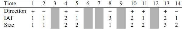
As shown in Section 5.5, the packet sequence feature calculates how strong is the change in the packet direction between two communication parties, A and B. Packet Sequence takes into consideration the number of times the packets keep going in one direction. To explain how to calculate the Packet Sequence for Case 1 in Section 5, the packets can be arranged according to the direction, as shown in Table 9. The time is not taken into consideration when calculating how long the packets stay in one direction. The time is used here only to find the change in the direction of the packets. The (+) sign means that the packet direction is from A to B. The opposite is true for the (–) sign. No packets arrived at 3, 6, 7, 9 or 12 seconds, so the table’s cells are highlighted in gray to show that. Based on the sign which indicates the direction, one is added whenever there is a (+) sign and one is subtracted whenever there is a (–) sign. At the end all the values of the direction change are added together to find the packet sequence. Table 10 shows the value of the direction each time a change in the direction is happening. Instead of using the time from 0 to 14 seconds, which is the time that the packet originally arrived at A or B, the change in direction will be used. At the first packet the sequence value in Table 10 is set according to the direction of the packet (A to B). For the next packets, if the direction does not change, the sequence value is increased by one. When the direction changes (B to A), the sequence value is reduced by one, and so on. The packet sequence is the summation of all the sequence values. In this case, the packet sequence is 5.
Table 9 Direction of packets for Case 1
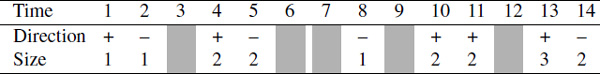
Table 10 Final calculations of packet sequence
| Packet | Sequence Value | Direction | Packet Sequence |
| 1 | 1 | A to B | 1 |
| 2 | 0 | B to A | 1 + 1 = 1 |
| 3 | 1 | A to B | 1 + 1 = 2 |
| 4 | 0 | B to A | 2 + 0 = 2 |
| 5 | –1 | B to A | 2 + (–1) = 1 |
| 6 | 0 | A to B | 1 + 0 = 1 |
| 7 | 1 | A to B | 1 + 1 = 2 |
| 8 | 2 | A to B | 2 + 2 = 4 |
| 9 | 1 | B to A | 4 + 1 = 5 |
Calculation of Sequence Speed
To calculate the Sequence Speed for Case 1, it is necessary to add the inter arrival time from Table 9 as shown in Table 11:
Table 11 Direction and Inter Arrival time for Case 1
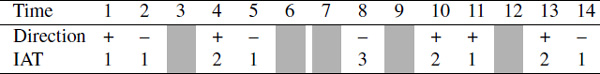
The direction in Table 11 is the same as in Table 9. The inter arrival time is the difference between the time of two consequent packets and it is independent of the direction. In the calculation of the sequence speed the change of direction will be measured with the inter arrival time. Then the summary of all these values will be added to find the sequence speed. Table 12 shows the calculation of the sequence speed for Case 1. The column “Sequence Value” in the table represents the cumulative direction change for each instance of a packet arriving at that time. The column “Sequence Speed Value” is the multiplication of the IAT with the “Sequence Value”. Finally the Sequence Speed is calculated by adding all the results in the “Sequence Speed Value” column. The sequence speed in Case 1 is 6.
Table 12 Calculation of the Sequence Speed for Case 1
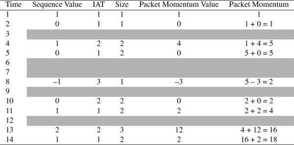
Calculation of Packet Momentum
The packet momentum includes the size of the packets when evaluating the direction and time of the packets. The size is used to scale the amount of change up or down (in the direction of the communication between A and B, in this case). Table 13 shows the size of the packets in Case 1 to be used in the packet momentum calculation. The table includes as well the Inter Arrival time and the direction of the packets taken from Table 11.
Table 13 Size, Time, Direction and Inter Arrival time for Case 1
The calculation of the packet momentum requires knowing the size of the packets, the inter arrival time and the packet sequence. The latter has been calculated earlier and could be used to calculate the packet monument. Table 14 shows how to calculate the packet momentum from the required values. The first two columns in the table are the same from the previous calculation of the sequence speed. The third column is the size of the packets at the time the packets arrive. The packet momentum value is the multiplication of the size, the inter arrival time and the sequence value. Finally, the packet momentum is calculated by the summation of all the column “packet momentum value”.
Table 14 Calculation of Packet Momentum for Case 1
Packet Momentum Pseudo Code
Algorithm 4 shows the Pseudo code of all the features of Packet Momentum.
Algorithm 4: Pseudo Code of all Packet Momentum Features.
Acknowledgment
This research is partially supported by the Natural Science and Engineering Research Council of Canada (NSERC) grant, and is conducted as part of the Dalhousie NIMS Lab at http://projects.cs.dal.ca/projectx/. The first author would like to thank the Ministry of Higher Education in Saudi Arabia for his scholarship.
References
[1] Dhiah el Diehn, A.-T., Pimenidis, L., Schomburg, J., and Westermann, B. (2009). “Usability inspection of anonymity networks,” in Proceedings of the Privacy, Security, Trust and the Management of e-Business, 2009. CONGRESS’09. World Congress on, IEEE, Rome, 100–109.
[2] Hyun-Min, A., Kim, M. S., and Ham, J. H. (2013). “Application traffic classification using statistic signature,” in Proceedings of the Network Operations and Management Symposium (APNOMS), Asia-Pacific, Beijing, 1–6.
[3] Anon17. (2017). Anonymity networks dataset. Available at: https://web.cs.dal.ca/∼shahbar/data.html
[4] Laurent, B., and Teixeira, R. (2007). Early recognition of encrypted applications. Pass. Act. Netw. Meas. 2007, 165–175.
[5] Leo, B. (2001). Random forests. Mach. Learn. 45, 5–32.
[6] David, C. (1981). Untraceable electronic mail, return addresses, and digital pseudonyms. Commun. ACM, 24, 84–90.
[7] Roger D., Mathewson, N., and Syverson, P. (2004). “Tor: The second-generation onion router,” in Proceedings of the 13th Conference on USENIX Security Symposium – SSYM’04, Vol. 13, Berkeley, CA: USENIX Association, 21.
[8] Nir F., Geiger, D., and Goldszmidt, M. (1997). Bayesian network classifiers. Mach. Learn. 29, 131–163.
[9] Rentao G., Wang, H.,and Ji, Y. (2010). “Early traffic identification using Bayesian Networks,” in Proceedings of the Network Infrastructure and Digital Content, 2010 2nd IEEE International Conference on, Berkeley, CA, 564–568.
[10] Mark H., Frank, E., Holmes, G., Pfahringer, B., Reutemann, P., and Witten, I. H. (2009). The WEKA data mining software: An update. SIGKDD Explor. Newsl. 11, 10–18.
[11] Chang, H., Hong, S., and Hong, Z. (2013). “Early recognition of internet service flow,” in Proceedings of the Wireless and Optical Communication Conference (WOCC), Chengdu, 464–468.
[12] I2P. (2017). The Network Database. Available at: https://geti2p.net/en/docs/how/network-database
[13] Zhen, L., Luo, J., Yu, W., and Fu, X. (2011). “Equal-sized cells mean equal-sized packets in Tor?,” in Proceedings of the Communications (ICC), 2011 IEEE International Conference on, IEEE, London, 1–6.
[14] Petar M., and Kademlia, M. D. (2002). “A peer-to-peer information system based on the xor metric,” in Proceedings of the International Workshop on Peer-to-Peer Systems, Berlin: Springer, 53–65.
[15] Claude N., and Bengio, Y. (2001). Inference for the generalization error. Mach. Learn. 2001, 10–15.
[16] Ruoming, P., Allman, M., Paxson, V., and Lee, J. (2006). The devil and packet trace anonymization. ACM SIGCOMM Comput. Commun. Rev. 36, 29–38.
[17] Project: AN.ON âAS anonymity. (2016). Available at: http://anon.inf.tu-dresden.de/index
[18] Quinlan, J. R. (1993). C4.5: Programs for Machine Learning. San Francisco, CA: Morgan Kaufmann Publishers Inc.
[19] Thorsten, R., Panchenko, A., and Engel, T. (2011). “Comparison of low-latency anonymous communication systems: practical usage and performance,” in Proceedings of the Ninth Australasian Information Security Conference. Australian Computer Society, Inc, 77–86.
[20] Khalid, S., and Zincir-Heywood, A. N. (2014). “Benchmarking two techniques for Tor classification: Flow level and circuit level classification,” in Proceedings of the 2014 IEEE Symposium on Computational Intelligence in Cyber Security (CICS), Orlando, FL, 1–8.
[21] Khalid, S., and Zincir-Heywood, A. N. (2015). “Traffic flow analysis of Tor pluggable Transports,” in Proceedings of the 2015 11th International Conference on Network and Service Management (CNSM), Barcelona, 178–181.
[22] Talieh, S. T., Karray, F., and Kamel, M. (2012). “Early internet traffic recognition based on machine learning methods,” in Electrical & Computer Engineering (CCECE), 2012 25th IEEE Canadian Conference on, IEEE, Barcelona, 1–5.
[23] The Invisible Internet Project (I2P). (2016). Available at: https://geti2p.net/en/
[24] Tor Obfs3. (2017). Available at: https://gitweb.torproject.org/pluggable-transports/obfsproxy.git/tree/doc/obfs3/obfs3-protocol-spec.txt
[25] Tunnel implementation. (2017). Available at: https://geti2p.net/en/docs/naming
[26] Unidirectional tunnels. (2016). Available at: https://geti2p.net/en/docs/tunnels/unidirectional
[27] Cynthia, W., Wagener, W., State, R., Dulaunoy, A., and Engel, T. (2012). Breaking Tor anonymity with game theory and data mining. Concurr. Comput. 24, 1052–1065.
[28] Rolf, W., Herrmann, D., and Federrath, H. (2007). Performance comparison of low-latency anonymisation services from a user perspective. In International Workshop on Privacy Enhancing Technologies, Berlin: Springer, 233–253.
[29] Philipp, W., Pulls, T., and Fuss, J. (2013). “ScrambleSuit: A polymorphic network protocol to circumvent censorship,” in Proceedings of the 12th ACM Workshop on Workshop on Privacy in the Electronic Society, New York, NY: ACM, 213–224.
[30] Xindong, W., Kumar, V., Quinlan, J. R., Ghosh, J., Yang, Q., Motoda, H. (2008). Top 10 algorithms in data mining. Knowl. Inf. Syst. 14, 1–37.
Biographies
Khalid Shahbar is a Ph.D. student at Dalhousie University, Halifax, Canada. He received the B.Eng. degree in electrical engineering from King Abdulaziz University, Jeddah, KSA, in 2001, and the M.Sc. degree in computer engineering from King Saud University, Riyadh, KSA, in 2012. His research interests focus on machine learning, network data analysis and network security.

Nur Zincir-Heywood is a Full Professor of Computer Science at Dalhousie University. She is the Director of Dalhousie Network Information Management and Security (NIMS) Lab. Her research interests include data driven techniques for cybersecurity and network management. She is on the editorial board of the IEEE Transactions on Network and Service Management. She has been a co-organizer for the IEEE/IFIP International Workshop on Analytics for Network and Service Management since 2016, and for the ACM Workshop on Genetic and Evolutionary Computation in Defense, Security and Risk Management since 2014. Dr. Zincir-Heywood is a member of the IEEE and the ACM and a recipient of the 2017 Women Leaders in the Digital Economy Award.
Journal of Cyber Security, Vol. 6_1, 27–56.
doi: 10.13052/jcsm2245-1439.612
This is an Open Access publication. © 2017 the Author(s). All rights reserved.