Analytic Study of Features for the Detection of Covert Timing Channels in NetworkTraffic

Félix Iglesias Vázquez, Robert Annessi and Tanja Zseby

CN Group, Institute of Telecommunications, TU Wien, Austria

E-mail: felix.iglesias@nt.tuwien.ac.at; robert.annessi@tuwien.ac.at; tanja.zseby@nt.tuwien.ac.at

Received 30 November 2017; Accepted 3 December 2017;
Publication 18 December 2017

Abstract

Covert timing channels are security threats that have concerned the expert community from the beginnings of secure computer networks. In this paper we explore the nature of covert timing channels by studying the behavior of a selection of features used for their detection. Insights are obtained from experimental studies based on ten covert timing channels techniques published in the literature, which include popular and novel approaches. The study digs into the shapes of flows containing covert timing channels from a statistical perspective as well as using supervised and unsupervised machine learning algorithms. Our experiments reveal which features are recommended for building detection methods and draw meaningful representations to understand the problem space. Covert timing channels show high histogram-distance based outlierness, but insufficient to clearly discriminate them from normal traffic. On the other hand, traffic features do show dependencies that allow separating subspaces and facilitate the identification of covert timing channels. The conducted study shows the detection difficulties due to the high shape variability of normal traffic and suggests the implementation of semi-supervised techniques to develop accurate and reliable detectors.

Keywords

Covert timing channels
Network traffic analysis
Classification
Anomaly detection
Feature selection

1 Introduction

Covert channels are parasitic communication channels, which are exploited to hide the existence of actual communications but for the senders and the receivers of the covert information. They are parasitic because they are built on top of other systems, usually related to technology or information transmission means. In the case of TCP/IP protocols, covert channels use either TCP/IP header fields or time properties of network traffic packets to hide the secret message.

The existence of covert channels is usually—but not necessarily—related to illegal and criminal activities, e.g., data leakage, malware propagation, penetration attacks. One example is the network attacks during December 2015 on Ukraine power companies, whose computers were infected with Gcat. The Gcat malware created covert channels on Gmail applications to conceal C&C (command-and-control) operations and to pass unperceived by security systems [8]. Covert channels are a serious problem related to security and system vulnerabilities; not in vain, they were already identified as a security threat for communication networks almost 40 years ago [25].

This work focuses on covert channels over TCP/IP and, specifically, on covert timing channels, i.e., whenever time properties of TCP/IP transmissions are exploited. We continue the investigations started with [12], where covert channels were classified by studying the implications and challenges faced from the detection side. Additionally, in [12] a general solution for covert channel identification called DAT (from Descriptive Analytics of Traffic) is proposed. The DAT methodology is based on representing traffic flows with a set of statistical measurements and estimations. In [13] and [15] the scope was reduced to timing channels, analyzing and testing the detection with supervised classification in [13] and with unsupervised algorithms in [15]. Even in spite of the fact that covert timing channels are anomalies from a semantic understanding, from the perspective of statistical properties they remain in zones also occupied by normal traffic, yet they can be differentiated by supervised analysis (as shown in [15]). In other words, the separation boundaries between traffic flows with and without covert timing channels are not located in low density areas of the problem space (at least when analyzing the spaces created by the features studied in [15]).

In this paper, we extend the experiments and improve the cited research in [12, 13, 15] as follows:

Study of new features for randomness and predictability

The suitability of five new coefficients related to the estimation of randomness and predictability in time series is studied. The addition of new features to the basic DAT vector format increases computational costs but is expected to enhance detection performance, being therefore justified in environments that demand high security and deal with assumable traffic volumes.
Validation with novel techniques

A validation phase was added to the experiments. In the validation phase, in addition to the eight covert timing techniques used in previous experiments, detectors are evaluated versus two new covert timing channels published in 2017, which are not present during training and testing phases. The robustness of statistical detection frameworks is therefore here tested as well as the hypothesis that suggests that different covert timing techniques are prone to similarly exploit the timing capacities of network traffic (within the scope of the features undertest).

The rest of the paper is organized as follows: Section 2 briefly describes the covert timing channel techniques used in the experiments. Section 3 describes the features under study. Section 4 depicts the experimental design andSection 5 discusses the obtained results. Finally, conclusions are drawn inSection 6.

2 Explored Covert Timing Channel Techniques

For the experiments we have selected ten covert timing channel techniques. Eight of them are popular in the field of covert channel detection, widely described in [13] and in the original papers (we provide the corresponding references). The last two techniques have been published recently in [7]. We use them here for validation and testing detectors against unknown/novel techniques. We abbreviate technique names with three capital letters (or two and one number) that refer to the authors who published them. Techniques are briefly described later in this section, and Table 1 lists the specific parameters used for the generation of covert channels.

For a better understanding of the developed methods, it is important to clarify two different terms related to time properties. The Inter Arrival Time (IAT) refers to the time between packets seen from the perspective of the receiver; on the other side, the Inter Departure Time (IDT) is the time between packets seen from the perspective of the sender. Synthetically expressed: IAT = IDT + tx_delay, where “tx delay” is the transmissiondelay.

2.1 Packet Presence (CAB)

In this technique communication partners are time synchronized and agree on a predefined time interval t_int. The presence or absence of a packet within the predefined time interval stands for the covert symbol 1 or 0 respectively [4].

2.2 Differential/Derivative (ZAN)

This is a technique originally described for the Time-to-Live (TTL) field [33], yet easily applicable to IATs. This technique makes use of two parameters, t_b and t_inc. t_b refers to the base IDT at which packets may be sent and t_inc to the time that may be added or substracted from t_b. If the covert symbol 0 is to be transmitted, the IDT is set to t_b; if the covert symbol 1 is to be transmitted, however, the IDT is set to t_b ± t_inc. Addition and substraction are applied alternately on subsequently occurring 1 symbols.

2.3 Fixed Intervals (BER)

This straightforward technique [1] agrees on two different IDTs to mask binary symbols. For instance, t₀ for 0 and t₁ for 1.

2.4 Jitterbug/Modulus (SHA)

The technique [28] is designed to interfere legitimate communications. It uses a base sample interval ω and adds some delay to IDTs. A covert 1 or a 0 is interpreted depending on if a given IAT is divisible by ω or only by ω/2.

2.5 Huffman Coding (JIN)

By using Huffman coding, every covert symbol is encoded in a set of packets with different IDTs [32]. The proposed codification tries to optimize communication bandwidth based on the frequency of ASCII symbols observed in English texts. The given implementation only covers a set of basic lower case characters and numbers.

2.6 One Threshold (GAS)

This technique [9] uses a time threshold t_h to discriminate 0s and 1s. If a given IAT is above t_h it will mark 1, 0 if below. For the implementation we used additional times to create the covert channel and match the proposed rule (Section 1).

2.7 Packet Bursts (LUO)

In this technique [20] packets are sent in bursts. The number of packets sent per burst marks the intended covert symbol to transmit. Between two subsequent bursts, some time t_w is waited. In principle, this technique is not exploited for binary channels, but manages some symbols (few, about 10 or 16).

2.8 TCP Timestamp Manipulation (GIF)

This technique [10] uses TCP timestamps to convey covert information. Packet IDTs are altered in such a way that the least significant bit (LSB) of the TCP timestamp matches the covert information. TCP timestamps are updated at a specific clock frequency, usually 100, 250, or 1000 Hz. For this reason, this technique establishes a waiting t_b between consecutive packets (authors suggest a minimum of 10 ms). If the LSB is the same as the desired numerical covert symbol, the packet is sent; if not, the sender checks the LSB again after a defined t_w.

2.9 ASCII Binary Encoding (ED1)

This technique [7] encodes the covert symbol 0 with a waiting time t₀ (authors suggest 300 ms), whereas the covert symbol 1 triggers the immediate sending of a packet. Note that t₀ is not defining any IDT; therefore, sending 0s does not imply sending any packet. For example, if ‘A’, which corresponds to the ASCII encoding ‘01000001’, is to be covertly send, the sender will follow this sequence: (1) wait 300 ms, (2) send one packet, (3) wait 1.5 s (300 ms×5),(4) send one packet. Messages are forced to finish transmitting a ‘1’.

2.10 5-Delay Encoding (ED2)

This technique [7] encodes every letter of the English alphabet with a 5-digit numerical code where each digit corresponds to a different IDT. Authors propose a waiting time between covert letters, t_w.

3 Selected Features

As mentioned in Section 1, a recent classification of covert channels is presented in [12]. Moreover, DAT is introduced as a general methodology to identify covert channels in network traffic flows. The DAT approach is fundamentally based on a set of statistical figures and estimations extracted from TCP/IP flow header fields as well as IATs. The specific field understudy—IAT for the case of covert timing channels—is initially tackled from a time series analysis perspective. Further derived studies that focus on covert timing channels are developed in [13] and [15]. Here we explore the features used in these three cited works ([12, 13] and [15]) and add five new features related to regularity and randomness in time and symbol series.

Before depicting features, it is worth remembering that detectors must define two time parameters to enable time series analysis:

Sampling time, which states the desired binning (time resolution, or granularity) for the time series analysis. DAT detectors and the experiments conducted here work with a 1-millisecond sampling time by default.
Observation period, which establishes the maximum time-window for the observation of a given flow. DAT detectors and the experiments conducted here work with a 5-minute observation period by default.

The feature vector extracted from IATs of analyzed flows is:
$flow_vec= {U, S_{k}, μ_{ω S}, S_{s}, p (Mo), ρ_{A}, H_{a}, T_{R}, T_{S}, H_{q}, K, pkts} (1)$
The meaning of each feature is described below.

3.1 Simple Statistical Figures

U— number of unique values. U stores the number of non-repeated IAT values observed in the analyzed flow.
pkts— total number of packets in the flow. pkts is simply a counter that contains the total number of packets observed in the analyzed flow.
p(Mo)— Mode frequency. p(Mo) is a percentage value calculated as the quotient between the number of IAT Mode value repetitions and the total observed IATs in the flow (i.e., pkts – 1).
c — estimation of potential covert byte-equivalent symbol. The calculation of c is based on empirical tables and tries to estimate the number of potential covert bytes sent in a flow [12]. It uses S_k (defined in Section 3.2) to guess the number of different symbols that the covert channel might be applying. For example, if S_k reveals a possible binary channel, c becomes: c = (pkts –1)/7, assuming that 7 IATs values are necessary to transmit a covert byte-equivalent symbol¹.

An example should help to understand the introduced features. For instance, given the following sequence of IATs in a flow i:

{IAT}_{i} = {5, 15, 14, 4, 5, 6, 16, 15, 5, 15, 14, 15, 4, 5} ms (2)

Feature values would be: U = 6, i.e., the cardinality of the unique values set: {4, 5, 6, 14, 15, 16}; p(Mo) = 4/14 = 0.29, given that the Mode (15) occurs 4 times; pkts = 15; and c = 14/7 = 2, since S_k = 2.

3.2 Multimodality Estimation

Multimodality refers to values that either significantly occur more often than others in the series or appear as attractors in the series distribution. Estimating multimodality means providing the number of such attractors. The features related to multimodality are:

S_k— multimodality based on kernel density estimations. S_k is the number of peaks of the curve that approximates the empirical distribution of IATs by using a gaussian kernel. Figure 1 shows two examples with similar estimated curves and both with S_k = 2. Kernel density estimation for assessing multimodality is widely described in [29], and their application for covert channels is discussed in [12].
S_s — multimodality based on pareto analysis. S_s is the number of outstanding values that appear in the IAT histogram. It follows the principles of Pareto analysis [24] and the specific calculation is depicted in [12]. In short, it is the number of values that show a considerable high frequency compared to the rest of the histogram. Figure 1 shows two examples: in the left one S_s = 2, whereas in the right plot S_s = 6.S_s is expected to be irrelevant for the case of IATs as—considering a millisecond resolution—IAT series distributions tend to look like distributions of continuous variables.
μ_ωS — average distribution width. μ_ωS is the mean of the characteristic standard deviations of the gaussians drawn by the kernel density estimations. More intuitively: it captures the average peak width of the mountains that appear in the empirical distribution.

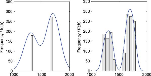
Figure 1 Histograms (bars) and kernel density estimations (curves) of two different numerical series. Left plot: S_k = 2, S_s = 2. Right plot: S_k = 2, S_s = 6. Density magnitudes are omitted as only the number of peaks is relevant for the purpose of the estimation. Figure taken from [12].

3.3 Regularity/predictability Estimators

The coefficients described in this section try to provide an estimation of the randomness, the unpredictability or the regularity of a time series. ρ_A was initially proposed in [12], whereas the other five measurements are added here to test if their inclusion enhances detector performances. In addition to the associated computational costs, the main drawback of all these coefficients is that they require time series be long enough (the minimum threshold is approximately placed between 10 and 100 elements). For short time series, coefficient values are either meaningless or not computable. This fact does not imply a serious problem for covert timing channel detection as, by default, short flows—specially in binary covert channels—cannot contain significant amounts of information and can be directly discarded by the detector. For instance, a binary channel that hides the sentence “hello world!” as 7-bit ASCII characters requires 1 + 12 × 7 = 85 packets (84 IATs).

ρ_A— sum of autocorrelation coefficients. ρ_A is the sum of autocorrelation coefficients, i.e., the IAT time series is paired with delayed versions of itself and correlation coefficients are extracted. Later, such coefficients are summed and a final value is obtained. In short, ρ_A tries to unmask repetition patterns that fit the studied delays. Values close to 1 disclose the existence of patterns and regularity.
T_R — runs test. The runs test [2] checks if it is reasonable to consider that each element in the studied time series is independent and originates from the same distribution. For a non-binary time series A, an intermediate step is required:
$B = A - μ_{A} (3)$
where μ_A is the statistical mean of A. R is the runs of B, i.e., the number of sub-series of negative or positive values within B. Finally,
$Z = \frac{R - E [R]}{S [R]} (4)$
where E[R] is the expected number of runs, and S[R] stands for the expected standard deviation of R. Finally,
$T_{R} = | Z | - Z_{1 - α / 2} (5)$
For time series with more than 20 elements, they are considered non-random if T_R is positive.² This test is widely explained in [2].
T_S — sign test. The sign test [21] is similar to the run test. Given the time series A, instead of counting runs, it takes consecutive pairs of values and constructs a new time series as follows:
$B = A_{2} - A_{1}, A_{3} - A_{2}, \dots, A_{n} - A_{n - 1} (6)$
being n the total number of elements in A. P is the signs of B, i.e., the number of positive elements in B. Therefore,
$Z = \frac{P - E [P]}{S [P]} (7)$
where E[P] is the expected number of signs, and S[R] stands for the expected standard deviation of R. T_S is defined similarly to T_R:
$T_{S} = [Z] - Z_{1 - α / 2} (8)$
where time series with more than 20 elements are considered non-random if T_S is positive.
K — Kolmogorov complexity or compressibility. Given a string, the Kolmogorov complexity is defined as the length of the shortest computer program that generates such string [18]. The calculation of the Kolmogorov complexity, as originally defined, presents problems related to computability. Nevertherless, considering long-enough strings, using lossless compression for approximating Kolmogorov complexity has proven to satisfactorily estimate upper bounds in different domains [19]. In our experiments, we approximate K as:
$K = len (B) / len (A) (9)$
with len(A) being the length of the time series A and len(B) the length of the compressed version of A by zlib³, i.e., B = zlib(A).
H_q — Hurst exponent. The Hurst exponent is strongly linked to the fractal properties of a sequence of values or series, therefore it also provides a measure of autocorrelation and self-similarity. In the case of time series, it gives a quantitative estimation of the trend to regress to the mean value or to be inclined to move in a certain direction [17]. Values between 0.0 < H_q < 0.5 and 0.5 < H_q < 1.0 stand respectively for negative and positive autocorrelations, while H_q = 0.5 corresponds to uncorrelated Brownian processes [6].⁴
H_a — Approximate Entropy. Approximate entropy is a statistical method devised to measure complexity and regularity of a system, which has proven to be suitable for short (but more than 100 data points) and noisy time-series [27].⁵ H_a reflects the existence of patterns in a series that makes future values more predictable. Small H_a values tending to 0 are expected for time series that contain repetitive patterns, whereas high values are expected for chaotic behaviours.

As an example, Figure 2 shows two time series: T1, generated at random, and T2, exhibiting a clear pattern. Regularity/predictability coefficients are shown below the figure.

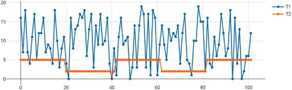
Figure 2 Regularity/predictability coefficients for two example time series.T1: ρ_{A_1.5} = 0.73, T_R = -1.76, T_S = -1.61, K = 1.00, H_q = 0.68, H_a = 2.32.
T2: ρ_{A_1.5} = 0.09, T_R = 7.49, T_S = 14.66, K = 0.31, H_q = 0.71, H_a = 0.08.

4 Design of Experiments

The experiments conducted in this research use real data flows for the traffic free of covert channels (henceforth called overt datasets) and flows with covert channels created by an ad-hoc traffic generation framework (henceforth called overt datasets). We describe them in this section.

As introduced in Section 3, flows are tracked 5 minutes as longest (observation period), and the sampling time for the IAT data is fixed to 1 millisecond. Final preprocessed datasets for experiment replication and further algorithm testing are publicly available to download from ourwebpage in [31].

4.1 Overt Datasets

Real traffic—in principle assumed free of covert channels—has been obtained from the MAWI Working Group Traffic Archive⁶. The MAWI project promotes network traffic research by daily publishing 15 minutes of TCP/IP backbone traces, from 2:00 pm to 2:15 pm GMT. MAWI datasets are anonymized and do not contain payload. We used captures from three days in 2017: a) January 31, b) February 28, and c) March 31, randomly selecting flows to create three overt datasets, namely: nocc_training, nocc_testing and nocc_validation.

Since, for the case of covert timing channels, DAT detectors automatically consider flows with less than 10 packets as overt flows (i.e., they are too short to contain a covert timing channel), all flows with less than 10 packets were removed from the overt dataset. In [13] and [15] flows with less than two packets were removed instead. This difference makes current experiments more demanding and challenging as covert flows are only compared with overt flows that potentially look like covert flows. Performance indices are expected to be worse due to this reason. It is important to remark here that datasets used in the experiments do not try to be representative of real traffic conditions (were the rate of covert channels is absolute negligible), but submit the analysis to problem spaces that are suitable for the knowledge extraction and feature testing.

After preprocessing steps, overt datasets contain 30000 flows in nocc_training, 30000 flows in nocc_testing and 46193 in nocc_validation.

4.2 Covert Datasets

Covert datasets were also generated in three groups, namely:

cc_training (1022 flows), including flows generated by using CAB, BER, SHA, JIN, GAS, LUO, ZAN and GIF techniques.
cc_testing (1036 flows), including flows generated by using CAB, BER, SHA, JIN, GAS, LUO, ZAN and GIF techniques.
cc_validation (1232 flows), including flows generated by using CAB, BER, SHA, JIN, GAS, LUO, ZAN, GIF, ED1 and ED2 techniques.

Each covert dataset was generated with a different set of files to be secretly sent. Each set of files consisted of various types of data, including plain-text (text files, list of passwords, technical reports and programming scripts), images (PNG and JPEG), compressed files (in ZIP and GZ formats), and encrypted files (in 3DES and GnuPG formats). Each singular channel was generated with a different parameterization, random seed and data to be covertly sent. Parameter value ranges were defined according to the original publications (whenever provided); otherwise, they were tuned based on traffic measurement expert knowledge. We also increased some parameter values whenever the source publication did not properly consider transmission delays for large networks. Table 1 shows the value ranges used for the random generation of parameters.

Table 1 Parameters used for the generation of covert channels. Parameters randomly fell within the shown intervals (uniform random distribution)

Technique	Parameters
tx_delay	By default, transmissions delays are modeled with a Lomax (Pareto Type II) distribution with α = 3 ms and λ = 10 ms.
CAB	t_int ∈ [60,140] ms, being t_int the base time window in which the presence or absence of a packet sets the covert symbol.
BER	t₀ ∈ [10, 50] ms, t₁ ∈ [80, 220] ms. t₀ stands for the IDT of covert 0s and t₁ for covert 1s.
SHA	The ground transmission was modeled by using a Gamma distribution with k ∈ [40, 760] ms and ϕ∈ [40, 360] ms. The SHA technique uses ω ∈ [10, 90] ms as sampling interval to manipulate the sending with little delays.
GAS	IDT distribution for 0-packets: t₀ = th - t_sIDT distribution for 1-packets:: t₁ = th - t_s + t_a, th ∈ [100, 300] ms,t_s ∈ [60,140]ms, t_a ∈ [20, 80] ms. th > t_a + t_a
JIN	We used the codification proposed in [32].
LUO	t_w ∈ [50, 250] ms. t_w is the waiting time between bursts. Packets in a burst are sent every ms.
ZAN	t_b ∈ [30, 70] ms, t_inc ∈ [20, 40] ms. t_b is the base IDT between packets. t_inc is added, subtracted or nor applied based on the covert symbol and the previous IDT.
GIF	The minimum time between packets is t_b ∈ [10, 30] ms. The time to recheck TCP timestamps is t_w ∈ [4,12] ms.
ED1	Waiting time for zeros is t₀ ∈ [200, 400] ms.
ED2	Waiting time between covert symbols is t_w ∈ [130,170] ms. The 5-code is built by translating ASCII decimal values into 5-base equivalent numbers. 5-code IDTs: t₀ ∈ [11,19] ms, t₁ = t₀ + t_inc ms, t₂ = t₁ + t_inc ms, t₃ = t₂ + t_inc ms, t₄ = t₃ + t_inc ms, with t_inc ∈ [11,19] ms. The specific numbers have been chosen to deal with path delay variation such that the probability for decoding errors is reduced.

4.3 Analysis Methods

Covert and overt datasets were explored in sequential steps:

Univariate analysis and feature correlation

As a first step, features were studied separately for the cc_training and nocc_training datasets by univariate analysis, aiming to detect noticeable differences in simple statistical figures. Later on, Pearson correlation between features were checked in order to detect distinct feature dependencies in overt and covert traffic.
Feature selection

cc_training and nocc_training were joined in a single training dataset to study feature dependencies with regard to the binary class labels. Features were weighted by feature selection filters and hybrid schemes with different criteria. i.e., decision trees, maximum relevance, information gain, correlation and the gini index—the theoretical background of such indices can be consulted in [26] and [23]. Additionally, feature weighting methods were embedded in a subsampling structure to reinforce result robustness by means of stability selection [22]. Obtained ranks were compared and a final feature set is proposed.
Binary classification and validation

In this phase, training datasets are presented to learners. Obtained models are tested with testing datasets and validated with validation datasets, which explore the effect of including non-trained covert timing channels in the analysis. The training is performed with 10-fold cross-validation, with stratified sampling to keep label proportions in each validation fold. Experiments are repeated with different feature sets to evaluate the results of the feature selection phase. Used learning schemes are: decision trees, random forests, SVMs, neural networks, Bayes-based ensembles and k-Nearest neighbors classifiers.
Unsupervised analysis

Training data is also analyzed by unsupervised outlier detection algorithms in order to see if the new proposed features make covert flows be outliers. Experiments slightly differ from the ones conducted in [15], where overt and covert datasets where presented together to the algorithms. Such experimental scheme might break the normal environment where covert channels appear by overpopulating the space with covert samples (in [15] they consisted on about 5% of the total flows). Covert channels are expected to be much more infrequent among overt data. Therefore, here, outlier detection models are calculated without covert channels, and covert flows are later contrasted with the model and ranked one by one, i.e., every covert flow is isolated and independently compared with the whole overt dataset. Used algorithms are: LOF [3], COF [30], INFLO [16] and HBOS [11]. Used performance indices are: P@n, precision at the top n ranks; Adj.P@n, adjusted P@n; AP, average precision; Adj.AP, adjusted AP; MaxF1, Maximum F1 score; Adj.MaxF1, adjusted MaxF1 score; ROC/AUC, area under the ROC curve. Explanations of such indices can be consulted in [5].

5 Results

The results of the experiments described in Section 4.3 are shown and discussed in this section.

5.1 Univariate Analysis and Feature Correlation

Correlation analysis shows some linear dependencies among the studied features in overt traffic (Figure 3, left plot). Even thought it obviously depends on the features under observation, the characteristics of network traffic make finding high-related features a common situation, as observed in [14]. The positive correlation between the number of U (i.e., unique IATs values) and S_k (i.e., distribution-based multimodes) is not surprising, as well as the correlation between pkts and c, T_R or T_S, which are expected to be higher as the number of packets increase. A special attention deserves indices among the regularity estimators. Entropy measures H_a show inverse correlation with U, which makes sense according to the definition of entropy. The Kolmogorov coefficient K shows inverse correlation with p(Mo) and T_S, which also makes sense because K inversely defines chaos or irregularity if compared to p(Mo) or T_S.

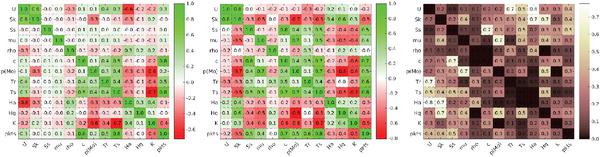
Figure 3 Results of the correlation analysis. Left matrix (A): correlations in the overt dataset. Middle matrix (B): correlations in the covert dataset. Right matrix (C): absolute differences between the correlations in the overt and the covert data set, i.e., c_i,j = |a_i,j - b_i,j|∀i,j being i and j indices for rows and columns, and a_i,j,b_i,j,c_i,j elements of A, B, C respectively.

Table 2 Univariate statistics for overt and covert traffic. Since feature distributions are not Gaussians, we use nonparametric Confidence Intervals (approximately 95%) over the median

	Overt Traffic					Covert Traffic
	mean	stdev	median	CI_low	CI_high	mean	stdev	median	CI_low	CI_high
u	28.75	38.73	15.00	15.00	15.00	196.10	96.17	159.00	155.00	165.00
S_k	18.83	28.88	11.00	11.00	11.00	168.38	114.49	139.00	132.00	146.00
S_s	2.33	6.61	2.00	2.00	2.00	2.62	2.16	2.00	2.00	2.00
μ_ωS	0.01	0.05	0.00	0.00	0.00	0.02	0.04	0.01	0.01	0.01
ρ_A	0.11	0.08	0.10	0.10	0.10	0.04	0.03	0.04	0.03	0.04
c	88.53	1462.21	3.29	3.29	3.29	781.63	2139.75	289.36	246.71	351.00
p(Mo)	0.27	0.22	0.20	0.20	0.20	0.07	0.07	0.05	0.05	0.05
T_R	–0.17	3.57	–1.05	–1.07	–1.02	1.36	4.57	–0.39	–0.50	–0.22
T_S	3.21	18.86	0.00	0.00	0.00	1.87	4.71	0.29	0.10	0.50
H_a	6.95	4.43	10.00	10.00	10.00	0.57	0.06	0.58	0.58	0.58
H_q	129.77	335.41	0.41	0.41	0.41	1.20	0.44	1.29	1.26	1.31
K	0.97	0.12	1.00	1.00	1.00	1.00	0.02	1.00	1.00	1.00
pkts	414.49	4014.59	23.00	22.00	23.00	3647.22	4465.61	1774.00	1615.00	2062.00

The plot in the middle of Figure 3 shows the case of the covert dataset. Covert traffic shows more extreme correlation indices. This fact suggests that covert flows follow more strict and regular structures with respect to the selected features. Another way to look at this picture is acknowledging that overt traffic is richer in shapes and possibilities. Such results foresee a classification scenario where covert flows can be discriminated, but false positives might be also likely. The right plot in Figure 3 shows which features—high values, light backgrounds—might be potentially determinant to establish classification boundaries to separate overt and coverttraffic.

The comparison between univariate analysis of features for overt and covert datasets reveal significant differences in the central tendency measures (Table 2). However, values that significantly differ from overt to covert traffic also show high dynamic ranges (represented by the standard deviation).This fact anticipates overlapping areas in the problem space that can hinder accurate classification.

In short, univariate analysis and correlation tests reveal:

Overt and covert traffic show different central tendencies and feature-correlation profiles. This is an evidence of the existence of patterns that can be learned by classification schemes.
Some feature pairs—specially [U,H_α],[U,T_R],[S_k,H_q],[c,S_s],[p(Mo),μ_ωS]—show opposed correlation relationships when overt and covert traffic are compared. Such pairs might be keys that facilitate the binary classification.
Redundancy is high and common in features, specially for covert traffic. This fact can imply difficulties for selecting the right features and for some classification techniques (e.g., naive Bayes).

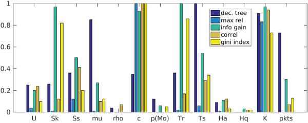
Figure 4 Comparison of feature selection methods.

5.2 Feature Selection

Feature selection experiments expose that features are ranked differently depending on the used feature selection method, as shown in Figure 4. This is not surprising due to the redundancy among features observed during correlation analysis. Nevertheless, all feature selection methods seem to agree in neglecting ρ_A and H_q whereas emphasizing K and c.

The preponderance of K can surprise due to the fact that its correlation relationships among features do not significantly differ when overt and covert traffic are compared each other. In any case, such peculiarity does not imply that K cannot be correlated with the class label. But K is indeed not linearlycorrelated with the class label (ρ = 0.04), and univariate statistics in Table 2 do not show differences between covert and overt traffic for K. Nevertheless, K exhibits a noticeable behaviour change when values are visually compared from an overall perspective (Figure 5).

Summarizing, based on the feature selection analysis we can cluster features in four groups, which remark their importance for distinguishing between covert and overt traffic:

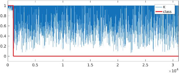
Figure 5 K values throughout covert and overt sample flows.

High relevant: K and c.
Medium relevant: S_k, S_s, T_R, T_S
Low relevant: U, μ_ωS, H_a, p(Mo), pkts.
Negligible: ρ_A and H_q.

As observed in [13], where features are selected by decision trees, c is stated as a decisive feature and ρ_A is neglected. However, with regard to the previous work the importance of other features vary due to the inclusion of the new regularity and randomness features, derived redundancies and the influence of new feature combinations. Also the selection of overt datasets with longer flows, whose characteristics are more similar to covert flows, has an effect on classifiers and feature selection algorithms, which are forced to give solutions with finer granularity.

5.3 Binary Classification and Validation

Based on the feature selection analysis, classification experiments are run to verify the suitability of the selected features. Also, covert channels based on two new techniques are incorporated in a validation step to see if models drawn in training are able to detect novel covert timing techniques, meaning that new covert channels are likely to manipulate traffic capacities in a similar way (from a statistical perspective). Classification is performed with decision tree cores over three different feature sets:

Feature Set A: high, medium, low and negligible features (all).
Feature Set B: high, medium and low relevant features.
Feature Set C: high and medium relevant features.

Table 3 Experiment performance with Feature Set A (all)

	Training		Testing		Validation
	PC	PO	PC	PO	PC	PO
RC	1001 (TP)	21 (FN)	986 (TP)	50 (FN)	1036 (TP)	196 (FN)
RO	40 (FP)	29960 (TN)	41 (FP)	29959 (TN)	96 (FP)	46097 (TN)
Acc.(C):	99.80% ± 0.12%		99.71%		99.38%
Prec.(C):	96.20% ± 2.24%		96.01%		91.52%
Recall(C):	97.95% ± 1.75%		95.17%		84.09%
AUC(C):	0.962 ± 0.099		0.973		0.903

PC: predicted covert, PO: predicted overt, RC: real covert, RO: real overt,
TP: true positive, TN: true negative, FP: false positive, FN: false negative,
(C): covert as positive class, Acc.: accuracy, Prec.: precision, AUC: area under ROC curve.

Table 4 Experiment performance with Feature Set B (excluded negligible)

	Training		Testing		Validation
	PC	PO	PC	PO	PC	PO
RC	997 (TP)	25 (FN)	946 (TP)	74 (FN)	991 (TP)	241 (FN)
RO	37 (FP)	29963 (TN)	96 (FP)	29961 (TN)	81 (FP)	46112 (TN)
Acc.(C):	99.80% ± 0.08%		99.54%		99.32%
Prec.(C):	96.45% ± 1.65%		96.10%		92.44%
Recall(C):	97.56% ± 1.60%		92.86%		80.44%
AUC(C):	0.959 ± 0.100		0.973		0.924

PC: predicted covert, PO: predicted overt, RC: real covert, RO: real overt,
TP: true positive, TN: true negative, FP: false positive, FN: false negative,
(C): covert as positive class, Acc.: accuracy, Prec.: precision, AUC: area under ROC curve.

Table 5 Experiment performance with Feature Set C (excluded negligible and low relevant)

	Training		Testing		Validation
	PC	PO	PC	PO	PC	PO
RC	893 (TP)	129 (FN)	915 (TP)	121 (FN)	980 (TP)	252 (FN)
RO	57 (FP)	29943 (TN)	65 (FP)	29935 (TN)	142 (FP)	46051 (TN)
Acc.(C):	99.40% ± 0.21%		99.17%		99.30%
Prec.(C):	94.23% ± 2.74%		93.37%		87.34%
Recall(C):	87.39% ± 8.07%		88.32%		79.55%
AUC(C):	0.931 ± 0.043		0.920		0.824

PC: predicted covert, PO: predicted overt, RC: real covert, RO: real overt,
TP: true positive, TN: true negative, FP: false positive, FN: false negative,
(C): covert as positive class, Acc.: accuracy, Prec.: precision, AUC: area under ROC curve.

Tables 3, 4 and 5 show performances for every feature set when decision trees are used to create classification models. The revision of such tables disclose some findings:

Table 7 Identification of FN and FP in the validation phase for the relevant feature set

Technique	Wrong	μ_conf(0)	μ_conf(1)
CAB (FN)	8	1.00±0.00	0.00±0.00
BER (FN)	18	1.00±0.00	0.00±0.00
SHA (FN)	2	0.75±0.35	0.25±0.35
GAS (FN)	24	1.00±0.00	0.00±0.00
JIN (FN)	12	1.00±0.00	0.00±0.00
LUO (FN)	8	1.00±0.00	0.00±0.00
ZAN (FN)	11	1.00±0.00	0.00±0.00
GIF (FN)	3	0.78±0.19	0.22±0.19
ED1 (FN)	99	1.00±0.00	0.00±0.00
ED2 (FN)	55	0.70±0.10	0.30±0.10
Overt (FP)	81	0.05±0.09	0.05±0.09
FP: false positive, FN: false negative, wrong: total number of wrong classified flows μ_conf(0) and μ_conf(1) stand respectively for the average decision tree confidence to establish the 0 (overt) or a 1 (covert) label to the misclassified samples.

The performance downgrade when using feature set B (high, medium and low relevant) if compared with the feature set A (all) is minor, likely related to specific non-generalizable cases. From a general perspective H_q and ρ_A can be considered inefficient for detecting covert timing channels and, therefore, removed.
The performance downgrade when using feature set C (high and medium relevant) if compared with the feature set A or B is considerable. Therefore, low relevant features—μ_ωS, H_a, p(Mo), pkts—are still determinant for the classification and should be included regardless of possible redundancies.
The downgrade in the validation phase is obvious in spite of the used feature set. False negatives mainly belong to the novel not-trained techniques ED1 and ED2 (Table 6), meaning that new techniques have room to exploit channel capacities in ways that can bypass classifiers trained with known, old techniques.

Similar test have been carried out with other classifiers, specifically: random forests, SVM, neural networks, Bayes-based ensemble and k-Nearestneighbors learners. A plain decision tree obtained the best performances⁸, yet the previous discussed aspects are common in all tested learning schemes.

5.4 Unsupervised Analysis

Finally, tests by outlier ranking algorithms tried to elucidate if the new considered features could provide extra information to face the detection of covert timing channels from an unsupervised manner. Experiments in [15] revealed that covert timing channels can hardly be seen as outliers. Here, outlier analysis are performed by considering two different feature sets:

Feature Set B: high, medium and low relevant features.
Feature Set D: new high, medium and low relevant features not used in [15], i.e., T_R, T_S, H_a and K.

Results are shown in Table 7 and Figure 6. Results confirm that density-based outlier detection is completely useless for detecting covert timing channels. Only the HBOS algorithm (histogram-based method) can face the task to differentiate between overt and covert flows. However, the probabilities to suspect that a legitimate flow is a covert flow are still too high. For example, the P@n index gives the proportion of correct results in the top n ranks.

Table 7 Outlier detection performance indices for feature set B and D

Feature set B
	P@n	Adj. P@n	AP	Adj. AP	MaxF1	Adj.MaxF1	ROC/AUC
LOF	0.02	–0.01	0.01	–0.03	0.08	0.05	0.55
COF	0.01	–0.02	0.00	–0.03	0.07	0.04	0.53
INFLO	0.02	–0.01	0.01	–0.03	0.08	0.05	0.51
HBOS	0.28	0.26	0.27	0.25	0.49	0.47	0.96
Feature set D
	P@n	Adj. P@n	AP	Adj. AP	MaxF1	Adj.MaxF1	ROC/AUC
LOF	0.04	0.01	0.02	–0.01	0.08	0.05	0.57
COF	0.00	–0.03	0.00	–0.03	0.09	0.06	0.62
INFLO	0.03	0.00	0.02	–0.01	0.07	0.04	0.52
HBOS	0.09	0.06	0.12	0.10	0.36	0.34	0.92

P@n = 0.28 in Table 7 is the best result for the HBOS case, but still too low to build a practical detector. AUC rates are nevertheless significantly high for HBOS. The AUC index can be understood as the probability that the algorithm ranks a randomly chosen positive example higher than a randomly chosen negative example. Summarizing, results show that practically all flows with covert channels obtain high HBOS ranks; overt flows are low-ranked instead, but still some overt flows—a meaningless proportion but still many when compared with covert flows rates—score high and even higher thancovert cases.

Already in [15] HBOS was the only method to find a significant difference between overt and covert flows. The inclusion of the new features (T_R, T_S, H_a and K) reinforces the outlier nature of flows with covert channels, as shown in Figure 6, but is still far from being discriminant.

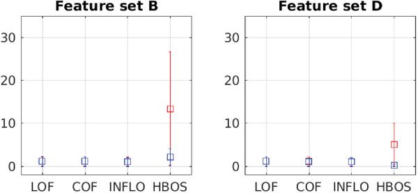
Figure 6 Outlier ranking results. Again, distributions are not normal but strongly skewed. Plots show medians and Confidence Intervals over the median (approximately 95%). Red markers correspond to covert datasets, blue for overt datasets. Red lines are indistinguishable (or almost) in LOF, COF and INFLO due to value overlap.

Therefore, the main findings of the unsupervised experiments are:

As a general trend, covert channel flows obtain higher outlierness ranks when analyzed by the HBOS algorithm (histogram, distance-based), but still a significant proportion of overt flows scores equally high or even higher.
The new features T_R, T_S, H_a and K endorse the outlier nature of covert channels, but the most revealing outlierness ranks are obtained when they are combined and used together with S_k, S_s, c, U, μ_ωS, p(Mo) and pkts.

6 Conclusions

In this work we have deeply analyzed the capacity of some network traffic features to disclose covert timing channels. All analyzed features are measured or calculated from network traffic flows IATs (Inter Arrival Times).

From the analyzed features, the most relevant ones for the detection of covert channels are: c, S_k, pkts and K. c is the estimation of potential covert byte-equivalent symbols, which depends on the number of packets in the flow (pkts) and the number of multimodes that appear in the probability density estimation when using gaussians as kernels (S_k). K is the Kolmogorov complexity estimation approximated by using zlib compression. On the other hand, the hurst coefficient (H_q) and autocorrelation-based coeffcients (ρ_A) are found inefficient and can be discarded.

Conducted experiments show that the detection of covert timing channels is a demanding challenge and new covert techniques can easily bypass trained detection schemes. The high variety of forms that network traffic can take and the extremely low expected rate of covert channels in real traffic are the main reasons that make the accurate detection so difficult. Combination of supervised and unsupervised techniques (i.e., semi-supervise methods) appears as the right direction to follow in order to develop satisfactory detectors. However, a considerable rate of false positives is almost unavoidable unless more complex methods are developed and implemented.

Acknowledgment

The research leading to these results has been partially funded by the Vienna Science and Technology Fund (WWTF) through project ICT15-129, BigDAMA.

References

[1] V. Berk, A. Giani, G. Cybenko, and N. Hanover (2005). Detection of covert channel encoding in network packet delays. Rapport technique TR536, de lUniversité de Dartmouth, 19.

[2] James V. Bradley (1968). Distribution-Free Statistical Tests, 1st Edition. Prentice-Hall.

[3] M. Breunig, H.-P. Kriegel, R. T. Ng, and J. Sander (2000). Lof: Identifying density-based local outliers. SIGMOD Rec. 29, 93–104.

[4] S. Cabuk, C. E. Brodley, and C. Shields (2004). IP covert timing channels: Design and detection. In Proceedings of the 11th ACM Conference on Computer and Communications Security, CCS’04, (ACM: New York, NY, USA), 178–187.

[5] G. O. Campos, A. Zimek, J. Sander, R. J. G. B. Campello, B. Micenkov, E. Schubert, I. Assent, and M. E. Houle (2016). On the evaluation ofunsupervised outlier detection: Measures, datasets, and an empirical study. Data Mining and Knowledge Discovery, 30, 891–927.

[6] A. Carbone, G. Castelli, and H. E. Stanley (2004). Time-dependent hurst exponent in financial time series. Applications of Physics in Financial Analysis 4 (APFA4). Physica A: Statistical Mechanics and Its Applications, 344, 267–271.

[7] E. J. Castillo, X. Mountrouidou, and X. Li (2017). “Time Lord: Covert Timing Channel Implementation and Realistic Experimentation,” inProceedings of the 2017 ACM SIGCSE Technical Symposium on Computer Science Education, SIGCSE’17, (ACM: New York, NY, USA), 755–756.

[8] ElevenPaths. Low cost malware that uses gmail as a covert channel. Telefónica Digital España, Technical report, May 2016.

[9] W. Gasior and L. Yang (2011). “Network covert channels on the android platform,” in Proceedings of the Seventh Annual Workshop on Cyber Security and Information Intelligence Research, CSIIRW’11, (ACM: New York, NY, USA), p. 61:1.

[10] J. Giffin, R. Greenstadt, P. Litwack, and R. Tibbetts (2003). Covert Messaging through TCP Timestamps. Springer: Berlin, Heidelberg, 194–208.

[11] M. Goldstein and A. Dengel (2012). “Histogram-based Outlier Score (HBOS): A Fast Unsupervised Anomaly Detection Algorithm,” in Advances in Artificial Intelligence, (KI-2012), ed. S. Wölfl, pp. 59–63. [Online, 9, 2012].

[12] F. Iglesias, R. Annessi, and T. Zseby (2016). DAT detectors: uncovering TCP/IP covert channels by descriptive analytics. Security and Communication Networks, 9, 3011–3029.

[13] F. Iglesias, V. Bernhardt, R. Annessi, and T. Zseby (2017). “Decision tree rule induction for detecting covert timing channels in TCP/IP traffic,” in First IFIP TC 5, WG 8.4, 8.9, 12.9 International Cross-Domain Conference, CD-MAKE 2017, in (eds) Holzinger A., Kieseberg P., Tjoa A., Weippl E., Lecture Notes in Computer Science, Vol. 10410, ( Springer: Cham), 105–122.

[14] F. Iglesias and T. Zseby (2015). Analysis of network traffic features for anomaly detection. Machine Learning, 101, 59–84.

[15] F. Iglesias and T. Zseby (2017). “Are network covert timing channels statistical anomalies?” in Proceedings of the 12th International Conference on Availability, Reliability and Security, ARES’17, (ACM: New York, NY, USA), 81:1–81:9.

[16] W. Jin, A. K. H. Tung, J. Han, and W. Wang (2006). Ranking Outliers Using Symmetric Neighborhood Relationship. Springer: Berlin Heidelberg, 577–593.

[17] T. Kleinow (2002). Testing continuous time models in financial markets.PhD thesis, Humboldt-Universitát zu Berlin, Wirtschaftswissenschaftliche Fakultt, 2002.

[18] A. N. Kolmogorov (1968). Three approaches to the quantitative definition of information. International Journal of Computer Mathematics, 2, 157–168.

[19] M. Li and P. Vitanyi (1997). An Introduction to Kolmogorov Complexity and Its Applications (Texts in Computer Science). Springer.

[20] X. Luo, E. W. W. Chan, and R. K. C. Chang (2008). “TCP covert timing channels: Design and detection,” in IEEE International Conference on Dependable Systems and Networks with FTCS and DCC (DSN), 420–429.

[21] Henry B. Mann (1945). On a test for randomness based on signs of differences. Ann. Math. Statist. 16, 193–199.

[22] N. Meinshausen and P. Bhlmann (2010). Stability selection. Journal of the Royal Statistical Society: Series B (Statistical Methodology), 72, 417–473.

[23] B. H. Menze, B. M. Kelm, R. Masuch, U. Himmelreich, P. Bachert, W. Petrich, and and F. A. Hamprecht (2009). A comparison of random forest and its Gini importance with standard chemometric methods for the feature selection and classification of spectral data. BMC Bioinformatics, 10, 213.

[24] MEJ Newman (2005). Power laws, Pareto distributions and Zipf’s law. Contemporary Physics, 46, 323–351.

[25] M. A. Padlipsky, D. W. Snow, and P. A. Karger (1978). Limitations of end-to-end encryption in secure computer networks, 1978. ESD-TR-78-158.

[26] H. Peng, F. Long, and C. Ding (2005). Feature selection based on mutual in- formation criteria of max-dependency, max-relevance, and min-redundancy. IEEE Transactions on Pattern Analysis and Machine Intelligence, 27, 1226–1238.

[27] S. M. Pincus (1991). Approximate entropy as a measure of system complexity. Proceedings of the National Academy of Sciences, 88, 2297–2301.

[28] G. Shah, A. Molina, and M. Blaze (2006). “Keyboards and covert channels,” in Proceedings of the 15th Conference on USENIX Security Symposium, USENIX-SS’06, USENIX Association: Berkeley, CA, USA.

[29] B. W. Silverman. Using kernel density estimates to investigate multimodality. Journal of the Royal Statistical Society: Series B, 43, 97–99.

[30] J. Tang, Z. Chen, A. W. Fu, and D. W.-L. Cheung (2002). “Enhancing effectiveness of outlier detections for low density patterns,” in Proceedings of the 6th Pacific-Asia Conference on Advances in Knowledge Discovery and Data Mining, PAKDD’02, (Springer-Verlag: London, UK), 535–548.

[31] TU Wien CN Group. Data Analysis and Algorithms, 2017.

[32] J. Wu, Y. Wang, L. Ding, and X. Liao (2012). Improving performance of network covert timing channel through Huffman coding. Mathematical and Computer Modelling, 55, 69–79, 2012.

[33] S. Zander, G. Armitage, and P. Branch (2007). “An empirical evaluation of ip time to live covert channels,” in 2007 15th IEEE International Conference on Networks, ICON 2007, (IEEE), 42–47.

Biographies

images

Félix Iglesias Vázquez was born in Madrid, Spain, in 1980. He obtained the Dipl.-Ing. in electrical engineering and MAS in IT from the Ramon Llull University, Barcelona, Spain. In 2012 he received the Ph.D. degree in technical sciences from TU Wien, Austria, where he currently holds a University Assistant position doing fundamental research in data analysis and network security. He has worked on R&D for diverse Spanish and Austrian firms, and lectured in the fields of electronics, physics, automation, machine learning and data analysis.

images

Robert Annessi received his B.Sc. and his M.Sc. degrees in computer engineering from TU Wien in 2011 and 2014 respectively. He is genuinely interested in communication networks, network security, and privacy, and is currently pursuing his Ph.D in the area of secure group communication for critical infrastructures. His further research interests are anonymous communication, covert communication, and subliminal communication.

images

Tanja Zseby is a professor of communication networks in the Faculty of Electrical Engineering and Information Technology at TU Wien. She received her Dipl.-Ing. degree in electrical engineering and her Ph.D. (Dr.-Ing.) from Technical University Berlin, Germany. Before joining TU Wien she led the Competence Center for Network Research at the Fraunhofer Institute for Open Communication Systems (FOKUS) in Berlin and worked as visiting scientist at the University of California, San Diego.

¹ It might be surprising the use of “7” instead of “8” in the quotient for estimating byte-equivalent symbols. The c index is an inflated estimation of the transmitted covert information and assumes that it consists of text. In this respect, note that ASCII most relevant/used symbols are less than 2⁷ = 128.

² For a 5% significance level, Z_1-α/2 = 1.96.

³ https://zlib.net/

⁴ For the experiments we have used the hurst implementation from Python library nolds 0.3.4: https://pypi.python.org/pypi/nolds

⁵ For the experiments we have used the approximate entropy implementation from Python library nolds 0.3.4: https://pypi.python.org/pypi/nolds

⁶ http://mawi.wide.ad.jp/mawi/

⁷ It’s worth remembering that c is a function of S_k and pkts.

⁸ The decision tree configuration included pre- and postpruning to avoid overfitting and favor generalization. It used Information Gain (i.e., entropy-based) as splitting criterion; the minimal size for splitting was four samples; the minimal leaf size was two samples, allowing a maximal tree depth of 20 levels; the minimal gain for splitting a node was 0.1; the confidence level used for the pessimistic error calculation of pruning was 0.25, whereas the number of prepruning alternatives was three. In addition, a 10-fold cross-validation process was performed to reinforce disclosed models.