Feature Extraction and Classification Using Deep Convolutional Neural Networks

Jyostna Devi Bodapati¹ and N. Veeranjaneyulu^2,*

¹Assistant Professor, Department of CSE, Vignan’s Foundation for Science, Technology and Research, Vadlamudi, Andhra Pradesh, India

²Professor, Department of IT, Vignan’s Foundation for Science, Technology and Research, Vadlamudi, Andhra Pradesh, India

E-mail: veeru2006n@gmail.com

*Corresponding Author

Received 17 January 2018; Accepted 21 May 2018;
Publication 25 January 2019

Abstract

The impressive gain in performance obtained using deep neural networks (DNN) for various tasks encouraged us to apply DNN for image classification task. We have used a variant of DNN called Deep convolutional Neural Networks (DCNN) for feature extraction and image classification. Neural networks can be used for classification as well as for feature extraction. Our whole work can be better seen as two different tasks. In the first task, DCNN is used for feature extraction and classification task. In the second task, features are extracted using DCNN and then SVM, a shallow classifier, is used to classify the extracted features. Performance of these tasks is compared. Various configurations of DCNN are used for our experimental studies. Among different architectures that we have considered, the architecture with 3 levels of convolutional and pooling layers, followed by a fully connected output layer is used for feature extraction. In task 1 DCNN extracted features are fed to a 2 hidden layer neural network for classification. In task 2 SVM is used to classify the features extracted by DCNN. Experimental studies show that the performance of ν-SVM classification on DCNN features is slightly better than the results of neural network classification on DCNN extracted features.

Keywords

Convolutional neural network
Max pooling
Average pooling
Subsampling
parameter sharing
local connectivity

1 Introduction

All Pattern recognition is the process of identifying patterns in the given data and received increased focus from researcher of this field. In the area of pattern recognition there are many subfields like: Classification, Clustering, regression and dimensionality reduction. These are all highlydemanding tasks in multiple real-time applications [1]. These tasks can be classified as either supervised or unsupervised depending on whether any supervised information is provided while training or not. As supervised information is being used while training, classification and regression tasks fall under the category of supervised learning. In clustering and dimensionality reduction tasks supervised information is not available during training and fall in the category of unsupervised learning.

Regression is a function approximation task in which a continuous value is to be assigned to a given data point. Classification is a type of regression, where the output of the test data is discrete. For classification models like simple K-nearest neighbourhood (KNN), Gaussian mixture models (GMM)-based Baye’s classification [7], artificial neural networks (ANN)-based Multilayer feedforward neural networks (MLFFNN) [10], support vector machine (SVM)-based classification can be used.

Dimensionality reduction is the process of representing high dimensional data in a lower dimensional space. This process can be viewed as projection of data from higher dimensional space to a lower dimensional space. These dimensionality reduction techniques are basically categorized into linear and non-linear methods depending on the way data is projected. Principal component analysis (PCA), Linear discriminant analysis (LDA), ICA, CCA, NMF come under linear dimensionality reduction techniques as the projected data is linearly related to the data in the input space. KPCA [13], KLDA, auto encoders come under non-linear dimensionality reduction techniques, as the projected data is non-linearly related to the data in the input space [3].

Auto associative Neural networks (AANN) are basically feed forward neural networks (FFNN) with structures satisfying the requirements for performing auto-association. Mapping in an AANN [12] is achieved by using a dimension reduction followed by a dimension expansion. Dimension reduction part of the network is called encoder while the dimension expansion part of the network is known as decoder. After training auto-associative neural network, decoder part is removed and encoder part is used for non-linear dimension reduction if the activation function of the hidden layer is non-linear [2].

A convolutional neural network (CNN) is a type of artificial neural network usually designed to extract features from data and to classify given high dimensional data. CNN is designed specifically to reorganize two dimensional shapes with a high degree of invariance to translation, scaling, skewing and other forms of distortion. The structure includes feature extraction, feature mapping and subsampling layers. A CNN consists of a number of convolutional and subsampling layers optionally followed by fully connected output layers. Back propagation algorithm is used to train the model.

Convolution Neural Networks are biologically inspired variants of Multilayer Neural Network [6]. From experiments mentioned in [3] it is known that the visual cortex of animals is a complex network of cells. Each cell is sensitive to small sub-region of the visual fields, known as the receptive field. According to [4], there are two kinds of cells: Simple cells and Complex cells, where simple cells extract features and complex cells combine several such local features from a spatial neighbour-hood. CNN tries to imitate this structure, by extracting the features in a similar way from the input space and then performing the classification, unlike the standard techniques where features are extracted manually and provided to the model forclassification [3].

A 32 × 32 color image can be represented as a 1024 dimensional vector. Considering different values of color (R, G and B), the image can be better represented as a vector of size 4096 (dimensions). To model such high dimensional data using shallow networks involves estimation of large number of parameters. Unless training data is large such models lead to overfitthe data.

Convolutional Neural Network can handle such problems by leveraging the ideas of local connectivity, parameter Sharing and Pooling/Subsampling.

Local Connectivity:

Each image is divided into equal sized units called as blocks or patches. These blocks of the image are also known as receptive fields. These blocks can be overlapping or non-overlapping in nature. Overlapping blocks share some common part of image while non-overlapping blocks do not share. In order to extract smooth features, overlapping blocks are considered. In an image of size 32 × 32 with a block size of 4 × 4 gives a total of 64 blocks.

Each hidden unit is associated with one block of the input image and extracts features from that block of the image. In this way local features are extracted and the exact location of the features become less important. This is beneficial until the relative location with respect to other features is preserved [14]. Figure 1 illustrates an example of local connectivity where each hidden unit is connected to a block or patch of the image.

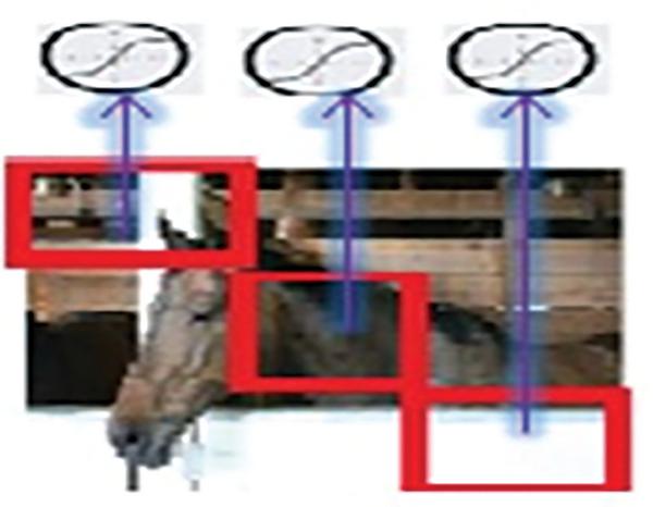
Figure 1 Local connectivity.

Parameter Sharing:

Each computational layer, also known as convolutional layer in the network comprises of a number of feature maps. The neurons in one feature map are constrained to share the same weights. This constraint guarantees: reduction in parameters and shift invariance [15].

This idea of parameter sharing allows different neurons to share the same parameters [16]. To accomplish this task hidden neurons are organized into feature maps that share parameters. Hidden units within a feature map cover different blocks of an image share same parameters and extracts same type of features from different blocks. Each block of an image is associated with multiple feature maps and neurons in different feature maps extract different features from the same block [17].

Figure 2 helps us to clearly understand the process of parameter sharing: Each hidden unit in a feature map is connected to different blocks of an image and extracts same type of features [18]. Hidden units in different feature maps extract different features from the same block [19].

Figure 2 Parameter sharing.

In an image, blocks can be overlapping. To obtain activation values for each hidden unit, weights connecting the input channel to feature map is to be multiplied with input vector. This operation is known as Convolution and basically we are concerned with discrete convolutions.

Discrete Convolution:

Discrete Convolution Operation can be defined as:

h [n] = f (n) * g (n) = \sum_{k = - α}^{α} f [k] g [n - k],

f and g are two functions.

Discrete Convolution is a combination of shift, multiply and addition operations [9]. Here convolution operation is performed by summing up multiplication of the weight matrix with someblock of image and then shifting weight matrix to other overlapping block [20].

Pooling and subsampling:

Pooling works basically in two ways namely max pooling and average pooling. A window of some predefined size is selected in both the methods. In Max pooling, maximum activation value among the values in a window is considered. In Average pooling average of the activation values in a window is considered.

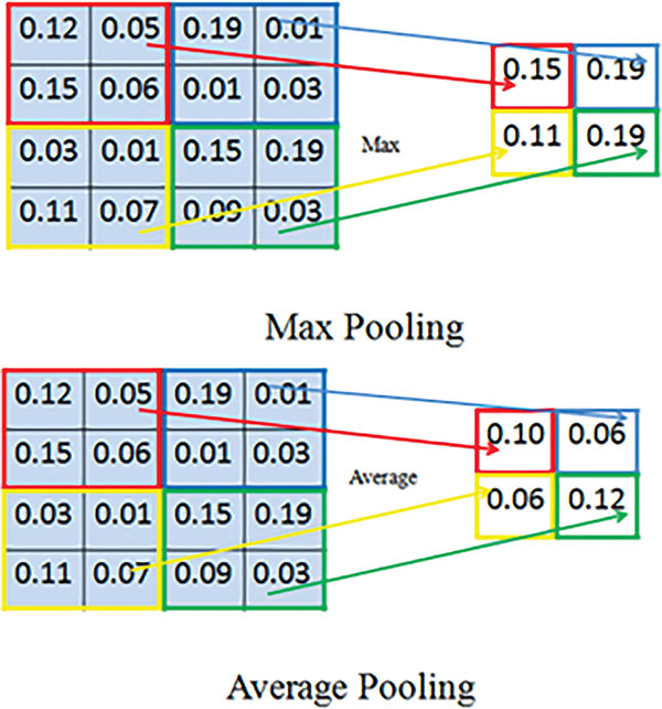
Figure 3 Max and Average pooling.

Max pooling is preferred to average pooling as Max pooling sometimes causes loss of information because it takes maximum value in a local region and maynot be able to give whole information about thatregion [11].

Advantages of introducing pooling layer are: It introduces invariance to local transitions because pooled value remains same in that local neighbourhood. It reduces the number of hidden units in hidden layer as the size of feature maps for the subsequent layers would be smaller. Due to this reduction technique, pooling layer is also called as subsampling layer. Figure 3 illustrates max and average pooling techniques. Consider the input is an 8 × 8 block of activation values and the window is of size 2 × 2. In max pooling, the maximum value from each window is taken and in average pooling average of the activation values in a window is taken. As a result of subsampling 8 × 8 blocks are reduced to a size of 2 × 2 as there are 4 windows and each window results in a single value. This makes the structure invariant to spatialdistortion.

The pooling operation is translation invariant [8], if the regions pooled are from contiguous areas and the regions which are output of the same replicated hidden nodes are chosen. Translation invariance means that the same pooled features will be returned even for small translations in theimages [5].

Figure 4 illustrates the detailed architecture of CNN for classification of 32 × 32 images. This architecture comprises of 3 convolutional and pooling layers followed by a fully connected output layer. In the first convolutional layer receptive field is a 5 × 5 block, and each image is composed of such multiple blocks in an overlapping fashion. Thus each image is described in terms of 28 × 28 overlapping receptive fields. A convolution layer consists of several feature maps, here the first convolution layer consists of 6 feature maps. The neurons in one feature map are constrained to have the same weights to reduce the number of parameters to be estimated. Each neuron thus receives a 5 × 5 input, thus there are 26 features (25 weight parameters and one bias) to be estimated for each feature map.

Figure 4 Sample CNN architecture model.

The next layer is the subsampling layer with a window of size 2 × 2. Input to this layer is a 6 × 28 × 28 matrix and it is reduced to 6 × 14 × 14. Blocks at this stage are non-overlapping. The reduction in the size of the matrix can be performed either by subsampling or by max pooling [3, 4]. Empirical results show that max pooling gives better performance compared to subsampling. The output of the first sampling layer is a 6 × 14 × 14 matrix.

The subsequent layers are two convolutional and subsampling layers with an increase in the number of feature maps and decrease in the spatial resolution. The output layer is a fully connected layer. Output of this layer gives features of the input image. Further classification of these features into classes can be done using any neural network [21].

Dataset used for image classification task:

The task is to classify colored images of dimensions 200 × 200 into 5 classes namely Sheep, Car, Bus, Horse and Boat where each image is of size 3 × 200 × 200. Total number of images in the dataset are 4548.

Table 1 Data set after sampling

Class	Label	Number of Images
1	Sheep	758
2	Car	1042
3	Bus	974
4	Horse	750
5	Boat	1027

The dataset is highly imbalanced, with class 2 and class 5 are having more data points compared to the other classes. So directly applying classification on original data may lead to poor F-score measure as a lot of test cases from the other classes would be classified as class 2 and class 5. In order to handle this, a combination of under-sampling and over-sampling [5] is used, the large number of points of class ‘car’ were under-sampled to about 400–500 points. To undersample the data, we randomly remove the data points of class 2, so that the number of class 2 data points after under sampling is in proportion with other classes. Now the data is divided into train, validation and test sets.

Pre-processing:

The original images are resized from 3 × 200 × 200 to 3 × 32 × 32. Then RGB pixel values are extracted and 3 × 32 × 32 data is formed for each image. Then the whole dataset is normalized using zero mean and unit standard deviation.

2 Proposed CNN Model

Model Selection:

Pre-processed images are given as input to the CNN model for training. Cross validation method is used to arrive at the best model. In the experiments we conducted, following architecture gives the best performance and is considered as the best model for the given dataset.

Proposed CNN architectures:

The Convolutional Neural Network is trained using Stochastic Gradient Descent with Momentum. The network consists of an input layer, followed by three convolutional and average pooling layers and followed by a soft max fully connected output layer to extract features. After extracting features, 2 layer hidden neural-network is used for classification. We used different configuration setups to extract features from the given data. In all these configurations pooling layer window size is fixed as 2 × 2, and we tried with different epochs with a batch size of 100. Some of these setups are motivated by literature. Some of the guidelines we observed from the literature are: (i) Fewer convolution filters in the early layers and increased filters in the later layers. (ii) Larger window size early in the layers compared to the later layers (iii) Dropouts can help to avoid over-fitting.

Choice of convolution window size, number of filters at different layers, activation function used at each layer and pooling type (average or max pooling) are selected based on the cross validation method.

Following table shows different configurations used in the experimental studies:

Table 2 Configurations of different models used in experimental studies

Model	HL1	HL2	E
			5
1st CL – 6FM – 3 × 3 rf – tanh – 2 × 2 avg pool	12	80	25
2nd CL– 16FM – 2 × 2 rf – tanh – 2 × 2 avg pool	0		100
	20	120	5
3rd CL – 10FM – 5 × 5 rf – tanh, Full conn layer – 10 FM with 6 × 6	0		25
			250
1st CL – 6FM – 3 × 3 rf – tanh – 2 × 2 avg pool	60	24	25
			75
2nd CL– 16FM – 2 × 2 rf – tanh – 2 × 2 avg pool			130
			250
3rd CL – 10FM – 5 × 5 rf – tanh, Full conn layer – 10 FM with 3 × 3	70	30	25
1st CL – 6FM – 3 × 3 rf – tanh – 2 × 2 avg pool	30	14	65
2nd CL– 16FM – 4 × 4 rf – tanh – 2 × 2 avg pool
3rd CL – 10FM – 2 × 2 rf – tanh, Full conn layer – 10 FM with 3 × 3			85
1st CL – 8FM – 3 × 3 rf – tanh – 2 × 2 avg pool	60	24	95
2nd CL– 20FM – 2 × 2 rf – tanh – 2 × 2 avg pool			150
3rd CL – 10FM – 5 × 5 rf – tanh, Full conn layer – 10 FM with 3 × 3

CL: Convolution layer, FM: feature maps, rf: receptive fields, HL: Hidden Layer,
E: Epochs

3 Experimental Results

In this section the model that gives best performance is considered and results are reported. We have divided the whole work into 2 different tasks. In the task 1, a neural network with 2 hidden layers is used to classify the features extracted by DCNN. In the task 2, -SVM is used to classify the features extracted by DCNN.

Task 1 – Classification of DCNN features using neural-network:

The input image is of size 3 × 32 × 32 consists of 3 feature maps (RGB), 6 kernels are used to transform 3 feature maps (RGB) to 6 feature maps.

In each of the feature map different features are being extracted because of this the image in each feature map looks different. There would be lot of connections from input layer to convolutional layer but parameters will be less due to weight sharing. Convolution of image is performed with 3 × 3 matrix

Figure 5 Original image.

Figure 6 Images in 6 different feature maps after first convolution.

which results in 6 feature maps ofsize 30 × 30. To have non linearity, rectified linear unit is used activation function for convolutional layer. From Figure 8 we can infer that having several feature maps allow us to look for different patterns at different locations of the input image.

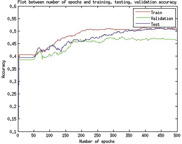
Figure 7 Plot of accuracy vs Number of epochs using max pooling.

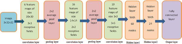
Figure 8 Best model for DCNN.

After applying convolution layer average pooling is applied for subsampling with a window size of 2 × 2. This 2 × 2 subsampling is results in 6 feature maps of size 15 × 15 and weights equal to 1/4 can be used.

Parameters:

Table 3 Parameters for model with best performance

Number of convolution layers	3
Number of pooling layers	3
Number of feature maps in convolutional layers	6, 20, 30
Receptive fields of convolutional layers	3 × 3, 2 × 2, 2 × 2 (overlapping)
Pooling/subsampling layer	Average Pooling in all the layers
Receptive Field of Pooling layers	2 × 2 (non-overlapping)
Activation function at fully connected layer	Tanh
No. of Hidden nodes in hidden layers	130, 80
No. of nodes in output layer	5 (5 classes)
Type of non-linearity	ReLU (Rectified Linear Units)
Loss Function	Mean Square Error
learning rate	0.001
optimization method	SGD (stochastic gradient descend)

Table 4 Task 1 – Confusion matrix

	Sheep	Car	Bus	Horse	Boat
Sheep	477	55	55	104	67
Car	49	924	60	2	7
Bus	58	90	655	89	82
Horse	3	0	15	732	0
Boat	57	5	62	3	900
Accuracy: 81.03%

Table 4 shows confusion matrix of DCNN classifier. It shows how different classes are being classified when a kernel size of 5 × 5 is used. From the confusion matrix it is clearly evident that can see the confusion between horse and sheep. Many of the sheep class data points are being classifiedas horse.

Task 2 – Classification of DCNN features using -SVM:

Extract the features using DCNN (from task 1) for the whole data set. Categorize the extracted data into train, test and validation data. Then train the SVM for different parameter values. Then the best model parameters are identified for SVM using cross validation method on validation data. Once we select the best model parameters for SVM, use those parameters on test data to get the accuracy of the model on test data. Gaussian kernel is used in this model as Gaussian kernel can better classify the data in the projected space according to the literature. Gaussian kernel on two data samples x₁, x₂ can be defined as:

K (x_{1}, x_{2}) = \frac{e^{- | | x_{1} - x_{2} | |}^{2}}{2 σ^{2}}

In C-SVM it is hard to set proper values for ‘C’ as there is no boundary on the values of ‘C’. In -SVM it is easy to set values for as can take values only within the range of 0 to 1 both inclusive. In our model > 0.5 values are infeasible. The best chosen parameters are = 0.5 and gamma = 0.03125.

Table 5 shows the confusion matrix of the SVM classifier. It shows how different classes are being classified when DCCN extracted features are classified using -SVM. From the confusion matrix it is clearly evident that majority of the sheep class data is misclassified. Many of the sheep class data points are being predicted as horse. We can see few misclassifications in the bus class too. It can be seen that for classes 2, 3 and 4 the performance is almost the same as DCNN. DCNN performs better on class1and SVM-with-DCNN works slightly better on class 5.

Table 5 Task 2 – Confusion matrix

	Sheep	Car	Bus	Horse	Boat
Sheep	465	58	66	105	64
Car	44	919	76	1	2
Bus	46	74	676	98	80
Horse	0	0	3	747	0
Boat	54	5	54	2	921
Accuracy: 81.75%

It is observed that performance of SVM is almost same or slightly better than using NN as classifier using DCNN features.

4 Conclusion

In the convolutional neural network designed, the number of feature maps in each convolutional layer and the number of pairs of convolutional and sampling layer define the complexity of the network. We have used average pooling and max pooling layer in our model and observed that for average pooling results in better performance than max pooling. We can infer that having several feature maps allow us to look for different patterns at different locations of the input image. If we increase the number of feature maps and convolutional layer beyond a limit, error on testing data starts increasing slowly. If we keep slightly high learning rate, after several iterations the training error go up presumably. The model can attain similar performance with considerably less feature maps just by adding two large fully connected hidden layers. We infer that number of units in fully connected hidden layer has as much impact as adding feature maps. As the weight for each feature map is the same it reduces the number of parameters to be estimated.

References

[1] Jyostna Devi Bodapati and N. Veeranjaneyulu, “Abnormal Network Traffic Detection Using Support Vector Data Description”, Proceedings of the 5th International Conference on Frontiers in Intelligent Computing: Theory and Applications. Springer, Singapore, 2017.

[2] Jyostna Devi Bodapati and N. Veeranjaneyulu, “Performance of different Classifiers in non-linear subspace” Proceedings of the International Conference on Signal and Information Processing, 2016.

[3] Veeranjaneyulu N and Jyostna devi Bodapati, “Scene classification using support vector machines with LDA”, Journal of theoretical and applied information technology, Vol. 63, pp. 741, 2014.

[4] Tara N. Sainath, Abdel-rahman Mohamed, Nrian Kingsbury, Bhuvana Ramabhadram, “Deep convolutional neural networks for LVCSR”, ICASSP, 2013.

[5] Alex Krizhevsky, Ilya Sutskever, Geoffrey E. Hinton, “Image Net Classification with Deep Convolutional Neural Networks”, NIPS, 2012.

[6] DH Hubel and TN Wiesel, “Receptive fields of single neurones in the cat’s striate cortex”, The Journal of Physiology, Vol. 3, pp. 574–579, 1959.

[7] LeCun, Yann, et al. “Gradient-based learning applied to document recognition”, Proceedings of the IEEE 86.11, pp. 2278–2324, 1998.

[8] Scherer, Dominik, Andreas Mller, and Sven Behnke, “Evaluation of pooling operations in Convolutional architectures for object recognition”, International Conference on Artificial Neural Networks, Springer Berlin Heidelberg, pp. 92–101, 2010.

[9] Krizhevsky, Alex, Ilya Sutskever, and Geoffrey E. Hinton, “Imagenet classiffication with deep convolutional neural networks”, Advances in neural information processing systems, 2012.

[10] Simon Haykin, “Neural Network and Learning Machines”, McMaster University Hamilton, Ontario, Canada.

[11] Zeiler, Matthew D., and Rob Fergus, “Stochastic pooling for regularization of deep convolutional neural networks”. arXiv preprint arXiv:1301.3557, 2013.

[12] Ikbal, M. Shajith, Hemant Misra, and Bayya Yegnanarayana, “Analysis of autoassociative mapping neural networks”, International Joint Conference Neural Networks, Vol. 5. IEEE, 1999.

[13] Jyostna devi Bodapati & N Veeranjaneyulu, “An Intelligent face recognition system using Wavelet Fusion of K-PCA, R-LDA”, ICCCCT, pp. 437–441, 2010.

[14] Ciregan, Dan, Ueli Meier, and Jürgen Schmidhuber. “Multi-column deep neural networks for image classification”. Computer vision and pattern recognition (CVPR), 2012 IEEE conference on. IEEE, 2012.

[15] Esteva, Andre, et al. “Dermatologist-level classification of skin cancer with deep neural networks”. Nature 542.7639, 2015.

[16] Courbariaux, Matthieu, Yoshua Bengio, and Jean-Pierre David. “Binaryconnect: Training deep neural networks with binary weights during propagations”. Advances in neural information processing systems, 2015.

[17] Cortes, Corinna, et al. “Adanet: Adaptive structural learning of artificial neural networks”. arXiv preprint arXiv:1607.01097, 2016.

[18] Shin, Hoo-Chang, et al. “Deep convolutional neural networks for computer-aided detection: CNN architectures, dataset characteristics and transfer learning”. IEEE transactions on medical imaging, 35.5, pp. 1285–1298, 2016.

[19] Toshev, Alexander, and Christian Szegedy. “Deeppose: Human pose estimation via deep neural networks”. Proceedings of the IEEE conference on computer vision and pattern recognition, 2014.

[20] Szegedy, Christian, Dumitru Erhan, and Alexander Toshkov Toshev. “Object detection using deep neural networks”. U.S. Patent No. 9,275,308, 2016.

[21] Neethu Narayanan, K. Suthendran and Fepslin AthishMon, “Recognizing Spontaneous Emotion From The Eye Region Under Different Head Poses”, International Journal of Pure and Applied Mathematics, Vol. 118, pp. 257–263, 2018.

Biographies

images

Jyostna Devi Bodapati working as Assistant Professor in the Department of Computer Science and Engineering, Vignan’s Foundation for Science, Technology and Research (Deemed to be University), Vadlamudi, India since 2010. She has published good number of research articles in reputed International journals and Conferences. Her areas of interests are Deep learning, Pattern Recognition and Kernel methods for pattern analysis.

images

N. Veeranjaneyulu is a Professor at Vignan’s Foundation for Science, Technology and Research (Deemed to be University), Vadlamudi, India. He has 21 years of teaching experience in the field of Computer Science. He has around 50 publications in International journals and Conference proceedings. His areas of interests are cloud computing and Big-data Analytics.