DDOS Detection on Internet of Things Using Unsupervised Algorithms

Victor Odumuyiwa^* and Rukayat Alabi

Department of Computer Science, University of Lagos, Nigeria

E-mail: vodumuyiwa@unilag.edu.ng; reykiaa@gmail.com

*Corresponding Author

Received 01 October 2020; Accepted 22 February 2021; Publication 25 May 2021

Abstract

The increase in the deployment of IOT networks has improved productivity of humans and organisations. However, IOT networks are increasingly becoming platforms for launching DDOS attacks due to inherent weaker security and resource-constrained nature of IOT devices. This paper focusses on detecting DDOS attack in IOT networks by classifying incoming network packets on the transport layer as either “Suspicious” or “Benign” using unsupervised machine learning algorithms. In this work, two deep learning algorithms and two clustering algorithms were independently trained for mitigating DDOS attacks. Emphasis was laid on exploitation based DDOS attacks which include Transmission Control Protocol SYN-Flood attacks and UDP-Lag attacks. Mirai, BASHLITE and CICDDOS2019 datasets were used in training the algorithms during the experimentation phase. The accuracy score and normalized-mutual-information score are used to quantify the classification performance of the four algorithms. Our results show that the autoencoder performed overall best with the highest accuracy across all the datasets.

Keywords: Distributed denial of service (DDOS), internet of things (IOT), machine learning algorithms, transmission control protocol (TCP), user datagram protocol (UDP), security.

1 Introduction

The increment of sensors and computing devices have made life easy and convenient for us due to the fast and accurate computation of our information. Nevertheless, the rapid increase in the deployment and combination of connected devices has truly expose essential resources to DDOS threats [1]. In 2016, the Mirai attack that ruined several notable websites actually exposed the weakness of IOT devices [2]. Over 100,000 inadequately protected player, cameras, digital video recording and other IOT devices were turned into botnets. The Mirai source code that was further released resulted in frequent additional IOT attacks. With the magnitude of attacks that have been launched, securing IOT devices is a problem as host-centric IT security solutions cannot be totally relied upon because most manufacturers appliances place more priority on functionality and cost over security. Besides, unlike servers that can undergo software update, IOT software is hardly or never updated, hence making them more vulnerable to attackers. In view of these security problems and resource-constrained nature of IOT devices, greater focus should be placed on packet security within the IOT network.

Traditional network-centered security has relied on predefined signature or system representations for known threats [3]. Recently, the awareness of using machine learning to secure network has increased rapidly. However, many of the machine learning solutions use supervised learning i.e. they create attack classifiers by training on identified anomalies [4], which makes them futile towards new threats. The main aim of this work is to determine the performance of unsupervised learning algorithms in accurately classifying network packets as either benign or malicious. We achieve this by training the algorithms on modern DDOS datasets and performing rigorous testing while benchmarking the performance of the algorithms using standard performance metrics.

The rest of the paper is organized as follows: Section 2 presents related works; Section 3 elaborates the data set and describes the methodology followed in the research; Section 4 details the experimentation procedures, the result gotten and the observations from the results while Section 5 discusses the conclusion of our research as well as highlighting the future work.

2 Related Work

According to [5], detection systems of network intrusion have traditionally been rule-based. Nevertheless, machine learning and statistical approaches have also made major contributions [5]. Machine learning have also proven to be effective in two main ways of securing network which are: feature engineering (i.e. ability to extract the most important structures from network data to assist model learning) [6] and classification. In security environment, classification tasks usually involve training both suspicious and benign data to build models that can detect known attacks [7].

The authors in [8] pointed out that steps such as collection of network information, feature extraction and analysis, and classification detection provide a means for building efficient software-based tools that can detect anomalies such as software-defined networking (SDN). Another study [9] provides a thorough classification of DDOS attacks in terms of detection technology. The study also emphasizes how the characteristics of the network security of an SDN defines the possible approaches to setting up a defense against DDOS attacks. Similarly, [10] have explored this area too. In other approaches to DDOS defense, [4] propose a scheduling based SDN controller architecture to effectively limit attacks and protect networks in DoS attacks.

The growth of cloud computing and IOT has inevitably led to the migration of denial-of-service attacks on cloud computing devices as well. Thus, cloud computing devices must implement efficient DDOS detection systems in order to avoid loss of control and breach of security [11]. Studies such as [12] aimed at tackling this problem by determining the source of a DDOS attack using PTrace (powerful trace) source control methods. PTrace controlled such attack sources from two aspects, packet filtering and malware tracing, to prevent the cloud from becoming a tool for DDOS attacks. Other studies such as [13] approach the problem of filtering by using a set of security services called filter trees. In the study, XML and HTTP based DDOS attacks are filtered out using five filters for detection and resolution. Detection based on classification has also been proposed and a classifier system for detection against DDOS TCP flooding attacks was created [14]. These classifiers work by taking in an incoming packet as input and then classifying the packet as either suspicious or otherwise. The nature of an IP network is often susceptible to changes such as the flow rate on the network and in order to deal with such changes, self-learning systems have been proposed that learn to detect and adapt to such changes in the network [15].

Many of the existing models for DDOS detection have primarily focused on SYN-flood attacks and haven’t been trained to detect botnet attributes. More studies are thus needed where models are trained to detect botnet as botnet becomes the main technology for DDOS organization and execution [16]. Botnet DDOS attacks infect multitude of remote systems turning them to zombie nodes that are then used for distributed attacks. In detecting botnet DDOS attacks, authors in [17] used a deep learning algorithm to detect TCP, UDP and ICMP DDOS attacks. They also distinguished real traffic from DDOS attacks, and conducted an in-depth training on the algorithm by using real cases generated by existing popular DDOS tools and DDOS attack modes. Also, [18] proposed a DDOS attack model and demonstrated that by modelling different allocation strategies, the proposed DDOS attack model is applicable to game planning strategies and can simulate different botnet attack characteristics.

According to [19], DDOS detection approaches can operate in one of the following three modes: supervised, semi-supervised and unsupervised mode. For the detection approach in supervised mode, it requires a trained model (or a classifier) to detect the anomalies, where the dataset for training includes input variables and output classes. The trained model is used to get the hidden functions and predict the class of input variables (incoming traffic instances). This is consider as classification under supervised data mining [20]. For the approaches that work in the semi-supervised mode, they have incomplete training data i.e. training data is only meant for normal class and some targets are missing for anomaly class [21]. Unlike supervised and semi-supervised learning, unsupervised machine learning algorithms do not have any input-output pairs but the algorithm is trained such that it can accurately determine the unknown data point. The following subsections further discusses the unsupervised learning algorithms we used in this work.

3 Methodology

A DDOS attack temporarily or indefinitely constraints the availability of a network resource to its intended users. The challenge then for the network administrator is to deploy DDOS detection systems that are capable of analysing incoming packets to the transport layer. These detection systems may then determine if these incoming packets are suspicious or benign. In the following subsections, we present the design methodology for a DDOS detection system that uses unsupervised machine learning algorithms. The problem is therefore to design and train four efficient unsupervised machine learning systems that are capable of detecting a DDOS attack on the transport layer.

3.1 Datasets

In order to train the unsupervised machine learning algorithms, the following DDOS attack datasets were sourced.

1. The first dataset is the DDOS evaluation dataset (CICDDOS2019) [27]. The full dataset consists of both reflection and exploitation based DDOS attacks in the form of both suspicious and benign network packets. The dataset is further grouped into TCP and UDP based attacks.

2. The second dataset is the Mirai dataset created by [28]. Mirai is a specific type of botnet malware that overrides networked Linux devices and successfully turns them into bots used for distributed attacks such as DDOS. The Mirai dataset consists of 80,000 SYN-flood instances and 65,000 UDP-lag attacks on security camera IOT devices.

3. Finally, the third dataset is the BASHLITE botnet attack dataset on a webcam IOT device and is also provided by [28]. Similar to Mirai, BASHLITE is a botnet malware for distributed attacks on networked devices. The BASHLITE dataset consists of 110,000 SYN-flood instances and 100,000 UDP-lag attacks. Both Mirai and BASHLITE are open-source malware that can be used for academic research purposes.

3.2 Data Preprocessing

The dataset largely consists of numerical values, so the preprocessing steps are minimal. The most important preprocessing action taken was to normalize the values in the dataset using the standard minmax normalization expressed below in Equation (1).

x^{'} = \frac{x - m i n (x)}{m a x (x) - m i n (x)}

(1)

3.3 Selected Unsupervised Learning Algorithms

The selected unsupervised machine learning algorithms employed in this work are explained below.

3.3.1 Autoencoder (AE)

According to [6], Autoencoders can be defined as a neural network that detect a similar function that is used to reconstruct the input data with high accuracy by using back propagation. The Autoencoder has two main fragments (cf. Figure 1), “an encoder that compresses the input into a dimensional latent subspace that is lower and a decoder that recreate the input from this latent subspace”. The encoder and the decoder, can be defined as transitions $ϕ$ and $ψ$ such that:

$ϕ : X \to F$
$ψ : F \to X$
$ϕ, ψ = argmin ϕ, ψ {∥ X - (ψ \circ ϕ) X ∥}^{2}$	(2)

The autoencoder is made up of two feed forward neural networks that mirror each other in terms of the number of layers and the number of nodes. The goal of the autoencoder model is to learn the latent space of an encoded vector that can be used to efficiently reconstruct the input vector. Thus, the goal of the encoder is to encode the input vector to a lower dimensional vector space [3]. The goal of the decoder is to reconstruct this input vector from the lower dimensional encoded vector provided by the encoder. Figure 1 shows the architecture for our autoencoder model, it can be seen that the input vector is structured with respect to the 77 features from the CICDDOS2019 dataset. We simply increase this number to 115 when working with the Mirai and BASHLITE datasets, all other parameters stay the same.

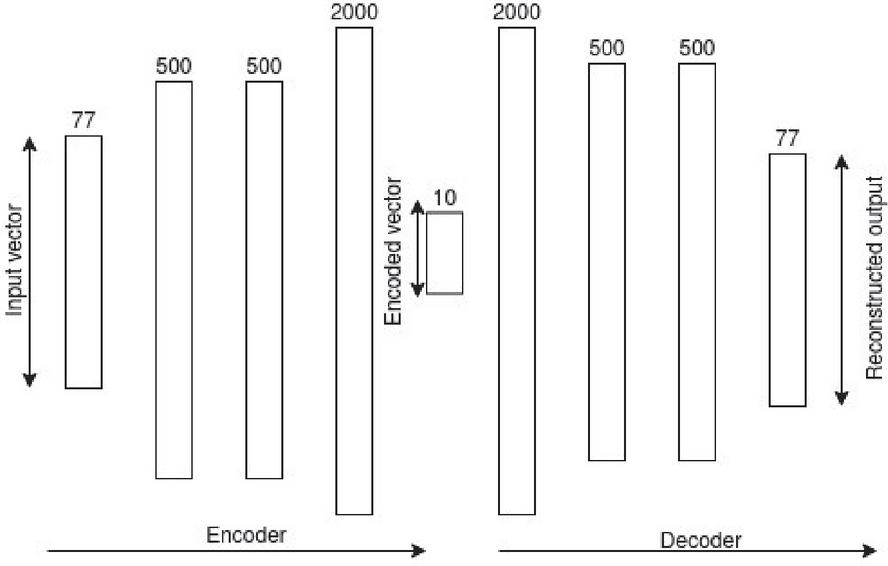
Figure 1 The Autoencoder architecture.

Each neuron in the hidden layers of the encoder and decoder make use of the Rectified Linear Unit (ReLu) activation function. The hyperparameters selected for the autoencoder model are outlined as follows;

• Batch size: A batch size of 2048 is selected.

• Number of epochs: An epoch number ranging between 10–20 is initialized.

• Loss: The mean squared error loss function is used.

• Optimizer: Adam, an adaptive algorithm, is selected. It is a state-of-the-art optimizer for deep neural networks (Schneider et al, 2019).

• Betas: These are Adam optimizer coefficients used for computing running averages of gradient and its square (0.5, 0.999).

• Learning rate (0.0002).

3.3.2 Restricted Boltzmann machine (RBM)

The restricted Boltzmann machine is a generative model that is used to sample and generate instances from a learned probability distribution. Given the training data, the goal of the RBM is to learn the probability distribution that best fits the training data. The RBM consists of $m$ visible units $V = (V_{1}, V_{2} \dots, V_{m})$ and $n$ hidden units $H = (H_{1}, H_{2} \dots, H_{n})$ arranged in two layers.

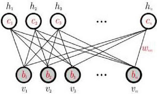
Figure 2 Restricted Boltzmann machine showing the visible and hidden units.

The visible units lie on the first layer and represent the features in the training data (see Figure 2). Usually, one visible unit will represent one feature in an example in the training data. The hidden units model and represent the relationship between the features in the training data. The random variables $(V, H)$ take on values $(v, h) \in {[0, 1]}^{m}$ for continuous variables and the underlying probability distribution in the training data is given by the Gibbs distribution $p (v, h) = 1 / z^{- E (v, h)}$ with the energy function in Equation (3);

E (v, h) = - \sum_{m}^{n} \sum_{m}^{n} w_{ij} v_{i} h_{j} - \sum_{i = 1}^{m} b_{i} v_{i} - \sum_{j = 1}^{n} c_{j} h_{j}

(3)

In Equation (3), $w_{ij}$ are real valued weights associated with $v_{j}$ and $h_{i}$ , and $b_{j}$ and $c_{i}$ are real valued bias terms associated with units $i$ and $j$ respectively. The contrastive divergence learning algorithm is one of the successful training algorithms used to approximate the log-likelihood energy gradient and perform gradient ascent to maximize the likelihood [24].

The RBM used for this project is a two-layer RBM with an architecture as described in Figure 2. The dataset consists of continuous variables scaled between 0 and 1 so therefore we model the RBM as a continuous variable model with the hidden units and visible units taking on values between $(v, h) \in {[0, 1]}^{m}$ where $m$ is number of visible units. Similar to the autoencoder algorithm, we use the reconstruction error to define the classification task for the RBM. The parameters selected for the RBM include:

• Number of units: The number of hidden and visible units are set to be the same value according to the number of features present in the training data. That is, for instance for the CICDDOS2019, the number of hidden and visible units for the RBM is 77.

• Training algorithm: The k-step contrastive divergence algorithm with Gibbs sampling is used for training the algorithm with $k = 10$ .

• Training Epoch: An epoch of 10 is selected, experimental results show that increasing the epoch beyond 10 does not improve training results.

3.3.3 K-Means

The K-means algorithm takes the full dataset consisting of multiclass data points, then clusters the datapoints into separate clusters to the best of its ability; this classification occurs when you feed in the input and the model assigns the input into one of the computed clusters. Assumed a set of observations ( $x_{1}$ , $x_{2}$ , $x_{3}, \dots$ , $x_{n}$ ), where each observation is a d-dimensional real vector, the k-means objectives is to partition the n observations into k ( $\leq$ n) sets $S = {s_{1}, s_{2}, \dots, s_{k}}$ in order to reduce the within-cluster sum of squares (WCSS) (i.e. variance).

The K-Means clustering algorithm has relatively fewer parameters to select. The default “pure” version of the K-means algorithm is used as opposed to variants such as Elkan’s K-Means [29] where triangle inequality is used. The parameters for the algorithm are outlined as follows;

• Number of clusters: This is the number of clusters as well as the number of centroids to generate. Two (2) clusters are required since we will be attempting to classify and thus cluster suspicious or benign samples.

• Number of initializations: This is the number of times the algorithm will be run with different centroid seeds. We have the option of 20 initializations depending on the performance.

• Precompute distance: Here the algorithm precomputes the distance between sample points in the feature space. Enabling this parameter allows the algorithm to train faster.

3.3.4 Expectation-Maximization (EM)

The authors in [25] stated that EM algorithm is used for solving mixture models that assume the existence of some unobserved data. Mathematically, the EM algorithm can be described as follows; “given the statistical model that generates a set of observed data $X$ , latent data $Z$ ,” unknown parameters $θ$ and the likelihood function $L (θ; X) = p (X, Z | θ)$ , the maximum likelihood of the unknown data $θ$ is determined by maximizing the marginal log-likelihood of the observed data $X$ using Equation (4):

L (θ; X) = p (X | θ) = \int p (X, Z | θ) d Z

(4)

The expectation and maximization steps are defined as follows:

$Q (θ \| θ^{(t)})$	$= E_{Z \| X, θ^{(t)}} [\log L (θ, X, Z)]$	(5)
$θ^{t + 1}$	$= a r g m a x_{θ} Q (θ \| θ^{(t)})$	(6)

In the expectation step, the likelihood of the unknown parameters is computed as the log-likelihood of the known parameter estimates, while in Equation (5) the maximization step is used to select the new value that maximizes the log-likelihood given the estimates from Equation (6).

The expectation-maximization algorithm is setup with similar parameters as the k-means algorithm and in fact the software implementation of the two algorithms in the sci-kit learn machine learning framework borrow from each other. However, the core implementations are different from studies such as [22, 26] and the parameters for the expectation maximization algorithm include:

• Number of components: This is the number of clusters to be estimated and is set to two because of the binary classification task of suspicious or benign.

• Number of iterations: The number of iterations is like the epoch of the autoencoder where they both define the number of training iterations to run the algorithm. A default value of 300 is used.

• Covariance type: The covariance parameter defines the structure of the covariance matrix with respect to each component or cluster. The “full” covariance is chosen where each cluster has its own covariance matrix and has been shown to achieve the best results.

3.4 Evaluating Model Performance

3.4.1 Accuracy

In machine learning parlance, the task of determining whether or not an incoming packet is suspicious or benign is known as classification. For the K-Means and EM algorithm, the clustering of a feature point together with highly similar feature points is in itself, a form of classification. We can evaluate these models by quantifying how accurate their classification of a packet is with respect to its clusters. A simple net accuracy score of the predicted class compared to the actual class gives us an empirical quantification of the model’s performance.

For the autoencoder and Boltzmann model, this classification task is non-trivial. This is because, these algorithms are not clustering algorithm like the K-Means model and neither do they output a single value classification like the feed forward neural network with one output neuron. We approach the problem from the viewpoint of the properties of the autoencoder and restricted Boltzmann machine [30] (Bhatia et al., 2019). Since the optimal performance of the deep learning models is such that the reconstructed output vector must be very similar to the original input vector (see Figure 3.3), the autoencoder will have learnt to reconstruct a very specific domain of feature points. We can define a reconstruction error that describes the difference between the reconstructed output and original input vector. The reconstruction error is defined as the mean squared error (MSE) in Equation (7) as follows:

M S E = \frac{1}{n} \sum_{i = 1}^{n} {(y_{i} - {\hat{y}}_{i})}^{2}

(7)

Where $y_{i}$ is the original input vector and ${\hat{y}}_{i}$ is the reconstructed output vector. The mean squared error is computed over all the output of the model. Ideally, it is preferable to have a mean squared error close to zero. However, depending on the size of the values in the predicted output, a mean squared error within the range of 2–5 decimal places is acceptable. Representing the reconstruction error as the mean squared error allows one to know when the model is presented with an input that is very far off from what was contained in the training set. Thus, if for instance the autoencoder is trained on a dataset comprising only of benign packets, whenever a benign packet is presented to the autoencoder, we expect that the reconstructed output should be quite similar and therefore the reconstruction error should be low. However, if this same model is presented with a suspicious packet that is fairly different from the features of benign packet then we should expect the reconstruction error to be quite high. The same logic can be applied to the restricted Boltzmann machine.

With this formulation established, it is easier to frame the classification problem using the autoencoder and RBM. Where in our example, a low reconstruction error means the packet is benign, while a high reconstruction error means the packet is suspicious. Using these predictions, we can then compute the accuracy much like we did with the K-Means model. The accuracy score simply calculates a ratio of the number of correctly classified packets over the incorrectly classified packets.

3.4.2 Normalized mutual information (NMI)

The NMI provides a means of evaluating the clustering performance of the algorithm by comparing the correlation between the predicted class and the target class. If the predicted and target data are represented as two separate distributions, then we can also apply the NMI to determine performance of non-clustering algorithms. Therefore, we can apply the NMI metric to the classification performance of the autoencoder and RBM too. The Normalized mutual information is scaled between 0 and 1. Where 1 represents perfect correlation and 0 otherwise. In general, a higher NMI above 0 is preferable. The exact interpretations of the NMI alone may not be sufficient to quantify the model’s performance that is why the concept of accuracy is also reviewed. This is because the NMI is a statistical property that describes correlation between two distributions [31]. A high NMI does not necessarily translate to a higher accuracy and vice versa. Thus, the two metrics should be regarded independently.

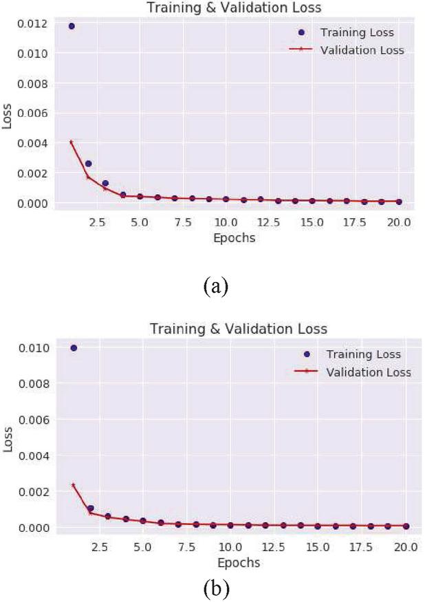
Figure 3 Autoencoder training and validation loss on the CICDDOS2019 SYN-Flood (a) and UDP-Lag (b).

4 Experimental Results

In this session, we present the experimental results for each model across all datasets. The results are presented in subsections, with each subsection dedicated to a model. For the Autoencoder and Restricted Boltzmann Machine, their subsections consist of plots showing the training and test loss, a table summarizing the performance across the datasets and a detailed discussion of the results. For the rest of the models, they do not optimize a loss function and so only the summary tables and a detailed discussion of the results were presented. Performance evaluations are also carried out using the accuracy and Normalized Mutual score. Tables 5 and 6 also show the summary of all the results of the different models.

4.1 Autoencoder training and test results

Figure 3 shows the desired behaviour of the backpropagation training algorithm where the training and validation loss decrease steadily and in unison as the training epoch increases. It is important to point out that the autoencoder is trained to reconstruct SYN-Flood data, meaning it should be unable to reconstruct benign data. We chose the SYN-Flood data for training because there were more instances than the benign data. The same choice is made for the UDP-Autoencoder model, where we train it on the UDP-Lag data instead of on benign UDP data.

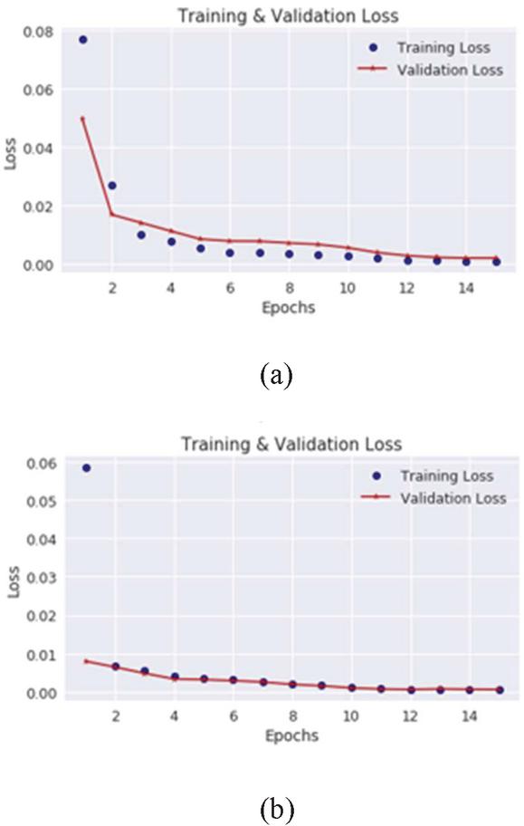
Figure 4 Autoencoder training and validation loss on the Mirai SYN-flood (a) and UDP-Lag data (b).

In Figure 4(a) and 4(b), the training and validation loss of the Autoencoder model on the Mirai SYN and UDP-Lag data reduces steadily as the training epochs increase. It is clear that by epoch 10, the loss starts to converge quickly to zero. Therefore 20 is the sufficient number of training epochs in order to avoid overfitting.

The training and validation loss for the BASHLITE loss shown in Figure 5 is less steep than that of the Mirai loss. Table 1 shows the accuracy of the autoencoder model across all datasets, here we can see that the model has the highest accuracy on the BASHLITE dataset hence the reason why the loss is less steep and flattens out quickly by epoch 10 and 14 respectively.

In Table 1, we present the accuracy and NMI scores for the autoencoder model. These scores were determined based on the formulation described in Section 3.4. The result show that the autoencoder model performs best on the BASHLITE SYN-Flood data with a higher accuracy of 99%. In general, the autoencoder performs better on the Mirai and BASHLITE datasets than that of the CICDDOS2019 dataset. Does this mean the model is better suited to detect botnet attacks? We suspect that this is due to the feature selection process for the datasets, the Mirai and BASHLITE datasets show less variance across the features when compared to the CICDDOS2019 dataset. The NMI scores show higher correlations where the accuracy is higher, indicating a correlation between the target predictions and predicted value.

4.2 Restricted Boltzmann Machine

The restricted Boltzmann machine performed poorly on the CICDDOS2019 dataset but the training process evolved smoothly with the loss dropping as the epoch increased (Figure 6). The RBM loss did not drop as low as that of the autoencoder loss for the CICDDOS2019.

Table 1 Test Accuracy and Normalized Mutual Information score for the autoencoder models on the SYN-Flood and UDP-Lag across all datasets

Data	Accuracy (%)	NMI
CICDDOS2019 SYN-Flood	0.8945	0.5363
CICDDOS2019 UDP-Lag	0.8617	0.4216
Mirai SYN-Flood	0.9744	0.6211
Mirai UDP-Lag	0.9621	0.5733
BASHLITE SYN-Flood	0.9933	0.9927
BASHLITE UDP-Lag	0.9921	0.9822

Also, the training procedure and implementation of the RBM did not enable us to run a training and validation set simultaneously as we did with the autoencoder. Thus, the training loss is presented only.

Figure 5 Autoencoder training and validation loss on the BASHLITE SYN-flood (a) and UDP-Lag data (b).

Oscillations in the training loss were observed during the training of the RBM on the Mirai dataset. Such oscillations are quite common in training of generative models using batch sampling because the batch sampling prevents the loss function from settling in a local optimum. The oscillations in the loss indicate that the training algorithm continues to explore the search space not settling for a local optimum. The test set results of the RBM on the Mirai dataset show improvement over the CICDDOS2019 dataset with its highest accuracy score being recorded against the Mirai UDP-Lag (Table 2).

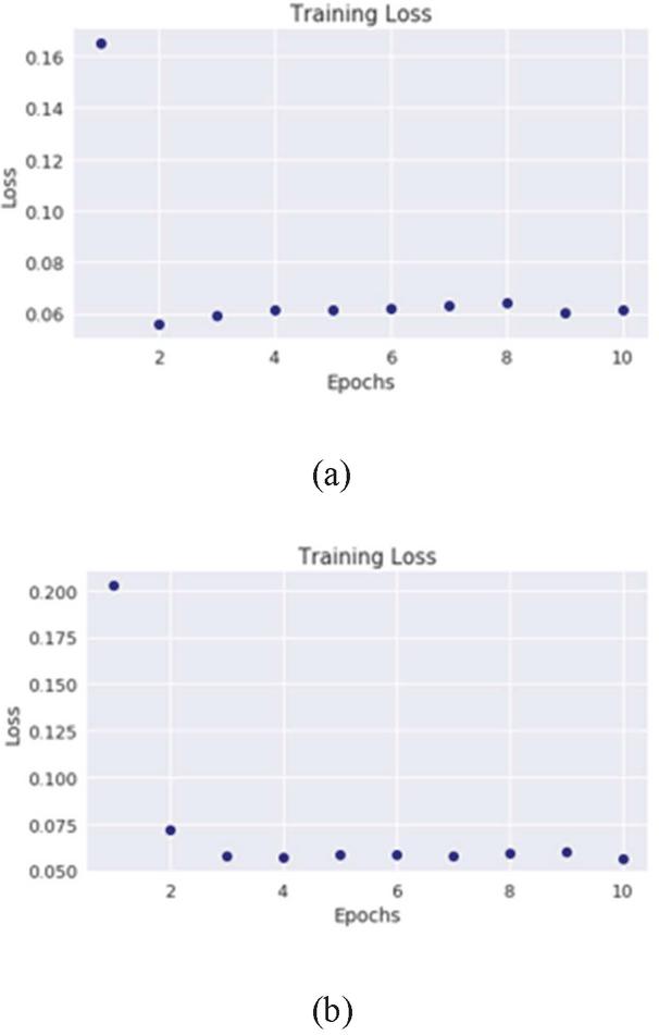
Figure 6 Restricted Boltzmann machine training loss on the CICDDOS2019 SYN-flood (a) and UDP-Lag data (b).

Table 2 Test Accuracy and Normalized Mutual Information score for the Restricted Boltzmann machine model on the SYN-Flood and UDP-Lag across all datasets

Data	Accuracy (%)	NMI
CICDDOS2019 SYN-Flood	0.5651	0.1919
CICDDOS2019 UDP-Lag	0.5089	0.1103
Mirai SYN-Flood	0.6067	0.1639
Mirai UDP-Lag	0.7797	0.3895
BASHLITE SYN-Flood	0.6709	0.2506
BASHLITE UDP-Lag	0.6210	0.1007

The RBMs performance on the BASHLITE dataset is similar to its performance on the Mirai data, still, the overall performance is much lower than that of the Autoencoder. The results indicate that the RBM is less suited for the kind of precise reconstruction of the continuous input value that is easily achieved by the autoencoder. The stochastic property of the RBMs hidden units makes it difficult to accurately reconstruct the continuous input from a large unknown latent space. The autoencoder solves this problem by first encoding the input vector into a lower dimensional space thus reducing the dimensionality of the latent space, making the resampling process more accurate and less computationally intensive. The NMI across the RBMs performance is low, showing poor correlation between the target and predicted value.

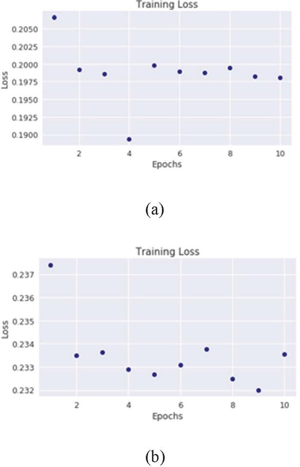
Figure 7 Restricted Boltzmann machine training loss on the Mirai SYN-flood (a) and UDP-Lag data (b).

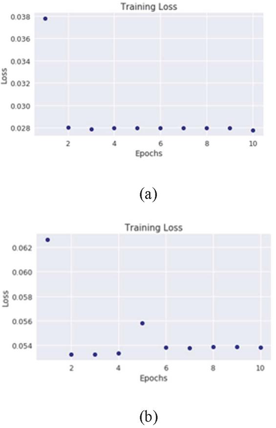
Figure 8 Restricted Boltzmann machine training loss on the BASHLITE SYN-flood and UDP-Lag data.

4.3 K-Means Training and Test Results

The K-Means algorithm is not a gradient based learner so we cannot bother ourselves with iterative plots such as those presented for the autoencoder and RBM models. Also, the K-Means algorithm is trained on a distribution that contains a mixture of both suspicious and benign features. The model’s accuracy and NMI are shown in Table 3.

Table 3 Test Accuracy and Normalized Mutual Information score for the K-Means model on the SYN-Flood and UDP-Lag training and validation data

Data	Accuracy (%)	NMI
CICDDOS2019 SYN-Flood	0.7538	0.1949
CICDDOS2019 UDP-Lag	0.7139	0.1427
Mirai SYN-Flood	0.7636	0.0912
Mirai UDP-Lag	0.7478	0.1387
BASHLITE SYN-Flood	0.6451	0.1059
BASHLITE UDP-Lag	0.6823	0.1306

From the results, we observe that the K-Means model performs relatively poorer as compared to the autoencoder model but it performs better on average when compared to RBM. However, and once again, one can see some slight disparity in performance on the SYN-Flood data compared to UDP-Lag data owing to the variance amongst the features in these datasets.

The NMI scores for the K-Means model are relatively low too with well below average correlations. Although one should interpret the accuracy and NMI scores independently, the low NMI scores for the K-Means discourages one from being too optimistic about the model’s performance.

4.4 Expectation-Maximization Training and Test Results

The Expectation-Maximization algorithm performs better than the k-means algorithm on average with its highest accuracy being 80% on the Mirai UDP-lag data (Table 4).

Table 4 Test Accuracy and Normalized Mutual Information score for the EM model on the SYN-Flood and UDP-Lag training and validation data

Data	Accuracy (%)	NMI
CICDDOS2019 SYN-Flood	0.7096	0.1144
CICDDOS2019 UDP-Lag	0.6759	0.1446
Mirai SYN-Flood	0.7030	0.2771
Mirai UDP-Lag	0.8051	0.2901
BASHLITE SYN-Flood	0.7636	0.3074
BASHLITE UDP-Lag	0.7575	0.2678

Although, the EM algorithm performs better than the k-means algorithm the performance is still poor compared to the autoencoder. The clustering algorithms struggle with large high-dimensional and continuous data. The maximization step in the EM algorithm gives it an edge over the k-means algorithm in this aspect. Where the k-means algorithm struggles to compute a centroid from high dimensional continuous data, with low variance as is the case with Mirai and BASHLITE, the EM algorithm models the problem probabilistically instead, optimizing for the log-likelihood of the latent variables.

Tables 5 and 6 above summarize the accuracy and NMI scores across all datasets for all models, highlighting the autoencoder’s superiority for machine learning task.

Table 5 Summary of the Accuracies across all datasets and all models

Dataset/		Restricted		Expectation-
Model	Autoencoder	Boltzmann Machine		Maximization
CICDDOS2019 SYN-Flood	0.8945	0.5651	0.7538	0.7096
CICDDOS2019 UDP-Lag	0.8617	0.5089	0.7139	0.6759
Mirai SYN-Flood	0.9744	0.6067	0.7636	0.7030
Mirai UDP-Lag	0.9621	0.7797	0.7478	0.8051
BASHLITE SYN-Flood	0.9933	0.6709	0.6451	0.7636
BASHLITE UDP-Lag	0.9921	0.6210	0.6823	0.7575

Table 6 Summary of the Normalized Mutual Information score across all datasets and all models

Dataset/		Restricted		Expectation-
Model	Autoencoder	Boltzmann Machine		Maximization
CICDDOS2019 SYN-Flood	0.5363	0.1919	0.1949	0.1144
CICDDOS2019 UDP-Lag	0.4216	0.1103	0.1427	0.1446
Mirai SYN-Flood	0.6211	0.1639	0.0912	0.2771
Mirai UDP-Lag	0.5733	0.3895	0.1387	0.2901
BASHLITE SYN-Flood	0.9927	0.2506	0.1059	0.3074
BASHLITE UDP-Lag	0.9822	0.1007	0.1306	0.2678

5 Conclusion

The unsupervised machine learning models were trained on both SYN-Flood and UDP-Lag DDOS datasets. The training and test results both show that the deep learning autoencoder model performs better in the classification of incoming packets as suspicious or benign. Over the past decade, deep learning algorithms have established themselves as the state-of-the-art machine learning algorithms. Our results show that in the unsupervised machine learning space, the deep learning algorithm also outperforms traditional clustering algorithms such as the K-Means and Expectation-Maximization algorithm as well as other generative deep learning models such as the Restricted Boltzmann machine. However, when comparing unsupervised machine learning algorithms, one must be careful to formalize the performance evaluation problem properly. This work shows that it is possible to frame the autoencoder model as a classification algorithm using the value of the reconstruction error and that it is possible to apply this formulation efficiently to difficult problem domains such as network packet analysis. Once proper formulations are established, the accuracy score can then be used to evaluate both models fairly. Although the autoencoder model is clearly the superior model, the DDOS-Detection tool we developed provides methods that allow one to perform network packet classification using either the autoencoder model or the Expectation-Maximization model. The simulation results show that the DDOS-Detection tool built around these models can achieve a net accuracy of as high as 99%. Future studies should aim to replicate results in a larger system to detect compromised end-points and carry out possible retraining of the models with recent data to handle abnormalities in network performance.

References

[1] Shirazi, “Evaluation of anomaly detection techniques for scada communication resilience,” IEEE Resilience Week, 2016.

[2] N. Mirai, “mirai-botnet,” 2016. [Online]. Available: https://www.cyber.nj.gov/threat-profiles/botnetvariants/mirai-botnet. [Accessed 31 December 2019].

[3] H. Zhou, B. Liu and D. Wang, “Design and research of urban intelligent transportation system based on the Internet of Things,” Internet of Things, pp. 572–580, 2012.

[4] S. Lim, S. Yang and Y. Kim, “Controller scheduling for continued SDN operation under DDOS attacks,” Electronic Letter, pp. 1259–1261, 2015.

[5] A. Buczak and E. Guven, “A survey of data mining and machine learning methods for cyber security intrusion detection,” IEEE Communications Surveys & Tutorials, vol. 18.2, 2016.

[6] P. Baldi, “Autoencoders, Unsupervised Learning, and Deep Architectures,” Proceedings of ICML workshop on unsupervised and transfer learning, 2012.

[7] R. Doshi, N. Apthorpe and N. Feamster, “Machine Learning DDOS Detection for Consumer Internet of Things Devices,” IEEE Deep Learning and Security Workshop, 2018.

[8] Q. Yan, F. Yu and Q. Gong, “Sotware defined networking and Distributed denial of service attacks in cloud computing environments,” IEEE Communications Survey & Tutorial, no. 18, pp. 602–622, 2016.

[9] N. Z. Bawany, J. A. Shamsi and K. Salah, “DDOS Attack Detection and Mitigation Using SDN,” Arabian Journal for Science & Engineering, no. 2, pp. 1–19, 2017.

[10] B. Kang and H. Choo, “An SDN-enhanced load-balancing technique in the cloud system[J].,” Journal of Supercomputing, pp. 1–24, 2016.

[11] O. Osanaiye and D. M. Choo, “Distributed denial of service (DDOS) resilience in cloud,” Journal of Network & Computer Applications, pp. 147–165, 2016.

[12] H. Luo, Z. Chen and J. Li, “Preventing Distributed Denial-of-Service Flooding Attacks With Dynamic Path Identifiers[J],” IEEE Transactions on Information Forensics & Security, pp. 1801–1815, 2017.

[13] U. Dick and T. Scheffer, “Learning to control a structured-prediction decoder for detection of HTTP-layer DDOS attackers,” in Machine Learning, 2016, pp. 1–26.

[14] Z. Gao and N. Ansari, “Differentiating Malicious DDOS Attack Traffic from Normal TCP Flows by Proactive Tests[J],” Communications Letters IEEE, pp. 793–795, 2006.

[15] K. Borisenko, A. Rukavitsyn and A. Gurtov, “Detecting the Origin of DDOS Attacks in OpenStack Cloud Platform Using Data Mining Techniques[M]// Internet of Things,” Smart Spaces, and Next Generation Networks and Systems, 2016.

[16] N. Hoque, D. Bhattacharyya and J. Kalita, “Botnet in DDOS Attacks: Trends and Challenges[J],” IEEE Communications Surveys & Tutorials, pp. 1–1, 2015.

[17] A. Saeed, R. E. Overill and T. Radzik, “Detection of known and unknown DDOS attacks using Artificial Neural Networks,” Neurocomputing, pp. 385–393, 2016.

[18] S. Ramanauskaite, N. Goranin and A. Cenys, “Modelling influence of Botnet features on effectiveness of DDOS attacks[J],” Security & Communication Networks, pp. 2090–2101, 2015.

[19] C. Buragohain, M. J. Kaita, S. Singh and D. K. Bhattacharyya, “Anomaly based DDOS attack detection,” International Journal of Computer Applications, pp. 35–40, 2015.

[20] A. Aggarwal and A. Gupta, “Survey on data mining and IP traceback technique in DDOS attack,” International Journal of Engineering and computer science, vol. 4(6), pp. 12595–12598, 2015.

[21] G. Nadiammai and M. Hemalatha, “Effective approach towards intrusion detection system using data mining technique,” Egyptian Informatics Journal, vol. 15(1), pp. 37–50, 2014.

[22] Y. A. Mahmood, “Autoencoder-based feature learning for cybersecurity applications,” International Joint Conference on Neural Networks (IJCNN), 2017.

[23] S. Yadav and S. Subramanian, “Detection of Application Layer DDOS attack by feature learning using Stacked AutoEncoder,” International Conference on Computational Techniques in Information and Communication Technologies (ICCTICT), 2016.

[24] A. Fischer and C. Igel, “An introduction to restricted Boltzmann machines. In Ibero American congress on pattern recognition,” Springer, Berlin, Heidelberg, pp. 14–36, 2012.

[25] V. G. Ryzin and G. Vulcano, “An expectation maximization method to estimate a rank-based,” 2017.

[26] D. Ferreiraetal, “Extreme Dimensionality Reduction for Network Attack Visualization with Autoencoders,” International Joint Conference on Neural Networks (IJCNN), 2019.

[27] I. Sharafaldin, A. H. Lashkari, S. Hakak and A. Ghorbani, “Developing Realistic Distributed Denial of Service (DDOS) Attack Dataset and Taxonomy,” International camahan conference on security (ICCST). IEEE, pp. 1–8, 2019.

[28] Y. Meidan, M. Bohadana, Y. Mathov, Y. Mirsky and Shabtai, “Network based detection of IOT botnet attacks using deep autoencoders,” IEEE Pervasive Computing, pp. 12–22, 17(3).

[29] C. Elkan, “Using the triangle inequality to accelerate k-means,” ICML-03, pp. 147–153, 2003.

[30] B. Barricelli and E. Casiraghi, “A Survey on Digital Twin: Definitions, Characteristics, Applications, and Design Implication,” IEEE Acces, vol. 7, pp. 167653–167671, 2019.

Biographies

Victor Odumuyiwa obtained his Ph.D. in 2010 from Nancy 2 University in France. He was an ETT fellow at the Massachusetts Institute of Technology, Boston, USA in 2013. He is a certified security intelligence analyst and application security analyst. He is also a member of the Global EPIC eco-system centred on innovation and cyber security. His research centres on Web Intelligence and Cyber Security. He is a Senior Lecturer at the Department of Computer Science, University of Lagos, Nigeria.

Rukayat Alabi is a business analyst and also an aspiring Ph.D. student in Computer science. She was part of the team that developed the pensioner automated system used currently in Nigeria. She is certified in the following: MCSA, ITIL, MOS Master, MCE and IC3. Her research area currently covers security in internet of things and positive impacts of technology in business.