Konstantinos Maliatsos, Panagiotis N. Vasileiou and Athanasios G. Kanatas

• Department of Digital Systems, University of Piraeus, Greece, kmaliat;panvas;kanatas@unipi.gr

Abstract

Beamspace MIMO (BS-MIMO) systems have been recently proposed as a means to address the two key weaknesses of conventional MIMO systems: the antenna size and the need for multiple RF chains. BS-MIMO transmission is supported by the Electronically Steerable Passive Array Radiators (ESPAR) with a single active and multiple parasitic elements. The main objective is to develop efficient MIMO multiplexing schemes that use only one Radio Frequency (RF) chain and simultaneously maintain extremely small antenna size. Moreover, the recent research results have shown that BS-MIMO systems have increased multiplexing and beamforming capabilities and for small antenna sizes clearly outperform equivalent conventional systems in terms of system capacity. Nevertheless, research on BS-MIMO has been focusing on the study of the ESPAR antenna properties that facilitate beamspace transmission and the theoretical analysis of the ergodic capacity provided by the aerial degrees of freedom (aDoF) of the beamspace channel. Recently, the first steps have been made to design and evaluate practical BS-MIMO systems. This paper presents extended results of the first attempt to design practical and realistic BS-MIMO transmission and reception schemes and it specifically focuses on channel estimation techniques for BS-MIMO systems with adaptive pattern reconfiguration. Adaptation of the basic least-squares (LS) and minimum mean squared error (MMSE) estimators for the beamspace radio channels is performed and the algorithms are incorporated in an adaptive Singular Value Decomposition (SVD)-based system. Finally, fundamental results extracted by the developed beamspace link level simulator are presented in order to evaluate and compare BS-MIMO with equivalent conventional MIMO systems.

Keywords

• beamspace
• MIMO
• BS-MIMO
• channel estimation
• ESPAR
• link level evaluation

1. Introduction

Modern and future radio systems consider Multiple Input Multiple Output (MIMO) transmission techniques as the means to significantly improve spectral efficiency and system capacity. However, the conventional MIMO transceivers require the use of multiple Radio-Frequency (RF) chains in order to feed the elements of an antenna array causing a significant increase of the development cost. Moreover, in order to obtain adequate spatial multiplexing and/or beamforming properties, the antenna array of the MIMO systems should have large physical dimension. The increased antenna size will ensure decoupled elements and low spatial correlation at the transmitter/receiver.

The Single RF [1] BS-MIMO systems [2] transfer the MIMO operation from the antenna elements to beamspace. Instead of using the voltages or currents on the antenna elements to directly carry the transmitted symbols, the data streams are mapped onto a selected set of radiation patterns that constitute an orthonormal basis in the beamspace domain [2], [3] and through beamspace multiplexing data are sent simultaneously to the wireless channel. In contrast to the conventional technique, BS-MIMO multiplexing and beamforming capabilities are favoured by the use of compact antenna arrays with closely spaced elements, since adaptive pattern reconfiguration is achieved with the control of the currents that are induced on the parasitic elements from the active element. The Electronically Steerable Passive Array Radiators (ESPAR) [4] with one active and multiple parasitic elements is an excellent choice able to support implementable BS-MIMO transceivers.

The multiplexing capabilities in the beamspace domain are quantified by the aerial Degrees of Freedom (aDoF). In [5], it was proved that based on the ESPAR antenna properties and assuming an ideally rich scattering radio channel, the ESPAR-based BS-MIMO system is able to simultaneously transmit M orthogonal data streams, where M is the total number of antenna elements (i.e. 1 active and M-1 parasitic elements). In order to maximize the exploitation of the available system capacity for realistic beamspace channels, an adaptive pattern reconfiguration scheme that is based on Singular Value Decomposition (SVD) was proposed in [6]. Perfect channel state information in both transmitter and receiver was assumed introducing an adaptation scheme similar with the SVD precoding in the conventional MIMO. Despite the fact that the results on pattern reconfiguration with the use of ESPAR antennas [7] are quite promising and that the achievable ergodic capacity in the beamspace domain exceeds the equivalent results from conventional MIMO architectures, no attempt to evaluate the link level performance of BS-MIMO transceivers with the use of realistic reception algorithms and propagation conditions was made until the work presented in [8].

This paper presents and extends the results of [8] provided for a 3-element ESPAR system with the use of the more efficient and flexible 5-element ESPAR antenna. An implementable beamspace transceiver chain is proposed and a link-level simulator is developed. The main focus is given on the formulation of channel estimation algorithms for BS-MIMO. The channel estimation blocks together with the adaptive pattern reconfiguration procedures are incorporated in the transmission chain. The beamspace transmission system model is presented and analysed in Sec. 2. Then, the estimation algorithms (least squares – LS and minimum mean squared error – MMSE) are formulated for the beamspace and the optimal training patterns are identified in Sec. 3. Moreover, the concept of the interfering patterns is introduced. In Sec. 4, the developed link level simulator is presented and extended simulation is performed in order to evaluate the BS-MIMO performance compared to an equivalent conventional MIMO system. The conclusions of Sec. 5. confirm that BS-MIMO has the potential to provide significant advantages over the conventional systems when compact antenna arrays are applied, and some main issues are identified that should be addressed in order to implement a fully functional and efficient BS-MIMO transceiver.

Notation: Bold lowercase letters represent vectors and bold capital letters matrices. ${(·)}^{\text{H}}$ is used to describe the matrix conjugate transpose, while ${[·]}_{i,j}$ is used to describe the (i,j)-element of the included matrix. ${\Vert ·\Vert }_F$ is the Frobenius norm. Function Tr calculates the trace of a matrix. The bs superscripts or subscripts are used to illustrate that a specific matrix or quantity is provided in the beamspace.

2. BS MIMO System Model and Pattern Adaptation

The common input-output relationship for conventional MIMO systems through a flat fading channel with Additive White Gaussian Noise (AWGN) is given by:

$$y=Hx+n\text{ (1)}$$

where y, x and n are the received (Rx) signal, transmitted (Tx) signal and noise vectors respectively, while H is the channel matrix. In conventional MIMO, all the antenna elements are active terminated to a 50 Ohm load. The data signal x physically represent the voltages or equivalently the currents that flow on the antenna elements. The multiplexing capability of the MIMO channel, i.e. its ability to support parallel transmission of data stream is represented by the available Degrees of Freedom (DoF). For a given channel, the DoF of the system are calculated through the SVD of the channel matrix. For small sized arrays the DoF are significantly reduced due to the high values of spatial correlation between the antenna elements of the transmitter and/or the receiver, that also increases the correlation between the elements of H. The Tx spatial correlation for a Uniform Linear Array (ULA) antenna is given by [9]:

$${\left[R_{hh}\right]}_{i,j}={\left[E\left(h_m{h}_m^{\text{H}}\right)\right]}_{i,j}=\frac{1}{M_T^2}{J}_0\left(\frac{2\pi d\left|i-j\right|}{\lambda }\right)\text{ (2)}$$

where ${\mathbf{\text{h}}}_m^H$ the m-th line of H, J₀ the zeroth-order Bessel function, d the interelement distance,λ the wavelength and M_T(M_R) the Tx (Rx) antenna elements. In this paper a 3-element and a 5-element ULA with interelement distance d = λ/16 is considered for the equivalent conventional MIMO system. Assuming a normalized MIMO matrix H $({\Vert H\Vert }_F^2=1)$ and using (2) for the 5-element ULA:

$${\left[R_{hh}\right]}_{1,\mathrm{1...5}}=\left[\begin{array}{ccccc}1& 0.96& 0.85& \text{0}.\text{68}& \text{0}.\text{47}\end{array}\right]\text{/25 (3)}$$

It is clear that heavy correlation among H elements is introduced. Thus, it is statistically expected that DoF < 5 reducing the overall system capacity. For realistic channels that vary considerably from the ideally rich scattering environment, it is possible that despite the fact that 3 or 5 antennas are used, the MIMO system will degenerate to Single Input Single Output (SISO) i.e. DoF=1

In BS-MIMO, multiplexing is performed in the beamspace domain. The information for all the parallel streams in a given instance is carried by the radiated pattern that is shaped using a parasitic array with a single active element. Initially, a set of orthonormal basis patterns is defined. Beamspace multiplexing is achieved with the transmission of the pattern that is resulted by the linear combination of the basis patterns with the information symbols. The Tx pattern that carries the symbol set at a specific time sample n is provided by [5]:

$$P\left(\phi ,n\right)=\left[B_0\left(\phi \right)\dots B_{M_T-1}\left(\phi \right)\right]x_{bs}\left(n\right)\text{ (4)}$$

where B_i is the i-th basis pattern and x_bs(n) the data vector at time sample n. For simplicity, azimuth plane propagation only is assumed (angle ϕ).

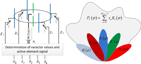
Figure 1 Illustration of BS-MIMO transmission using a 5-element ESPAR antenna

The ESPAR antenna should be able to adapt the Tx pattern per symbol period using one active and (M_T – 1) parasitic elements. BS-MIMO transmission is implemented, if the ESPAR antenna transmits the desired pattern $P\left(\phi ,n\right)$. This is achieved with proper readjustment of the variable reactance values (varactors) of the parasitic element loads ${\chi }_{i=\mathrm{1...}{M}_T-1}$. In order to determine the varactor values that produce the desired pattern, the following relationship is used [2]:

$$P\left(\phi ,n\right)=a{\left(\phi \right)}^{\text{T}}i=a{\left(\phi \right)}^{\text{T}}{v}_s\left(n\right){\left(Z+X\left(n\right)\right)}^{-1}{\left[\begin{array}{cccc}1& 0& \dots & 0\end{array}\right]}^{\text{T}}\text{ (5)}$$

where Z is the M_T × M_T matrix of the mutual coupling among the antenna elements, a(φ) the array manifold vector, i the vector of the currents that flow on the active and parasitic elements, v_s(n) the excitation signal of the active element and X(n) the diagonal matrix that contaibns the vararctor values $j{\chi }_{i=\mathrm{1...}{M}_T-1}$ of the parasitic elements during the n-th symbol. The specific algebraic representation assumes that the active element is placed in the first line of matrix X(n), thus [X]_1,1 = 50 Ohm since the active element is terminated to a 50 Ohm resistance. Calculation of desired load values can be performed by (5) with the use of a stohastic [7] or a genetic [10] algorithm. Assuming for simplicity that M_T=M_R=M, the reception is implemented with the sequential alternation of the basis patterns during a symbol period (with an M-times oversampling rate).

The basis patterns are selected to form an orthonormal set of functions for two main reasons. Firstly, in [2] a procedure that allows the use of the common MIMO input-output relationship (1) to also describe BS-MIMO transmission is presented. Assuming a channel with K discrete scatterers and H_g is the K × K complex, diagonal scattering matrix, then the beamspace transmission can be modelled as:

$$y_{bs}=H_{bs}{x}_{bs}+n_{bs}=B_R^H{H}_g{B}_T{x}_{bs}+n_{bs}\text{ (6)}$$

where the K × M matrices B_T/R contain the values of the M basis patterns in transmitter and receiver towards the direction of the scatterers (Angles of Departure in the Tx and Angles of Arival in the Rx). It is emphasized that in beamspace x_bs and y_bs are not directly related to the element currents but their relationship with the currents is provided by (5). Thus, H_bs and H have completely different structures due to the performed linear transformations [2]. Investigation of (6) leads to the conclusion that conventional MIMO algorithms can also be used for BS-MIMO systems with no significant changes. Secondly, it is proved that the (Tx or Rx) correlation matrix for each MISO cylindrically isotropic 2-D channel that describes the ideally rich scattering propagation environment is given by:

$$R_{hh}=\left(1/M^2\right)I_M\text{ (7)}$$

where I_M is the M-identity matrix. Thus, the selection of the orthonormal basis patterns leads to the best possible correlation properties for rich scattering environments. In [6], it was shown that the system maintains its strong correlation properties in realistic radio channels. Therefore, it is expected that matrix H_bs will provide aDoF that are statistically expected to approach M regardless of the interelement distance d and thus the system will provide better support for the transmission of multiple data streams.

The aDoF can be determined with the SVD of the channel matrix. Moreover, the result of the SVD can be used to develop and implement an adaptive pattern reconfiguration scheme to maximize capacity and channel efficiency. In [6], a pattern adaptation rule, similar with the conventional MIMO SVD-based precoding, is proposed. If H_bs = UΣV^H, then it is proved that the beamspace channel can be exploited optimally with the use of adapted basis patterns at Tx and Rx. More specifically, the new orthonormal bases are given by:

$${\overline{B}}_R=B_R{U}_{aDoF}, {\overline{B}}_{\text{T}}\text{=}{B}_{\text{T}}{V}_{\text{aDoF}}\text{ (8)}$$

The subscript of U and V defines that the first aDoF columns of the matrices are used, reducing the used basis patterns, if necessary, with respect to the supported aDoF. In order to practically implement and evaluate the pattern adaptation scheme, it is necessary to extract accurate channel estimates. Moreover optimization of the capacity can be performed with proper power allocation among the patterns with the use of the waterfilling algorithm. More specifically, the power per pattern is assigned with the following formula:

$$p_i={\left(\mu -\frac{{\sigma }_n^2}{{\sigma }_i^2}\right)}^{+}\text{ (9)}$$

where ${\sigma }_n^2$ is the noise variance, σ_i is the i-th singular value of Σ and μ is a constant that depends on the total available transmitted power i.e. $P_{tx}={\displaystyle \sum _{i=0}^{M-1}{\left(\mu -\frac{{\sigma }_n^2}{{\sigma }_i^2}\right)}^{+}}$. Superscipt + indicates that the expression is valid for positive values of the argument (otherwise p_i = 0). If $W=\text{diag}\left[\begin{array}{ccc}{p}_1& \dots & p_{aDoF}\end{array}\right]$ is the power allocation matrix, then the transmitted pattern towards the scatterers is given by:

$$p_T=B_T{V}_{\text{aDoF}}\sqrt{W}{x}_{bs}\text{ (10)}$$

This paper assumes that sets of 3-element or 5-element ESPAR antennas are used in Tx and Rx in order to evaluate BS-MIMO performance, while a 3-element or 5-element ULA with the same interelement distance d = λ/16 is assumed for the equivalent conventional MIMO system. The initial channel-unaware orthonormal basis patterns can be analytically extracted with the use of a proper othogonalization algorithm e.g. Gram-Schmidt. The analytical expressions for the 5-element ESPAR antenna can be found in [5] and for the 3-element ESPAR in [8].

3. Channel Estimation in BS-MIMO

The equivalence between the algebraic representations of BS-MIMO and conventional MIMO systems can be exploited in order to transfer algorithms from the conventional systems [11] to the beamspace domain. Moreover, the presented channel estimation algorithms can be used for wideband, frequency selective channels. The delay is introduced as the third dimension and therefore the channel is transformed in a 3-D matrix H_bs(k) with k=0,1..L, where L is the maximum expected excess delay. In beamspace systems, each element of the channel matrix represents the complex gain between beams, that are expressed in the angular domain through the basis patterns. Frequency selectivity in a beamspace transmission is caused by energy from previously transmitted patterns that spreads in time due to the different propagation paths and corresponding delays of the radio channel. The delayed arrival of signals at the receiver causes InterSymbol Interference (ISI). Wideband BS-MIMO analysis is a subject for future work, however the presented channel estimation algorithms can be applied to frequency selective channels. The specific channel estimation algorithms assume that a training sequence (known to the Rx) is used. The training sequence is carried by the initial channel-unaware basis patterns forming the training patterns. Given the fact that M²(L+1) parameters are estimated, the training sequence length N_T for each MISO channel should be greater than M(L+1) samples (MN_T ≥ M²(L + 2)).

The algorithms for conventional MIMO systems in [11] decompose the channel estimation procedure in MISO channels. Îd’his decomposition is valid when uncorrelated spatial reception is assumed. For small-sized antennas the assumption of uncorrelated reception is false for conventional MIMO as shown in (3), however it is 100 % accurate for BS-MIMO systems. Thus, the channel for each received beam ${\mathbf{\text{h}}}_{bs,i}^{\text{H}}$ (k) (each line of the channel matrix) can be extracted separately to form the estimate of H_bs(k). In order to mathematically define the estimators, the 3-D matrices are rearranged and the following reshaped vector of parameters is defined for the i-th MISO channel:

$$g_i=\left[h_{i,0}^{bs}\left(0\right)\mathrm{...}{h}_{i,0}^{bs}\left(L\right)\left|\mathrm{...}\right|h_{i,M-1}^{bs}\left(0\right)\mathrm{...}{h}_{i,M-1}^{bs}\left(L\right)\right]\text{ (11)}$$

The observation vector for each MISO channel used by the estimators is:

$$z_i={\left[\begin{array}{ccc}{y}_{bs,i}\left(L\right)& \mathrm{...}& y_{bs,i}\left(N_T-1\right)\end{array}\right]}^T\text{ (12)}$$

It is observed that the estimators ignore the L first incoming samples that are affected from preceding symbols not contained in the training sequence.

3.1. Linear Least Squares (LS)

In compliance with the shape of the vectors defined in (11) and (12), a $\left(\left(N_T-L\right)\times M\left(L+1\right)\right)$ matrix is defined that contains the training sequences carried by the M basis patterns:

$$\begin{array}{l}X=\left[\begin{array}{ccc}{X}_0& \mathrm{...}& X_{M-1}\end{array}\right],\\ X_i=\left[\begin{array}{ccc}{x}_{bs,i}\left(L\right)& \dots & x_{bs,i}\left(0\right)\\ x_{bs,i}\left(L+1\right)& & x_{bs,i}\left(1\right)\\ ⋮& & ⋮\\ x_{bs,i}\left(N_T-1\right)& \dots & x_{bs,i}\left(N_T-L-1\right)\end{array}\right]\text{ (13)}\end{array}$$

The LS estimate is then given by:

$${\widehat{g}}_{i,LS}={\left[X^{\text{H}}X\right]}^{-1}{X}^{\text{H}}{z}_i\text{ (14)}$$

The resulted MISO mean squared estimation error is given by:

$${\epsilon }_{\text{LS,MISO}}={\sigma }_n^2\text{Tr}\left[{\left(X^{\text{H}}X\right)}^{-1}\right]\text{ (15)}$$

where ${\sigma }_n^2$ is the noise variance. For zero-mean uncorrelated errors with equal variances (since noise is generally assumed equal for all MISO channels), the LS estimator is the best linear unbiased estimator.

3.2. Minimum Mean Square Error (MMSE)

The mean squared error of the estimation is minimized with the MMSE that uses a priori information:

$${\widehat{\mathbf{\text{g}}}}_{i,MMSE}=\frac{1}{{\sigma }_n^2}{\left[R_{hh}^{-1}+\frac{X^{\text{H}}X}{{\sigma }_n^2}\right]}^{-1}{X}^{\text{H}}{z}_i\text{ (16)}$$

A priori information is contained in the correlation matrix R_hh of vector g_i, i.e. the correlation matrix of the i-th wideband MISO channel. For L=0 (flat channel) and for rich scattering environments [13], the correlation matrix is approximated by (7) since uncorrelated beamspace transmission is achieved. In case of a wideband channel, each diagonal element is replaced by an (L+1) × (L + 1) submatrix which is the correlation matrix for each beam in the delay domain. Assuming channels with uncorrelated scattering, R_sub will contain in its diagonal an estimate of the channel power delay profile per beam. If this information is unavailable, various empirical rules can be applied:

$$R_{\text{sub}}=\underset{\text{Large} \text{Delay} \text{Spread}}{\underbrace{\left[\begin{array}{ccc}1/\left(L+1\right)& & 0\\ & \ddots & \\ 0& & 1/\left(L+1\right)\end{array}\right]}}\text{or}\underset{\text{Small} \text{Delay} \text{Spread}}{\underbrace{\left[\begin{array}{ccc}1& & 0\\ & 0& \\ 0& & \ddots \end{array}\right]}}\text{ (17)}$$

In these expressions the matrices are normalized to unit power. The first case assumes uniform power delay profile and it should be used for channels with large delay spread. The second case initially assumes flat fading. However, the second approach results in a non-invertible matrix. In order to use this approach, low-power noise should be added to the zero-valued elements of the matrix diagonal. Although MMSE performs well using the aforementioned empirical rules, in slow varying channels better results can be achieved when the previous channel estimate is used to approximate the correlation matrix of the current channel. Thus,

$${\widehat{R}}_{hh}={\widehat{\mathbf{\text{g}}}}_{i,\text{old}}{\widehat{\mathbf{\text{g}}}}_{i,\text{old}}^H\text{ (18)}$$

However, the specific approximation has been proven sensitive to phase noise and it requires very low mobility. Better and stable performance is achieved with the use of the previous channel estimate as an approximation of the power delay profile, assuming uncorrelated scattering. In this case, ${\widehat{R}}_{hh}$ can be written as:

$${\left[{\widehat{R}}_{hh}\right]}_{i,j}=\{\begin{array}{c}{\left|{\left[{\widehat{\mathbf{\text{g}}}}_{i,\text{old}}\right]}_i\right|}^2, \text{if} i=j\\ 0, \text{if} i\ne j\end{array}\text{ (19)}$$

The procedure can be initialized using an empirical rule from (17).

The theoretically calculated estimated error is given by:

$${\epsilon }_{\text{MISO}}^{\text{MMSE}}=\text{Tr}\left[{\left(R_{hh}^{-1}+\frac{X^{\text{H}}X}{{\sigma }_n^2}\right)}^{-1}\right]=\text{Tr}\underset{\text{flat,rich scattering}}{\underbrace{\left[{\left(M^2{I}_M+\frac{X^{\text{H}}X}{{\sigma }_n^2}\right)}^{-1}\right]}}\text{ (20)}$$

where the result for a rich flat normalized channel is also provided.

3.3. Optimal Training Patterns

The training patterns are formed by sequential N_T linear combinations of the basis patterns with a properly selected training sequence. Since both LS and MMSE estimators depend on the inverse of the product X^HX, it is proved with the use of Lagrange multipliers that for given power of the training sequence, the errors are minimized when [18]:

$$X^{\text{H}}X=\{\begin{array}{c}{\lambda }_{LS}{I}_{\left(L+1\right)M},\text{ for LS}\\ {\lambda }_{MMSE}{I}_{\left(L+1\right)M}-R_{hh}^{-1},\text{ for MMSE}\end{array}\text{ (21)}$$

where the constants λ_LS and λ_MMSE are selected to satisfy the power constraints of the training sequence. For a flat, rich-scattering channel, or a wideband channel with large delay spread, the matrix R_hh is a scaled identity matrix and thus the LS and MMSE estimators have a common minimum. In this case, since X is by definition a Toeplitz matrix, a training sequence that diagonalizes X^HX and minimizes the estimation error is the Frank-Zadoff-Chu (FZC) sequence [11]. The sequence is placed in the 1^st column or row of X depending on which dimension is greater. The following columns/rows are filled with circular rotation of the previous column/row by an element. Thus, the FZC sequence size is either N_T – L or M(L+1). Since the sequence size must exceed the number of estimated parameters, an FZC sequence of N_T – L length is assumed. The FZC sequence is not a sequence of modulated symbols (e.g. using the QAM modulation), however it is mapped to the initial channel-unaware basis patterns with the same method as the data streams, forming the optimal training patterns. It is noted that channel estimation should always be made with the use of the channel-unaware patterns. The use of channel adapted patterns during the estimation stage may lead to false detection of the available aDoF, since the radio channel continuously changes in time. The optimal training patterns are given by:

$$\begin{array}{c}{P}_{\text{train}}\left(\phi ,k\right)={\displaystyle \sum _{i = 0}^{M-1}{B}_i\left(\phi \right)f\left(k-\left(i+1\right)L\right)}, k=\mathrm{0...}{N}_T-1\\ \text{where: }f\left(k\right)=\{\begin{array}{c}{e}^{\frac{j\pi Q{k}^2}{N_T-L}},\text{if }{N}_T-L\text{ even}\\ e^{\frac{j\pi Qk\left(k+1\right)}{N_T-L}},\text{if }{N}_T-L\text{ odd}\end{array}\end{array}\text{ (22)}$$

where Q is a constant coprime to N_T – L.

If R_hh is not a scalable identity matrix, the FZC sequences are not optimal for the MMSE estimator. From [17], it can be proved that the optimal training sequences can be found by linear transformation of the FZC. If R_hh = QΛQ^H is the eigenvalue decomposition of the hermitian matrix R_hh and since Q is an orthogonal matrix, then:

$$Q^{\text{H}}{X}^{\text{H}}XQ=\lambda I_{(L+1)M}-{\Lambda }^{-1}\text{ (23)}$$

which is minimized when Q^HX^HXQ is a diagonal matrix and based on the previous analysis, when Q^HX^HXQ + Λ^{- 1} is a FZC sequence.

In Fig. 2 and Fig. 3, mean squared estimation error results for a 5-element and a 3-element ESPAR antenna BS-MIMO system respectively are presented. The interelement distance in both scenarios was d = λ/16 and the WINNER II channel model [14] was used after proper modifications in order to support beamspace transmission [13]. The WINNER radio channels were downsampled for narrowband transmission (flat fading channels). The estimators had to determine M²=25 or 9 complex gains of H_bs. Training was performed with FZC sequences. The term samples/parameter is used as a measure of the training sequence length. If x training samples per parameter are selected, then the training sequence length per MISO channel is given by N_T=Mx. Evaluation was performed with 10,000 flat 'B2' (bad urban micro-cell environment) channels vs. SNR for various N_T values. For the MMSE estimator, the correlation matrix was set according to $R_{hh}=\left(1/M^2\right)I_M$. The simulation results (lines) and the theoretic results (markers) from (15) and (20) were identical, which also means that 'B2' and ideally rich scattering channels behave similarly in beamspace, as far as the estimation procedure is concerned. MMSE and LS results are practically equal for high SNR, while for low SNR MMSE performs better. The SNR value, where MMSE overcomes the LS estimator depends on the length of the training sequence. The investigation of the two Figures shows that the error values for e.g. 4 training samples/parameter are lower in the 3-element ESPAR scenario. This happens because for each MISO channel, the error is calculated as the sum of M error terms from the M transmitted beams. Since for the 5-element ESPAR M is greater, the error also increases. Accurate estimation at low SNR requires long training sequences. For example 30 samples/parameter produce error approximately equal to ε = 0.02 @5dB SNR for 5-element ESPAR, while the same error value is achieved with 20 symbols/parameter for the 3-element ESPAR.

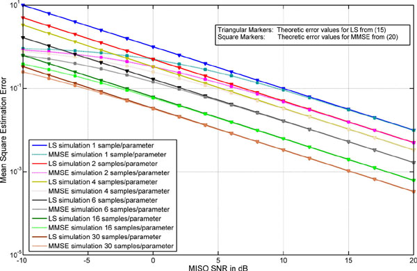
Figure 2 : Channel Estimation Error vs SNR in BS-MIMO for flat fading B2 WINNER channels and various training sequence lengths using a 5-element ESPAR antenna

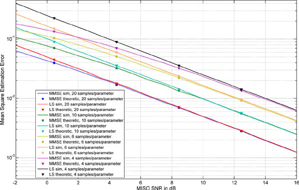
Figure 3 : Channel Estimation Error vs SNR in BS-MIMO for flat fading B2 WINNER channels and various training sequence lengths using a 3-element ESPAR antenna

The next step is to test the performance of the estimation algorithms in wideband beamspace channels. The previous 5-element antenna setup was considered. However, in this case the BS-MIMO system was assumed to occupy 1.5 MHz of bandwidth, and thus it cannot be considered narrowband. The training sequence length was 400 samples. Each signal frame contained 2,900 symbols (400 training samples + 2,500 data symbols) and the receiver was considered mobile (pedestrian user with velocity 3 m/sec). 2,000 'B2' WINNER channels were produced and the transmission of 30 frames of data was simulated. The WINNER channels were downsampled in the signal bandwidth (1.5 MHz). The maximum excess delay under these conditions was L + 1 = 5. Therefore, the algorithms should estimate M²(L + 1) = 125 parameters. In Fig. 4, the results of the evaluation are presented for various approximations of R_hh. It is seen that the MMSE algorithm despite the approximations, performs better than the LS. For the specific channels, the uniform power delay profile assumption (17) performs worse than the flat channel approximation (with addition of noise). The generic Cluster Delay Line (CDL) profile of the WINNER 'B2' channels [20] was also used in the diagonal of R_hh and the estimation algorithm performance was slightly improved. Finally the approximation of (19) was evaluated. During the first frame, the flat approximation was used and then for the 29 succeeding frames, the previous estimation was used. It is noted that the receiver is mobile, thus the channel response varies from frame to frame. The estimation error was further reduced. For comparison reasons, an ideal case is also presented in Fig. 4 where the MMSE operates with ${\widehat{R}}_{hh}=g_i{g}_i^{\text{H}}$, which means that the channel is actually known to the estimator.

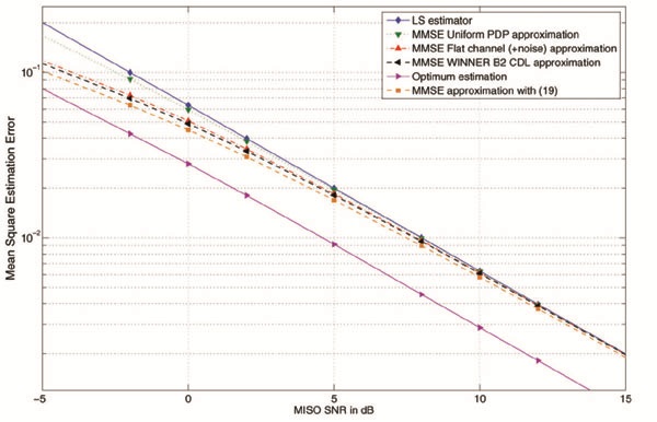
Figure 4 : Wideband Channel Estimation Error vs SNR in BS-MIMO for B2 WINNER channels (L=4) with training sequence length = 400 samples using a 5-element ESPAR antenna

3.4. Use of the Estimate for Pattern Reconfiguration

At the end of the estimation procedure, the channel matrix estimate ${\widehat{H}}_{bs}$ is available and it can be used for adaptive basis pattern reconfiguration according to the scheme proposed in [6]. The first step is to perform SVD decomposition ${\widehat{H}}_{bs}=\widehat{U}\widehat{\Sigma }{\widehat{V}}^{\text{H}}$. The overall estimation error is divided in the 3 matrices, however the errors of Ȗ and $\widehat{V}$ are more crucial since the deviations in Σ can be compensated with an one-tap equalizer at the receiver. These errors introduce interference between the transmitted parallel streams that can be called inter-beam or inter-pattern interference at both transmitter and receiver. Let's consider the virtual matrix representation ([2],[12]) of H_bs assuming an L-point uniform sampling $(L=2\pi /\Delta \phi )$ in the azimuth plane. The basis patterns at the virtual directions are given by the (L × M) matrices ${\tilde{B}}_{T/R}$. The virtual channel matrix [12] is defined by the following equation:

$$H_{bs}={\tilde{B}}_R^{\text{H}}{H}_b{\tilde{B}}_T\text{ (24)}$$

If ${\Xi }_u$, ${\Xi }_v$ are the estimation errors of $\widehat{U}$ and $\widehat{V}$ respectively then after pattern adaptation using the channel estimate, the channel matrix is given by:

$$\begin{array}{c}{\widehat{U}}^{\text{H}}{H}_{bs}\tilde{V}={\left(U+{\Xi }_u\right)}^{\text{H}}{\tilde{B}}_R^{\text{H}}{H}_b{\tilde{B}}_T\left(V+{\Xi }_v\right)=\Sigma +\\ +\left({\Xi }_u^{\text{H}}{\tilde{B}}_R^{\text{H}}\right)H_b{\tilde{B}}_{T}V+U{\tilde{B}}_R^{\text{H}}{H}_b\left({\tilde{B}}_T{\Xi }_v\right)+{\Xi }_u^{\text{H}}{H}_{bs}{\Xi }_v\end{array}\text{ (25)}$$

For high SNR, the last term with the product of the error matrices can be omitted as insignificant. The first error term expresses the inter-pattern interference due to the Rx adaptation while the second term due to Tx pattern adaptation. Therefore, the interfering patterns can be defined. The interfering patterns are the estimation error terms from the singular vector matrices expressed in the angular domain. If the adapted channel-aware basis patterns beamform the signal towards different angles, physical compensation of the interfering patterns is offered, since the interfering energy will be significantly reduced. This means that in channels with big and discrete scatterer clusters, the effects of the estimation error will be smaller due to the angle separation.

In Fig. 5a an example of the estimated reconfiguration patterns is presented compared with the ideal patterns that were calculated assuming perfect channel knowledge for a 'B2' channel of the 3-element ESPAR system. This channel has 2 aDoF and thus provides 2 channel-adapted orthogonal patterns. Estimation was performed with 13 dB mean MISO SNR. The SVD reallocates the power resources in favour of the first pattern in terms of SNR. Thus, the orthogonal path supported by the first pattern provides SNR = 16 dB while the second pattern provides SNR = 5 dB. Fig. 5a shows that the first pattern is estimated perfectly. This is also true when mean MISO SNR is reduced to 7 dB, where the path supported from the first pattern achieves SNR=12dB. However, the second pattern produces high error values in low SNR, which is not quite clear by the investigation of the absolute values of the patterns in Fig. 5a. Fig. 5c shows that the interfering pattern is actually more powerful than the basis pattern itself due to significant random phase shifts. This is caused as a mathematical reaction of the SVD in the presence of powerful noise. Nevertheless the total squared error of H_bs will remain relatively low because the term ${\Xi }_u^H{H}_{bs}{\Xi }_v$ of (25) has now significant power and opposes the error increase. In Fig. 5b, a typical case is presented where the second interfering pattern does not aim towards the same direction with the first pattern and therefore, the effect of the estimation error that occurs is practically zero.

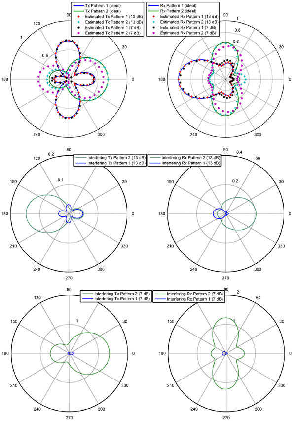
Figure 5 : Pattern adaptation for a typical WINNER B2 channel: a) Adapted patterns, ideal and via estimation (13, 7 dB SNR) b) Interfering patterns for the example (13 dB) c) Interfering patterns for the example (7 dB), [8]

The result in (25) can be used to calculate the SNR degradation due to the channel estimation error in a BS-MIMO system with adaptive pattern reconfiguration. More particularly, if E is the M × M matrix that contains the inter-beam interference terms, given by:

$$E=\left({\Xi }_u^H{\tilde{B}}_R^H\right)H_b{\tilde{B}}_{T}V+U{\tilde{B}}_R^H{H}_b\left({\tilde{B}}_T{\Xi }_v\right)+{\Xi }_u^H{H}_{bs}{\Xi }_v\text{ (26)}$$

then the total BS-MIMO inter-pattern interference can be calculated by:

$${\epsilon }_{\text{MIMO}}={\Vert E\Vert }_F^2-{\left(\text{Tr}\left[E\right]\right)}^2\text{ (27)}$$

and the inter-pattern interference caused at the i-th receiving beam (MISO interference) is given by:

$${\epsilon }_{MISO}^i={\displaystyle \sum _{k=1,k\ne i}^M{\left|{\left[E\right]}_{i,k}\right|}^2}\text{ (28)}$$

It is noted that the results in (27) and (28) do not include self-inflicted distortion that is expressed by the diagonal elements of E. This error, if detected, can be removed by the system equalizer.

4. Evaluation of BS-MIMO through Simulation

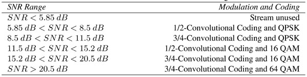
In order to evaluate the performance of a BS-MIMO system that includes pattern adaptation and realistic channel estimation algorithms through simulation, two equivalent pairs of systems were assumed: a conventional MIMO system with 3-element or a 5-element ULA vs. the BS-MIMO system with a 3-element or a 5-element ESPAR antenna. The inter-element distance was set to d = λ/16 for all systems. Moreover, both systems use SVD for precoding or pattern reconfiguration as well as a similar channel estimation techniques (45 and 100 training samples for 3-element and 5-element systems respectively) as described in [11] and Sec. 3. The systems use a simple coding rule that ensures BER < 10^-4 in order to achieve a certain level of adaptivity and exploit in a simple way the radio resources. Convolutional coding was applied using the default MATLAB Trellis structure poly2trellis (7,[171 133],171). The applied automatic modulation and coding rule is presented in Tab. 1. Each time an estimated singular value indicates a channel with SNR < 5.85 dB, the corresponding pattern is rejected and DoF/aDoF are reduced. It is noted that optimization of the adaptive coding and/or modulation rule was not an objective of this study.

Table 1 The Automatic Modulation and Coding rule.

A set of 3,000 flat 'B2' channels was applied to both systems. Moreover, in [19] it is stated that beamspace reception is performed in an M times oversampling rate, thereby noise power is increased by M at the BS-MIMO receiver.

Noise power was defined from the target mean BS-MIMO SNR. Every WINNER beamspace channel is normalized with its Forbenius norm: ${\overline{H}}_{bs}=H_{bs}/{\Vert H_{bs}\Vert }_F$. In order to compare equivalent systems, the respective conventional MIMO matrix (that is produced by the same clusters of scatterers [13]) is also normalized by the same factor multiplied by $\sqrt{\overline{M}}(\overline{H}=\sqrt{\overline{M}}H/{\Vert H_{bs}\Vert }_F$), where $\overline{M}$ are the identified aDoF of the beamspace system. This means that, since $\overline{M}$ patterns are transmitted when adaptive pattern reconfiguration is used, the oversampling rate at the BS-MIMO receiver will also be reduced from M to $\overline{M}$. Consequently, the relative noise increase compared to the conventional system will also be reduced.

The results of this section are provided vs. the mean SNR in the beamspace per MISO channel. If P is the available transmitted power, then the mean BS-MISO SNR is defined as:

$${\text{ SNR}}_{\text{bs,MISO}}=\frac{P}{M{\sigma }_n^2}\text{ (29)}$$

The SNR value of (29) is used as a reference and as the x-axis in the provided figures of the section. Based on the above analysis, the corresponding SNR for the conventional MIMO system is given by:

$${\text{ SNR}}_{\text{conv,MISO}}=\frac{\overline{M}\times {\text{SNR}}_{\text{bs,MISO}}{\Vert H\Vert }_F^2}{{\Vert H_{bs}\Vert }_F^2}\text{ (30)}$$

During this study, a method to bypass the drawback of the BS-MIMO noise level was identified through proper pulse shaping and filtering. However, since it is work-in-progress, the current evaluation includes the $\overline{M}$-times noise power increase in BS-MIMO.

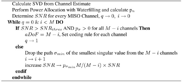
The instantaneous MISO SNR for each channel in SVD-based systems varies significantly from the value in (29) depending on: a) the singular value of the specific MISO channel and b) the power allocation rule (e.g. waterfilling) and the power adaptation that ensures that Tx power will remain equal to P when less than M DoF/aDoF are available. An iterative rule is used to determine the available channels and the corresponding SNR. If the SNR < SNR_thres for the channel that corresponds to the smallest singular value σ_min, the channel is rejected and the power for the rest of the channels is adjusted to: SNR $\to p_{{\sigma }_{min}}M/(M-i)\times SNR(i=1)$. Then, the smallest remaining singular value is checked and i → i + 1, until all values are greater than SNR_thres(=5.85 dB for these scenarios). The algorithm is described in Algorithm 1.

Algorithm 1: DoF/aDoF and assignment of coding rule

A noise power estimation stage is also incorporated in the receiver allowing the estimation of SNR degradation due to the channel estimation error. The results in terms of spectral efficiency are presented in Fig. 6 for the 5-element systems and in Fig. 7 for the 3-element systems. BS-MIMO outperforms the conventional system, especially in high SNR. It is also noted that regardless of the channel or the noise power the conventional system rarely exceeds the 2 DoF. Moreover, in many cases the 3-element conventional system degenerates to SISO. BS-MIMO on the other hand manages to achieve parallel transmission in the majority of the cases for high SNR. As noise power increases, BS-MIMO converges to the conventional MIMO behaviour maintaining a small advantage. At low SNR, both BS-MIMO and conventional MIMO turn into SISO and are set to operate with the same rules, therefore their performance is identical. Some steps or plateaus that can be seen in the figures are the result of the used adaptive modulation and coding rule. Another observation is that estimation appears to work less efficiently in the BS-MIMO case since the deviation of bits per symbol from the respective curve with perfect channel state information is higher. However, this is not accurate. It is reminded that noise is increased by M in the training period of the BS-MIMO system (regardless of the $\overline{M}$ aDoF, since estimation is performed for all M MISO channels) and therefore the difference in the performance of the estimator is due to the increased mean squared error caused by the inherent SNR degradation. In fact the performance of the estimator seems to be adequate despite of the increased by 7 dB noise level for the 5-element system and 4.77 dB for the 3-element system. Results for the 3-element BS-MIMO are also provided in [8]. Nevertheless, it must be noted that: a) in [8] only QPSK modulation is used, therefore the spectral efficiency remains low, while in Fig. 7, a powerful channel may use up to 64-QAM, b) in [8] no power allocation algorithm (waterfilling) is used and c) in [8] E_b/N_o is used as the x-axis which compared with the MISO SNR leads to a shift of values by 3dB for QPSK modulation.

Figure 6 : Performance comparison between 5 element BS-MIMO and conventional MIMO systems in terms of Spectral Efficiency (net bit rate in the Physical Layer per Hz). The actual net bit rate is given by the value on the y-axis × system bandwidth (Perfect channel knowledge and LS estimation)

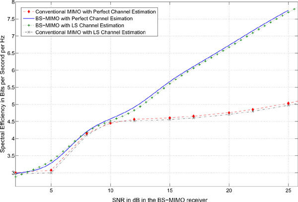
Figure 7 : Performance comparison between 3 element BS-MIMO and conventional MIMO systems in terms of Spectral Efficiency (net bit rate in the Physical Layer per Hz). The actual net bit rate is given by the value on the y-axis × system bandwidth (Perfect channel knowledge and LS estimation)

It is also clear that if the BS-MIMO system was not subjected to the increased noise level, the achieved bit rate would be even grater. In low SNR, where aDoF → 1, the noise level remains the same for both systems since no oversampling is required for the BS-MIMO receiver operation. However, in high and mainly in medium SNR ranges, lower noise would mean more aDoF, less coding redundancy and better estimation results. Noise reduction can be achieved with proper pulse shaping of the transmitted pulses and with the use of a filtered downsampling procedure in the receiver. This architecture will limit the noise increase factor to a small value (e.g. 1.5 depending on the filter transition bandwidth).

It is also noted that when perfect channel knowledge is assumed, the BER target (10^-4) was achieved for all cases. On the other hand, channel estimation error and the consequent SNR degradation resulted in slightly increased BER level, which means that in a limited number of cases the BER threshold for both BS and conventional MIMO system was exceeded. Finally given the fact that the used adaptive modulation and coding scheme is simple and not optimal, it is expected due to the existing theoretical capacity results [6] that the BS-MIMO bit rate advantage can become even grater.

5. Conclusions

This paper dealt with the subject of BS-MIMO channel estimation. Analysis of MMSE and LS estimators was performed through simulation. It was concluded that the estimation procedures are quite similar with conventional MIMO algorithms. The concept of interfering patterns was introduced and its physical meaning was presented. Finally, an attempt to evaluate BS-MIMO through link level simulation was made. BS-MIMO transceivers with adaptive pattern reconfiguration and practical, realistic reception algorithms that operate in WINNER 'B2' channels were assumed. It was confirmed that BS-MIMO systems outperform conventional MIMO for small interelement distances despite the increase of noise power due to oversampling. Prevention of the noise level increase is a subject for future work.

Acknowledgment

This paper is an extension of the work entitled “Channel Estimation and Link Level Evaluation of Adaptive Beamspace MIMO Systems” [8] that received the Best Paper Award in the Wireless VITAE conference of the Global Wireless Summit 2013. The research is co-financed by the European Union (European Social Fund-ESF) and Greek national funds through the Operational Program "Education and Lifelong Learning" of the National Strategic Reference Framework (NSRF) – Research funding Program: THALES Invensting in knowledge society through the European Social Fund, MIS379489.

References

[1] O. N. Alrabadi, J. Perruisseau-Carrier and A. Kalis. MIMO Transmission Using a Single RF Source: Theory and Antenna Design. In IEEE Transactions on Antennas and Propagation, vol.60, no.2, pp.654-664, 2012.

[2] A. Kalis, A. Kanatas and C. Papadias. A Novel Approach to MIMO Transmission Using a Single RF Front End. In IEEE Journal on Selected Areas in Communications, vol. 26, no 6, pp.972-980, August 2008.

[3] M. Wennstrom and T. Svantesson. An antenna solution for MIMO channels: the switched parasitic antenna. In 12th IEEE International Symposium on Personal, Indoor and Mobile Radio Communications, pp.159-163, vol.1, 2001.

[4] T. Ohira and K. Gyoda. Electronically steerable passive array radiator antennas for low-cost analog adaptive beamforming. In Proceedings of IEEE International Conference on Phased Array Systems and Technology, pp.101-104, 2000.

[5] V. Barousis and A. G. Kanatas. Aerial degrees of freedom of parasitic arrays for single RF front-end MIMO transceivers. In Progress In Electromagnetics Research B, vol. 35, pp.287-306, 2011.

[6] P. N. Vasileiou, K. Maliatsos, E. D. Thomatos and A. G. Kanatas. Reconfigurable Orthonormal Basis Patterns Using ESPAR Antennas. In IEEE Antennas and Wireless Propagation Letters, vol.12, pp.448-451, 2013.

[7] V. Barousis, A. G. Kanatas, A. Kalis and C. Papadias. A Stochastic Beamforming Algorithm for ESPAR Antennas. In IEEE Antennas and Wireless Propagation Letters, vol.7, pp.745-748, 2008.

[8] K. Maliatsos, P. N. Vasileiou and A. G. Kanatas. Channel Estimation and Link Level Evaluation of Adaptive Beamspace MIMO Systems. In Proceedings of Wireless VITAE, Global Wireless Summit, 2013.

[9] A. Paulraj, R. Nabar and D. Gore. Introduction to Space-Time Wireless Communications. Cambridge University Press NY-USA, 2008.

[10] E. Thomatos, P. Vasileiou, and A. Kanatas. ESPAR loads calculation for achieving desired radiated patterns with a genetic algorithm. The 7th European Conference on Antennas and Propagation, EuCAP, 2013.

[11] O. Weikert and U. Zolzer. Efficient MIMO Channel Estimation With Optimal Training Sequences. In in Proceedings of 1st Workshop on Commercial MIMO-Components and Systems (CMCS 2007), 2007.

[12] A. M. Sayeed. Reconfigurable Orthonormal Basis Patterns Using ESPAR Antennas. In IEEE Transactions on Signal Processing, vol.50, no.10, pp.2563-2579, 2002.

[13] K. Maliatsos, A. G. Kanatas. Modifications of the IST WINNER channel model for beamspace processing and parasitic arrays. In Proceedings of the 7th European Conference on Antennas and Propagation, EUCAP 2013, 2013.

[14] L. Hentila, P. Kyosti, M. Kaske, M. Narandzic and M. Alatossava. MATLAB implementation of the WINNER Phase II Channel Model ver1.1. In https://www.ist-winner.org/phase_2_model.htm, 2007.

[15] T. Ohira and K. Iigusa. Electronically steerable parasitic array radiator antenna. In Electronics and Communications in Japan (Part II: Electronics), pp.25-45, Wiley Subscription Services, 2004.

[16] V. I. Barousis, A. G. Kanatas and A. Kalis. Beamspace-Domain Analysis of Single-RF Front-End MIMO Systems. In IEEE Transactions on Vehicular Technology, vol.60, no.3, pp.1195-1199, 2011.

[17] J. Pang, J. Li, L. Zhao and Z. Lu. Optimal Training Sequences for MIMO Channel Estimation with Spatial Correlation. In Proceedings of the 66th IEEE Vehicular Technology Conference, VTC-2007 Fall, pp.651-655, 2007.

[18] X. Ma and L. Yang and G. B. Giannakis. Optimal training for MIMO frequency-selective fading channels. In IEEE Transactions on Wireless Communications, pp.453-466, 2005.

[19] R. Bains and R. R. Muller. Using Parasitic Elements for Implementing the Rotating Antenna for MIMO Receivers. In IEEE Transactions on Wireless Communications, vol.7, no.11, pp.4522-4533, 2008.

[20] P. Kyosti, J. Meinila, L. HentilaBains, et all. IST-4-027756 WINNER II D1.1.2 v.1.1: WINNER II channel models, 2007

Biographies

Konstantinos Maliatsos received his Diploma in Electrical and Computer Engineering from the National Technical University of Athens, Greece (NTUA) in 2003. He joined the NTUA Mobile Radio-Communications Laboratory (MRCL) working as an assistant researcher in various industry and research oriented projects. In 2005 he earned his Master’s degree in Business Administration from the postgraduate studies program “Techno-Economic Systems” organized by NTUA, National Kapodistrian University of Athens and University of Piraeus (UniPi), while he started working on his PhD entitled “Transmission techniques, Design and Analysis of Software Defined Radio – Cognitive Radio Adaptive wireless transceivers”. He received his PhD degree in 2011. As an assistant researcher he worked for 3 years on projects for the Greek General Secretariat for Research and Technology on Cognitive Radios and also participated in MRCL European projects. Currently he is working on his post-doctoral research on advanced MIMO techniques in the Department of Digital Systems of UniPi. He also continuous to cooperate with MRCL as a researcher for FP7 European projects. He has published more than 25 papers in International Journals and Conference proceedings. His research interests include Software Radio, Cognitive Radio and Dynamic Spectrum Access, Multicarrier Modulations, MIMO systems (conventional, beamspace, massive and distributed), Filter Bank theory, Synchronization for broadband wireless, Channel Modeling, Detection and Estimation theory.

Panagiotis N. Vasileiou received his M.Sc. Degree in 2012 in digital communications and networks with honors and the B.Sc. Degree in 2010, from the Department of Digital Systems in the University of Piraeus. He has been awarded with scholarships for the first place in the academic records in three several periods during the B.Sc. program and one scholarship during the M.Sc. Since November 2013, he is a Phd student at the Telecommunication System Laboratory, Department of Digital Systems, University of Piraeus, where he involved in various research projects with published work in various communities.

Athanasios G. Kanatas received the Diploma in Electrical Engineering from the National Technical University of Athens (NTUA), Greece, in 1991, the M.Sc. degree in Satellite Communication Engineering from the University of Surrey, Surrey, UK in 1992, and the Ph.D. degree in Mobile Satellite Communications from NTUA, in February 1997. From 1993 to 1994 he was with National Documentation Center of National Research Institute. In 1995 he joined SPACETEC Ltd. In 1996 he joined the Mobile Radio-Communications Laboratory as a research associate. From 1999 to 2002 he was with the Institute of Communication & Computer Systems. In 2000 he became a member of the Board of Directors of OTESAT S.A. In 2002 he joined the University of Piraeus where he is a Professor in the Department of Digital Systems. From 2008 to 2009 he has served as Member of the Senate of University of Piraeus. From 2007 to 2009 he served as Greek Delegate to the Mirror Group of the Integral Satcom Initiative. His current research interests include the development of new digital techniques for wireless and satellite communications systems, channel characterization, simulation, and modeling for future mobile, mobile satellite and wireless communication systems, antenna selection and RF preprocessing techniques, new transmission schemes for MIMO systems, and energy efficient techniques for Wireless Sensor Networks. He has published more than 120 papers in international Journals and conference proceedings. He has been a Senior Member of IEEE since 2002. From 1999 to 2009 he chaired the IEEE ComSoc Chapter of the Greek Section. This year he elected Dean of the School of Information & Communication Technologies of the University of Piraeus.