Enabling Wireless Sensor Nodes for Self-Contained Jamming Detection

Received 1 March 2014; Accepted 15 April 2014; Publication 2 July 2014

Journal of Cyber Security, Vol. 3 No. 2, 133–158.
doi: 10.13052/jcsm2245-1439.322
Copyright © 2014 River Publishers. All rights reserved.

Stephan Kornemann¹, Steffen Ortmann¹, Peter Langendörfer¹ and Alexandros Fragkiadakis²

¹ IHP, Im Technologiepark 25, D-15236 Frankfurt (Oder), Germany
² Institute of Computer Science, Foundation for Research and Technology-Hellas(FORTH), Heraklion, Crete

Abstract

Jamming is an easy to execute attack to which wireless sensor networks are extremely vulnerable. If the application requires reliability, jamming needs to be detected and reported in order to cope with this attack. In this article, we investigate different approaches to identify jamming. Available jamming detection schemes primarily suffer from the usage of fixed thresholds as well as required effort. We adapted a variance-based estimate of signal-to-noise ratio measurements, called significance analysis, to the minor resources and computing efforts of wireless sensor nodes. As a start, we used real measurement data for theoretical analysis of the methods under investigation. Independently of the location of the jamming device, our significance analysis approach provides an immediate indication of jamming and can in theory be run with almost least effort, i.e., with O(14). On top of that, we implemented this approach on our state of the art sensor node and tested it in a real world outdoor setting. Our jamming detection engine monitors the wireless channel with a sampling rate of 10 ms. It returns a jamming detection decision within less than 5 ms while though achieving a detection accuracy in between 84 to 99 percent.

Keywords

Jamming detection
Wireless sensor networks
Security

1 Introduction

Wireless sensor networks (WSNs) are more and more considered as a basis for new applications e.g. in the area of automation control or critical infrastructure protection. Such applications require a significant level of reliability. Jamming is an attack which needs to be considered as extremely dangerous. It can be easily executed by anybody since it does not need any detailed knowledge about the system to be attacked [10] nor expensive equipment. In addition its effect is significant since it immediately distorts the expected system behaviour.

Many projects [2–5, 11, 15–16] have proven fixed thresholds to be unsuitable for jamming detection in wireless networks no matter which channel characteristic is monitored. Beside physical conditions around the node, the distance to the jammer predominantly influences the changes in channel characteristics by jamming, e.g. the signal strength of the jammer obviously decreases with the distance to network under attack but still remains noticeable. Such behaviour can also be seen in Figures 2(a) and 2(b) in the next chapter. Since the location of a jammer is hardly to predict [7], sensor nodes cannot be pre-configured for reliable jamming detection, even if the jamming characteristic is known. Instead, sensor nodes must learn distinguishing regular from irregular (jamming) channel conditions. This is a difficult task since normal operation within the WSN, e.g., during contention phases, can look like jamming and by that cause false positives.

The contributions of this papers are:

Introduction of different mathematical approaches which are suitable to detect jamming without prior knowledge on thresholds, i.e., self adaptive approaches.
Analysis of the computational complexity of these approaches in order to evaluate whether or not they can be used on resource constraint wireless sensor nodes.
Theoretical evaluation of a suitable metric, called significance analysis, using real measurement data.
Realization and validation of significance analysis for real-time detection of jamming on wireless sensor nodes in practice.
Discussion of approaches to reduce the number of false positives and false negatives.

In the next section we overview existing approaches and assess application of those in WSNs. Section 3 analyses and compares computational and memory effort of feasible solutions. Based on that, we introduce our low effort approach for online jamming indication. Section 4 evaluates simulation results based of data taken from real measurements in the laboratory. Based on that, we present implementation detail as well as achieved detection rates of our significance analysis on state of the art sensor nodes. Finally, we discuss trouble-shooting issues and provide concluding remarks.

2 Related Work

Applying wireless communication, WSNs by nature are vulnerable to disturbances or even blockages of the wireless channel. Such interference may of course occur due to changes in environmental physics, such as objects moving or changing weather conditions, especially humidity and rain [1]. However, interference on wireless channels can also be willingly provoked by an attacker. Such behaviour is usually called jamming. Many different jamming models as well as respective counter measures have been researched in depth in the past. Among others, random, reactive [16], periodic [4, 8] or constant [14] jamming models are applied for both single and multi-channel [9] attacks. Analysis of existing models in unison have agreed reactive, either random or periodic, jamming models to be the most effective ones for WSNs due to their jamming performance and energy efficiency.

Almost the same number of different counter measures using different basic metrics have been proposed. In the following we overview and assess the usage of these metrics. Xu et al. [16] evaluated the usage of different packet-based metrics. The Packet Send Ratio (PSR) basically indicates the number of packets sent during certain time period. This is equivalent to the analysis of time needed to access the wireless channel, usually given as Carrier Sensing Time (CST) when using CSMA MAC protocols. Thereby, a node detects a possible jamming attack if it can only access the channel with packet rates below certain threshold. This approach certainly performs poor if jamming and channel characteristics are unknown and hence, suitable thresholds cannot be fixed. Xu et al. [16] and Cakiroglu et al. [3] further have tested the packet-based metrics Packet Delivery Ratio (PDR) and Bad Packet Ratio (BPR). PDR counts the number of packets successfully sent or the number of acknowledgements received respectively. Jamming may then be detected if the ratio of successfully transmitted packets in percentage falls below certain threshold. Despite suitable processing effort this metrics implies usage of acknowledgement-based communication, which causes significant effort especially in case of good channel conditions. By that it cannot be expected suitable for resource constraint devices like WSNs. Similarly to the PDR-based method, the BPR-based approach calculates the percental ratio between correct (good) and erroneous (bad) packets received. Obviously, this method can be used at the receiver side only. However, these approaches cannot reflect usage of WSNs in heavily interfered environments where packet losses result from ordinary operation. Both approaches further suffer from the usage of predefined thresholds. Similar problems and a substantial effort prevent from using Bit Error Rate (BER) as metric as proposed by Strasser et al. [12].

The metric best reflecting the physical conditions of the wireless channel is based on the Received Signal Strength (RSS). Using RSS the ratio between received signal power and received noise level, usually called Signal-to-Noise-Ratio (SNR), can be determined. From our point of view, SNR is the most suitable metric for jamming detection since any interference, whether or not caused by jamming, is reflected by changes of SNR. The challenge of analysing SNR for jamming detection is distinguishing abnormal (or anomalous) SNR from usual behaviour by assessing the actual SNR value. Jamming detection techniques based on SNR for wireless networks have been proven functional in several projects. Cabrera et. al. [2] determined a threshold-based jamming detection scheme for application in MANETs, called anomaly index. This approach probabilistically rates SNR drops at single nodes in a distributed decision process at respective cluster heads but still requires to set jamming thresholds at the cluster head. To get rid of the necessity to configure fixed thresholds, which is infeasible due to the unknown location of the jammer and unforeseeable channel characteristics, the network must “learn” usual SNR by itself. The most common SNR-based approaches exploit the standard deviation [11] or the variance of SNR readings [4, 13] to rate the occurrence of interference based on previous trend of SNR. Despite partially outstanding detection performance, these approaches cannot be used in sensor networks due to effort required, as we will show in the next section. We will also introduce our significance analysis approach that circumvents presented disadvantages when using variance of SNR as metric for jamming detection.

3 Math & Computational Effort

To determine jamming by changing SNR requires to contrast actual SNR values with expected ones. We indicate the significance of changes in the SNR as the degree of deviation from the expected range of values learnt from previous trend. This expected range of values is determined by the average of previous values to a lesser or greater degree of the variance of those. Determining the average and the variance of previous readings is not very complex according to mathematics, but it originally is unsuitable for sensor networks due to the calculation and memory effort. This especially holds true when it is used for jamming detection, where every new SNR value has to be processed immediately. Hence, the effort for processing one single SNR value is to be determined. In the following, we introduce the math and respective effort in detail and point out the main drawbacks. We finally show how to adapt these calculations to the needs of limited devices like sensor nodes.

3.1 Standard Variance

The variance indicates the range of values where the next reading is most likely in. We propose to apply a maximum likelihood estimate to determine the variance of previous readings σ_m, see Equation 1. The variance originally requires to use all previous (here n) readings for calculating the average value x and the differences of x to all n previous readings x_i. In summary, processing a new reading requires 2n additions, n subtractions and squares, plus one division and one root extraction operation. Hence, the calculation effort of a single run is O(4n + 2), which finally equals to O(n). In addition, the standard variance requires a large amount of memory due to the necessity to store all previous n values. Even though we do not consider the additional overhead required for memory access, the standard variance is unsuitable for sensor networks due to both calculation and memory efforts. Since we intend using the variance of the SNR for online jamming detection, both parameters need to be significantly reduced to be applicable for sensor networks. Hence, we adapted the standard calculation to sensor needs by applying the parallel axis theorem and a customised sliding window derivative.

$σ_{m =} \sqrt{\sum_{i = 1}^{n} {(x_{i} - \bar{x})}^{2};} \bar{x} = \frac{1}{n} \sum_{i = 1}^{n} (x_{i}) (1)$

3.2 Reducing Calculation and Memory Effort

Obviously, on the fly processing of SNR readings must be very fast and may not depend on the number of values (n) used. The parallel axis theorem substitutes x by the average formula given in Equation 1. It allows processing consecutive sensor readings without the need to have all previous values available. Instead, only the sum of measurements and the sum of measurements squares need to be refreshed and stored, see Equation 2.

$\begin{array}{l} σ_{m} = \sqrt{(\frac{1}{n} \sum_{i = 1}^{n} x_{i}^{2}) - {\bar{x}}^{2}} = \sqrt{(\frac{1}{n} \sum_{i = 1}^{n} x_{i}^{2}) - (\frac{1}{n} \sum_{i = 1}^{n} x_{i})^{2}} \end{array} (2)$

Applying the parallel axis theorem fixes the calculation effort to eight operations O(8) per processing. It only requires to 2 additions, 2 divisions and 2 squares plus one subtraction and one root extraction. Even the memory effort is very low. It requires to store three numbers only, i.e., the sum of measurements, the sum of measurements squares and the entire number of processed readings. Unfortunately, these sums are the main drawback of this approach. The SNR usually varies below 100 dB and hence, the squares of SNR readings may be very huge. Further the number of processed SNRs can rapidly increase and result in huge sums used for calculating the variance with the parallel axis theorem. The microcontroller used on sensor nodes usually apply a 16 bit or a 20 bit architecture. Due to its energy efficiency we use the 16 bit MSP430 microcontroller from Texas Instruments on our nodes. Consequently, the 16 bit architecture limits the size of the sums to 65536.

3.3 Adaptation to Sensor Node Needs

To keep the sums adequately low, we propose to include only a certain number of previous readings specified by an adaptable sliding window s in the calculation. The sliding window approach provides two benefits. It allows to influence the size of the sums as well as to properly adapt the number of considered measurements to the application. For example, SNRs of past days may be not of interest for jamming detection, whereas the readings of the last ten minutes may be much more important for comparison and evaluation. Note, we also have considered reducing the SNR value by a factor before processing, e.g., dividing SNR values by 10 or 100. By that, we may unnecessarily introduce processing overhead since we cannot guarantee the availability of hardware-accelerated floating point arithmetic.

Obviously, the sliding window approach falls back into O(s) computational effort and requires to store s numbers in memory. Applying the parallel axis theorem allows to get rid of stored measurements as already shown, but is in principle unsuitable for the sliding window method, which requires these measurements. To allow efficient processing on sensor nodes, we propose combining both methods in σ_s by estimating the measurements within the sliding window. The important values of the parallel axis theorem are the sum of measurements and the sum of measurement squares, as mentioned. Originally, these sums are updated at every sensing interval by processing on the next sensor reading. To apply the sliding window method, the current measurement is added to the sums whereas the expected values are subtracted. The expected values are given by the average of the previous window, see Equation 3. For estimating the sum of measurements and the sum of measurement squares within the window, our approach additionally introduces only two division, two addition and two subtraction operations per single processing. In comparison to the original parallel axis theorem, the calculation effort of our approach is O (14). It also gets by with storing 3 numbers only, which are both sums and the size of the sliding window. Table 1 presents the efforts of discussed approaches in at nutshell.

$σ_{s} = \sqrt{\frac{1}{s} (\sum_{i = n - s - 1}^{n - 1} x_{i}^{2} + x_{n}^{2} - {\bar{x}}^{2}) - {(\frac{1}{s} (\sum_{i = n - s - 1}^{n - 1} x_{i} + x_{n} - \bar{x}))}^{2}} (3)$

Table 1 Comparison of computational and memory effort of approaches introduced. Despite of best effort, rapidly growing sums prevent from using the parallel axis theorem on 16 or 20 bit architectures

Method	Calculation	Memory
Variance	O(4n+2) = O(n)	n numbers
Parallel Axis Theorem	O(8)	2 numbers
Significance indicator	O(14)	3 numbers

3.4 How to Apply Estimated Significance of Changes

The variance of previous SNR readings (within the sliding window) provides the basis to give a statement about actual SNR readings. It enables to decide whether actual readings meet expected parameters or not. It further allows to assess how far new readings deviate from the expected scope. Therefore the system determines the significance indicator, which states by what multiple the actual reading diverges from the variance. Due to the parameters learnt from the variance of the measurements within the sliding window, the indicator automatically detects significant deviations without the need for predefined thresholds. That way, we expect enabling sensors to apply equal SNR processing for location-independent jamming detection.

4 Assessment of the Significance Analysis Approach

To give a proof of concept, we applied our approach on large data sets taken from our colleagues work presented in [4]. They set up a wireless network topology collecting Signal-to-Noise Ratio (SNR) measurements at different devices. Please note, their work originally focuses on general wireless networks instead of wireless sensor nodes. Used nodes were equipped with Mini ITX boards, with 512 MB RAM and a 80 GB hard disk. They are also equipped with Atheros NMP 8602 802.11 a/b/g wireless cards, controlled by the Madwifi MAC driver (version 0.9.4), on Ubuntu Linux.

4.1 Experimental Setup

Figure 1 represents the network topology used. The sender sent UDP traffic to the receiver at a constant rate of 18 Mbps. All measurements collected at the sender, the receiver and a monitor have been recorded for later processing. Sender, receiver and monitor all operate on channel 56. The network interface of the monitor was set to monitor mode, hence received all packets sent on this channel. Jamming is performed by using two further nodes, i.e., the evil sender and the evil receiver. These two nodes operated on channel 52, which is adjacent to channel 56 and hence, produces interference. The solid lines in Figure 1 represent a dedicated wired backbone for running the experiments. The evil sender periodically transmitted data with different inactive phases at a transmission power and rate of 13 dBm and 6 Mbps, respectively.

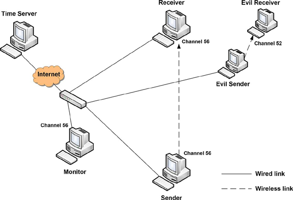
Figure 1 Network layout taken from [4]

4.2 Evaluation Results

Figure 2(a) shows the impact of the evil communication on the SNR at the (not-jamming) sender and Figure 2(b) at the (not-jamming) receiver respectively. These figures also show short influences, from second 44.0 to 45.5 and long influences, from second 46.2 to 47.2. These result from the normal protocol behaviour between evil sender and evil receiver. Due to this behaviour jamming detection in wireless networks is challenging. Based on their measurements our colleagues successfully tested their intrusion, or jamming, detection algorithms. For further details please refer to their work in [4]. However, even though their approach provides good detection results, necessary calculation and memory effort of the algorithms used are far from being useable for WSN. Therefore, we tested our approach based on significance indication, which requires significantly lower effort, on the same data sets of SNR measurements. Figures 3(a) and 3(b) clearly show that our significance indication reliably detects all deviations in the SNR value. In addition, it reacts faster than the variance method, see the more detailed Figures 4(a) to 4(d) showing a short jamming period. This holds true on each falling edge of the SNR values independently of the position of the jamming device. From our point of view the detection speed is of high importance since it can give the network under attack time to initiate proper counter measures. We are aware of the fact that there is not much a sensor node can do under jamming. But, storing sensed data, changing the wireless channel, trigger an alarm that jamming is ongoing are potential counter measures, and help to provide data for forensics and may be even a basis for a network manager to start counter measures, such as go and search the jamming device. On the one hand the high sensitivity of our significance approach is positive since it allows for detecting jamming from various positions within the WSN avoiding to set thresholds, which depend on the location of the jamming device. On the other hand triggering a jamming alarm whenever contention leads to a variation in the SNR value is unwanted since it leads to a significant number of false positives. In order to avoid false positives we are analysing the duration of the changes of the significance value. If it drops down to its initial value within the next values the change is not interpreted as jamming, since a jamming attack is considered to last longer. Our experiments figured out that drops in significance values lasting longer than ten percent of applied window size most probably identified a jamming period. Figures 4(a) to 4(d) display very short time slot with single or short drops in SNR with the associated variance and significance indication values. These figures clearly show that the duration of the significance value can be used as an indicator for jamming, due to its sensitivity. In case of jamming, i.e. second 45.16 from sender (Figure 4(a)), the significance indicator value stays high, whereas it drops down quickly in case of accidental increase of the SNR value. In contrast to this the variance method does not really allow to differentiate between accidental changes in the SNR value and intentional changes, i.e., jamming attacks. This is due to the fact that the variance analysis values do not change back quickly enough. Figures 4(a) to 4(d) clearly show that they stay high even after a quick recovery of the SNR value.

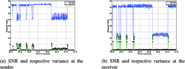
Figure 2 Influence of jamming to Signal-to-Noise Ratio (SNR) at sender and receiver. It clearly shows the impact of jamming on SNR to vary according to the distance of the jammer. The SNR readings at the receiver, which is located in close distance to the jammer, consider-ably show larger drops than those at the sender. These drops consequently also lead to local amplitudes in the variance

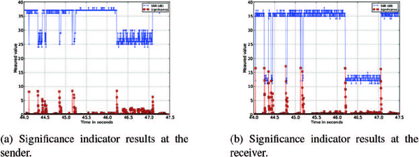
Figure 3 Measured Signal-to-Noise Ratio (SNR) and results of the low-cost significance indicator approach based on SNR readings at sender and receiver

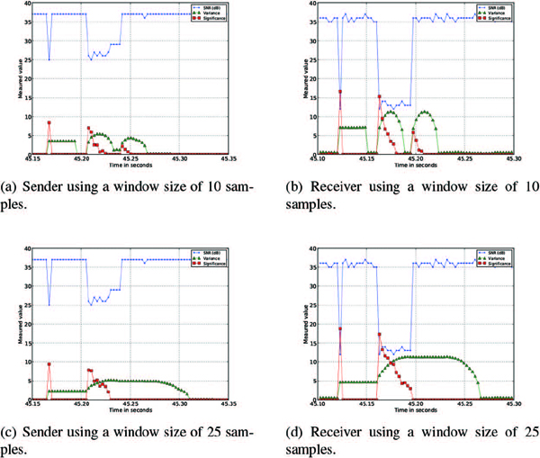
Figure 4 SNR, variance and significance indicator during single SNR drop and a short jamming period. Whereas the variance lags behind SNR changes, the significance indicator directly responds to each change

A high significance indicator reflects the difference between the expected SNR value and the actually measured one. In other words, the significance indicator value is zero as soon as the measured value is close to the expected one. Since the expected SNR value changes slowly over time, i.e., it increases only gradually from measurement to measurement, the size of the sliding window influences the sensitivity of the significance indicator approach. In contrast to the immediate reaction of the significance indicator approach, the variance analysis only indicates changes in the expected SNR value. By that the indicated deviation between two measurements is much smaller. In addition with continuous change in SNR values, the expected SNR and the variance converge to the actual SNR value. When the variance has reached its local maximum, the change of the SNR is fully reflected by the values of sliding window determining the variance. Thereafter only new changes may be registered and the variance value moves slowly back.

4.3 Handling False Positives & False Negatives

The size of the sliding window examined to determine whether or not the jamming indication value drops back or not, has a significant impact on the speed with that the indication value drops down. For a window size of 10 samples the values of both approaches drop down to the initial value, but with different speed. The significance indicator drops down almost immediately whereas the variance analysis needs several milliseconds. If the window size is prolonged to 25 values, see Figures 4(c) and 4(d), both approaches react slower in case that the SNR value has changed for longer than single or few measurements. For improving the correctness of the significance indicator approach this behaviour is beneficial, since the value stays high longer than with shorter windows, i.e., it can be taken more seriously. For extremely short variations in the SNR value the significance indicator value still reacts immediately, in other words, there we do not loose accuracy.

There is another not yet reflected aspect when deciding whether changes in the SNR shall be interpreted as jamming or not. The type of MAC protocol is an important factor. In normal contention based MAC protocols our considerations are valid, but are they still true when the MAC protocol applies a certain type of schedule? In such environments even very short periods of interference (dips in the SNR) might be due to jamming. What we mean is that a sophisticated jammer could try to block a selected time slot, i.e., to interrupt the connection of a single device. As additional means to detect such situations, we propose to specify the type of MAC and to record in which MAC time slot variances of the SNR are recorded. If it becomes apparent that a specific time slot is more often affected than others, jamming might be the correct interpretation independently of the adaptation speed of the significance indicator value.

5 Significance Analysis Based Jamming Detection

To give a real proof of evidence of our approach, we certainly needed to implement the presented mathematical approach on a state of the art sensor node rather than using data measured in a laboratory network set-up only. Therefore all details and experimental results provided in this section result from implementing the significance analysis on our own sensor node platform presented in the next subsection.

5.1 Applied Sensor Node Platform

Our own sensor node platform used for implementing the jamming detection approach was originally developed for monitoring vital and environmental of fire-fighters in action (Piotrowski et al.2010). In this platform we have three different radio transceivers in parallel, these are:

TI CC1101: Low cost transceivers working in the 868 MHz band
TI CC2500: Low cost transceivers working in the 2.4 GHz band
TI CC2520: ZigBee TM Transceiver working in 2.4 GHz band

We applied two pin and logic compatible transceiver chips working in different radio frequency bands, i.e. the first in the European 868 MHz band and the second in the 2.4 GHz. The third transceiver (ZigBee) is also working in the 2.4 GHz band and provides 802.15.4 support. It was applied to be able to communicate with other known node platforms. The sensor node is empowered by the MSP430F5438 Microcontroller from TI. The complete sensor node is depicted in Figure 5. Due to it’s redundancy in radio connectivity, our platform provides the ideal basis to implement and test different jamming scenarios with one setting of nodes. All results presented in this section have been measured on this platform.

Figure 5 Top view of the applied sensor node platform in comparison to the size of a 1 Euro coin

5.2 Concept of Jamming Detection

The concept presented here is based on several components, which are depicted in Figure 6. RSSI values from the radio module (RF module) are used as input data. The first component of the jamming detection is a significance analysis based on the mathematical approaches presented in the previous section 3.3. The result of this component are the significance changes in the RSSI values. We assume a large change in significance value to be caused by an active jammer. This information is used to generate an event to be evaluated by a following peak detection algorithm. In most peak detection algorithms a fixed threshold is used, but is not acceptable in this context. To decide between week and strong deflection, we use a dynamic threshold which is calculated with the Heaviside function given in equation 4.

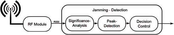
Figure 6 Concept of jamming detection

$Θ {(x)}_{p e a k} = (\frac{1}{s} \sum_{i = n - s - 1}^{n - 1} x_{i} + x_{n} - \bar{x}) - (\frac{\max (x_{n}, x_{n - 1}, ...., x_{n - s - 1})}{2}), x \in ℕ (4)$

The last component of the jamming detection engine is the decision control, which finally signals whether jamming is ongoing or not. The flowchart of the engine is shown in Figure 7. First the engine checks whether an event was generated by the peak detection. If that is true then the old (avg_old) is compared to the new (avg_new) average value of the RSSI input data. This branch corresponds to the formula 5. The second branch is used to solve two problems. The first challenge is that a short interference phase determines only the start of the jamming activity but not the end. The second challenge occurs if a long interference phase exist. During this phase fluctuations in the RSSI average value can cause that the alarm is reset. To distinguish between short and long phase we use a counter and a fixed threshold (t_phase). The threshold depends on the size of the sliding window of significance s_sign and is calculated by t_phase= 1.25 s_sign. In case merely a short phase of interference appears, the trend of RSSI values is checked, otherwise no further calculations are performed.

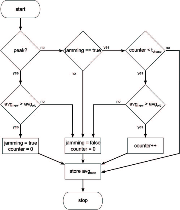
Figure 7 Flowchart of decision control module

$Θ {(x)}_{d e c i s i o n} = ((\frac{1}{s} \sum_{i = n - s - 2}^{n - 2} x_{i} + x_{n} - \bar{x}) - (\frac{1}{s} \sum_{i = n - s - 1}^{n - 1} x_{i} + x_{n} - \bar{x})) (5)$

5.3 Experimental Setup

The experimental setup is shown in Figure 8. We used two sensor nodes for a simple communication between sender and receiver and one node as a jammer. The position of the jammer varies between near sender (position 1), between sender and receiver (position 2) and near receiver (position 3). The data communication and the jamming activity is performed using the 2.4 GHz band on channel 15. To exchange control informations the 868 MHz band is used in parallel. For the experiment we implement two different application for the platform. The first application, called CommApp, periodically sends data packets with a data rate of 250 kbps and a payload of 60 Bytes from sender to receiver. The sending interval is 50 ms. Furthermore, the application periodically reads actual RSSI values from the CC2520 (2.4 GHz) transceiver at every 10 ms and forwards it as input for the jamming detection engine. To analyse the results we forward all important information in CSV format over the UART interface to a logging and control application running on the laptop. Collected data are the current RSSI value, intermediate data of jamming detection, packet delivery rate (PDR), jammer activity, number of received preambles and packets.

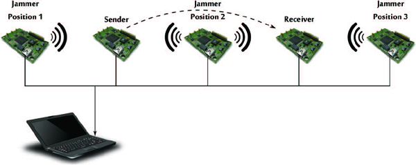
Figure 8 Experimental set-up of jamming scenarios and node positions

The second application, called JammApp, implements three types of jamming, i.e., constant-, periodic- and random jamming. To generate a disturbing signal with CC2520 radio we use a special transmit mode, which send pseudo random data [6]. The state of JammApp can be set to active or inactive and can toggle in periodic or random intervals. Before the activity of the jammer changes, the JammApp sends its state over the control channel via 868 MHz to all sensor nodes. This is needed to be able to check and synchronise the detection results with the actually attack state for evaluation purposes. The actual jamming scenario remains undisturbed by that.

The Figure 9 shows the impact of the communication and jammers on the wireless channel. The first graph (a) is a normal communication between sender and receiver without malicious impact. The graph (b) to (d) illustrate the impact of respective three different types of jamming. To test our detection algorithms we collected data for each scenario over a 30 min time period. For all scenarios following parameters are used:

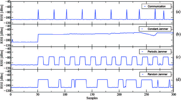
Figure 9 Monitored RSSI values of communication (a), constant jammer (b), periodic jammer (c), random jammer (d)

Clock rate MSP430: 4 MHz

Sample rate: 10 ms

Sliding window of significance analysis: s_sign= 8

Sliding window of peak detection: s_peak= 2

5.4 Implementation Details

Resources used

An overview of the memory consumption is given in Table 2. The table illustrates the size of code (text) and the required memory space (data) of the jamming detection mechanism. The individual functions have been disassembled from the binary files to determine the amount of memory needed. The total text size of the detection engine is 955 bytes only, which is quite acceptable also for sensor nodes. The biggest amount of memory is used for the decision control, which is due to the additionally implemented mechanisms as mentioned above. The space required for the storing values for calculations during runtime is even much lower. We here need 47 bytes for variables only. This gives a total of about 1 KB (1002 bytes) of required memory, which is in a tolerable range even for the limited memory resources of sensor nodes.

Table 2 Static analysis - memory requirements

Function	Memory in [Byte]
	Text	Data
Significance Init() Significance Eval()	33 326	16
PeakDetection Init() PeakDetection Eval()	22 198	17
DecisionControl Init() DecisionControl Eval()	18 358	14
Total	955	47

Online jamming detection tool

To configure the test scenarios we implemented two applications. Both used the virtual serial com port to communicate with the sensor node platform to actively control the scenarios during run-time. The first application, shown on the left side of Figure 10, allows us to set the wireless channel and the transmit power of the radio transceiver of connected sensor node. Furthermore it allows for plotting and storing the current values of detection analysis in real-time. The second application is build for the configuration of the JammApp. Here, the type and activity of the jammer can be set in addition to the pure radio configuration.

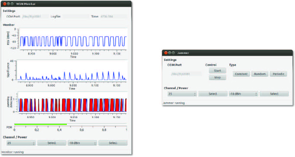
Figure 10 Graphical user interface of remote interface from sensor node (left) and jammer (right) application

Runtime

The time needed to perform the algorithms was measured by gathering required clock cycles. The interrupts of the used timer were configured such that a cycle corresponds to one microsecond in time, at a processor clock rate of 4 MHz. The results are shown in Table 3. A single detection run may require up to 4944 cycles. Thus, a single detection cycle runs approximately 4.9 ms at aclock rate of 4 MHz. If the constant jammer is active, the required time decreases to 4.2 ms (4237 cycles) only. This is due to less processing of data in the decision control, since most of the decision control functionality is only activated when significant changes are detected, i.e. the constant jammer is the best to be recognized very quickly.

Table 3 Captured data and accuracy of jamming detection applying various positions of the jamming device

Experimental results and detection rates

The most crucial goal of each jamming detection method is the effectiveness and accuracy of detecting attacks correctly. Therefore we have separated the number of active jamming phases in relation to the correctly detected jamming phases from the measured data.

First, the attacks of the constant jammer are evaluated. The detection rates for all scenarios with a constant jammer are 100 %. Sender and receiver have thus achieved the same results, although different distances have been tested, i.e., the different positions of the jamming device. That outcome slightly changes when considering the results while the periodic jammer was active. Here not all activities have been recognized correctly and the results are coupled with the distance to the jamming device, as pre-assumed before testing. If the jammer is located in-between sender and receiver at the same distance to both sensor nodes (position 2), then both nodes detect almost all attacks. The maximum measured error rate was 0.18 %. Higher error rates can only be seen at the positions 1 (close to the transmitter) and 3 (near the receiver). At position 1 there is a error rate in contrast to position 3. The reason for this are low deviant RSSI values and due to the simple fact, that transmission is disturbed at the sending device. Thus, a packet may be destroyed while sending already or more important, the sender does not send at all due to already occupied channel. Most MAC protocols of course sample the wireless channel before sending. Nevertheless detection rates of 65.7 % with a minimal increase in the RSSI average of 8.9 dBm can still be obtained. Better results have been measured at position 3. In this scenario, we achieved detection rates of 99.98 % at the receiver and of 91.89 % at the sender respectively. The most difficult jammer to be detected was the random jammer. The rapid change from short to long interfering signals are reflected in the results again. It still reaches values of 84 % to 93.4 %. However, the lower detection results at the receiver and the jammer at position 1 still remain due to low RSSI values returned. Overall, very good results have been achieved in all scenarios given to the fact that not pre-configured jamming is difficult at all, especially in sensor networks. It has been shown that even weak jammers were effectively detected. In a sensor network scenario, all nodes located near to the jammer should be able to detect an attack. Hence, also nodes not affected by the jammer can then inform all other nodes as well as a sink about on-going jamming and take any necessary corrective action, e.g. searching for a suitable other wireless channel.

6 Concluding Remarks

In this paper we have introduced the significance analysis approach as a means to detect jamming in wireless sensor networks in real-time. Since it reacts on changes in the monitored value, here SNR, our approach omits the need for preconfigured values, which are difficult to get and in addition are difficult to use since the impact on the SNR depends on the position of the jammer. We have evaluated the complexity of our approach and shown that in theory the computational effort equals to O(14) and that the memory consumption collapses to storing three integer values. We have evaluated the correctness of the prediction by applying it to real measurements recorded in a jamming experiment.

To provide evidence, we have implemented and tested our jamming detection engine based on the significance analysis on a state of the art sensor network setting. It requires about one kilobyte of code and data memory only. Our jamming detection engine monitors the wireless channel with a sampling rate of 10 ms. It returns a jamming detection decision within less than 5 ms and achieves a detection accuracy in between 84 to 99 percent. It turned out that the obviously best position of jammer is near the receiver, since then the jamming might be overseen by the sending device whereas the receiving one is not able to send an alert message due to ongoing jamming either.

Even though we have proven our approach to be working quite well, there still exist several open questions such as correlation of detection method and used MAC protocols, reaction time to be gained e.g. in case the jamming device slowly increases its transmission power etc. Especially the latter case is of interest for us, since in this case jamming might probably not be detected as a peak in SNR by our approach. In summary, jamming detection methods in general need to be seen as continuous work in progress due to the simple fact that jamming methods and jamming devices will advance too.

References

[1] Wireless Communications: Principles and Practice. Prentice Hall communications engineering and emerging technologies series. Dorling Kindersley, 2009.

[2] J.B.D. Cabrera, C. Gutierrez, and R.K. Mehra. Infrastructures and algorithms for distributed anomaly-based intrusion detection in mobile ad-hoc networks. In Military Communications Conference, MILCOM 2005. IEEE, pages 1831–1837. IEEE, 2006.

[3] Murat Çkiroğlu and Ahmet Turan Özcerit. Jamming detection mechanisms for wireless sensor networks. In Proceedings of the 3rd international conference on Scalable information systems, InfoScale ’08, pages 4: 1–4: 8, ICST, Brussels, Belgium, 2008. ICST.

[4] A. Fragkiadakis, V. Siris, and N. Petroulakis. Anomaly-based intrusion detection algorithms for wireless networks. In 8th International Conference on Wired/Wireless Internet Communications, pages 192–203, Lulea, Sweden, June 2010. Springer.

[5] A. Hamieh and J. Ben-Othman. Detection of jamming attacks in wireless ad hoc networks using error distribution. In Communications, 2009. ICC ’09. IEEE International Conference on, pages 1–6, June 2009.

[6] Texas Instruments. CC2520 DATASHEET –2.4 GHZ IEEE 802.15.4/ZIGBEE RF TRANSCEIVER.

[7] Yu Seung Kim, Frank Mokaya, Eric Chen, and Patrick Tague. All your jammers belong to uslocalization of wireless sensors under jamming attack. In Communications (ICC), 2012 IEEE International Conference on, pages 949–954. IEEE, 2012.

[8] Yee Wei Law, Pieter Hartel, Jerry Hartog den, and Paul Havinga. Link-layer jamming attacks on s-mac. In Proceeedings of the Second European Workshop on Wireless Sensor Networks, 2005, pages 217–225, Los Alamitos, California, 2005. IEEE Computer Society Press.

[9] R. Muraleedharan and L.A. Osadciw. Jamming attack detection and countermeasures in wireless sensor network using ant system. SPIE Defence and Security, Orlando, 2006.

[10] Alejandro Proano and Loukas Lazos. Selective jamming attacks in wireless networks. In Communications (ICC), 2010 IEEE International Conference on, pages 1–6. IEEE, 2010.

[11] K.W. Reese, A. Salem, and G. Dimitoglou. Using standard deviation in signal strength detection to determine jamming in wireless networks. Computers Applications in Industry and Engineering, 2010.

[12] Mario Strasser, Boris Danev, and Srdjan Čapkun. Detection of reactive jamming in sensor networks. ACM Transactions on Sensor Networks (TOSN), 7:16:1–16:29, September 2010.

[13] J. Tang and P. Fan. A RSSI-based cooperative anomaly detection scheme for wireless sensor networks. In International Conference on Wireless Communications, Networking and Mobile Computing, WiCom 2007., pages 2783–2786, Shanghai, 2007.

[14] A. D. Wood, J. A. Stankovic, and Gang Zhou. DEEJAM: Defeating Energy-Efficient Jamming in IEEE 802.15.4-based Wireless Networks. In 4th Annual IEEE Communications Society Conference on Sensor, Mesh and Ad Hoc Communications and Networks, SECON ’07., pages 60–69, 2007.

[15] Wenyuan Xu, Ke Ma, W. Trappe, and Y. Zhang. Jamming sensor networks: attack and defense strategies. Network, IEEE, 20(3): 41–47, May 2006.

[16] Wenyuan Xu, Wade Trappe, Yanyong Zhang, and Timothy Wood. The feasibility of launching and detecting jamming attacks in wireless networks. In Proceedings of the 6th ACM international symposium on Mobile ad hoc networking and computing, MobiHoc, pages 46–57, NY, USA, 2005.

Biographies

Stephan Kornemann received the M.S. degree in information and media technology from Brandenburg University of Technology, Germany, in 2012. From 2010 to 2012 he worked as software tester at Philotech and received his software testing qualification certificate from ISTQB. Since 2012 he is member of the sensor network research group at IHP in Frankfurt (Oder). His current research focuses on intrusion detection systems for wireless sensor networks.

Steffen Ortmann received his diploma in computer science in 2007 and his PhD in engineering by scholarship in 2010. Since 2005 he is active in the sensor network research group of IHP. He has published more than 40 refereed technical articles about reliability, privacy and efficient data processing in wireless sensor networks and medical applications. His current research focuses on mobile wireless sensor networks for tele-medical innovations. He is coordinating the FP7 project StrokeBack and is responsible for medical driven research and the crypto-microcontroller research team within sensor networks group of IHP.

Peter Langendörfer, Professor, holds a diploma and a doctorate degree in computer science. Since 2000 he is with the IHP in Frankfurt (Oder). There, he is leading the sensor networks and mobile middleware group. Since 2012 he has his own chair for security in pervasive systems at the Technical University of Cottbus. He has published more than 100 refereed technical articles, filed ten patents in the security/privacy area and worked as guest editor for many renowned journals e.g. Wireless Communications and Mobile Computing (Wiley). He was chairing International conferences such as WWIC and has served in many TPC for example at Globecom, VTC, ICC and SECON. His research interests include wireless sensor networks and cyber physical systems, especially privacy and security issues.

Alexandros Fragkiadakis received his PhD degree in computer networks from the Department of Electronic and Electrical Engineering of Loughborough University in UK. His thesis focused on active networks using programmable hardware (FPGAs). He has also received an MSc in Digital Communications Systems, awarded with distinction, from the same University. Alexandros obtained his Diploma degree in Electronics from the Technological Educational Institute of Piraeus. He has worked as a Research Associate within the High Speed Networks Group of Loughborough University, in a project involving active networks and field programmable gate arrays. This project was funded by the Engineering and Physical Sciences Research Council, a British Government’s leading funding agency for research and training in engineering and the physical sciences. Alexandros joined the Telecommunications and Networks Laboratory of the Institute of Computer Science of the Foundation for Research and Technology-Hellas in November 2008. His research interests include wireless networks, intrusion and anomaly detection in wireless networks, reprogrammable devices, cloud computing, open source architectures, cognitive radio networks, wireless sensor networks.