Study on Estimating Buffer Overflow Probabilities in High-Speed Communication Networks

Received: January 2015; Accepted: 18 February 2015;
Publication: 3 April 2015

Izabella Lokshina

• Department of Management, Marketing and Information Systems SUNY–Oneonta, NY 13820, USA Izabella.Lokshina@oneonta.edu

---

Abstract

The paper recommends new methods to estimate effectively the probabilities of buffer overflow in high-speed communication networks. The frequency of buffer overflow in queuing system is very small; therefore the overflow is defined as rare event and can be estimated using rare event simulation with continuous-time Markov chains. First, a two-node queuing system is considered and the buffer overflow at the second node is studied. Two efficient rare event simulation algorithms, based on the Importance sampling and Cross-entropy methods, are developed and applied to accelerate the buffer overflow simulation with Markov chain modeling. Then, the buffer overflow in self-similar queuing system is studied and the simulations with long-range dependent self-similar traffic source models are conducted. A new efficient simulation algorithm, based on the RESTART method with limited relative error technique, is developed and applied to accelerate the buffer overflow simulation with SSM/M/1/B modeling using different parameters of arrival processes and different buffer sizes. Numerical examples and simulation results are provided for all methods to estimate the probabilities of buffer overflow, proposed in this paper.

---

Keywords

• high-speed communication networks, estimating probability of buffer overflow
• two-node queuing system with feedback
• Importance sampling method
• Cross-entropy method
• self-similar queuing system
• RESTART method with limited relative error technique

---

1 Introduction

Overflows in high-speed communication networks are uncommon and defined as rare events. The frequency of rare events is very small, e.g. 1^-6 or less; however, rare event probability can be used to simulate, estimate and analyze many queuing system characteristics. Queuing systems are appropriate reference models being used in different mehodologies and techniques to accelerate rare event simulation in high-speed communications networks. Estimation of rare event probability using Monte Carlo simulation requires a very long computing time and cannot easily be implemented [2, 4, 19]. Lately two basic methods of the rare event simulation were developed based on cross-entropy approach that can be applied to a wide range of optimization tasks [6, 9, 10]:

• Splitting of the sample path that for to reach definite intermediate level between the starting level and rare event [5]; and
• Importance Sampling (IS) generation [3].

The Probability Density Function (PDF) is used in the IS approach as a rare event evaluation measure, which can be compared and changed based on the likelihood ratio of the less rare event PDF [17].

One of the rare event simulation objectives is estimating total network population overflow. Exact large deviation analysis leading to asymptotically efficient change of measure is rather difficult. Instead, heuristic change of measure is proposed, which interchanges the arrival rate to the first queue and the slowest service rate. Similar change of measure is suggested based on time reversal arguments. However, analysis shows that the IS estimator based on this change of measure is not necessarily asymptotically efficient. In fact, it has an infinite variance in some parameter regions [10].

Another rare event simulation objective is estimating buffer overflow observed at individual network node. This objective is the purpose of our study. If the node of concern is a bottleneck relative to all preceding nodes, then asymptotically efficient exponential change of measure can be obtained by interchanging the arrival rate and the service rate at this particular node; and the service rates at all other nodes are kept unchanged [11–12].

However, this change of measure is not asymptotically efficient when overflow of buffer at the consequent node is considered. Effective bandwidth is used to derive heuristics for efficient feed-forward discrete-time queuing network simulation. This class of networks essentially resembles feed-forward fluid-flow networks. The analogous approach to continuous-time queuing networks has not yet been introduced even for Markov chains.

Initially, two-node queuing systems are considered in this paper; and the event of buffer overflow at the second node is studied. Discrete-Time Markov Chain (DTMC) with its regular structure is highly efficient model used for performance evaluation of the queuing system. On one hand, the states are easily arranged as a grid in DTMC (with as many dimensions as the number of queues). On the other hand, any transition in DTMC corresponds to a particular elementary event at one of the queues (e.g., arrival or service completion). These events are known as transition events, and they are defined separately from the states; i.e., there is only one transition event for a service completion at a given queue, and this particular transition event corresponds to a transition out of each state in the DTMC while this particular queue is non-empty [13, 16].

However, not all transition events are enabled in every state. For example, the service completion event of the particular queue is not possible in a state where the queue is empty.

In this paper we propose a new simulation method based on Markov Additive Continuous-Time Process (MAP) modeling. We develop and apply Importance sampling algorithm with exponential tilting of the unbiased PDF estimation to the appropriate MAP representation, which let us estimate effectively the probability of buffer overflow at the second node. Unlike several heuristic changes of measure described in the literature, the derived change of measure depends on the content of the first buffer.

When the first buffer is finite, we confirm that the proposed simulation procedure yields the estimation with a relative error that is bound independent of the buffer overflow level. This result is much stronger than the asymptotic efficiency, which cannot be observed with other known methods.

When the first buffer is infinite, we propose a natural extension of change of measure for finite buffer case. Applying the orthogonal polynomial model we obtain two types of simulation behavior. When the second buffer is a bottleneck, we confirm once more that simulation yields the estimation with a relative error that is bound independent of the buffer overflow level. However, when the first buffer is a bottleneck, the simulation results prove that the relative error is asymptotic and linearly bound to the buffer overflow level.

Finally, long-range dependent self-similar queuing systems are considered in this paper; and the event of buffer overflow is studied. We propose a new steady-state simulation method, based on SSM/M/1/B modeling.

We develop and apply RESTART with Limited Relative Error (LRE) algorithm, which let us estimate effectively the probability of buffer overflow in a long-range dependent self-similar queuing system with different parameters of arrival processes and different buffer sizes.

2 Estimating Probability of Buffer Overflow in Continuous Time Queueing Systems

Markov additive continuous-time process is a stochastic process (J_t, Z_t), where (J_t) is Markov chain with the denumerable state space, and (Z_t) has stationary and independent increments during the time intervals when (J_t) is in any given state. That is, if given J_t has not changed in the interval (t₁, t₂), then for any t₁<s₁<…<s_n<t₂, the increments $Z_{s_2}-Z_{s_1},\dots \text{},Z_{s_n}-Z_{s_{n-1}}$ are mutually independent, and the total increment during the interval [t₁, t₂] depends on t₁ and t₂ only through the difference t₂ - t₁.

Moreover, the transition from state i to state j (J_t) has a certain probability (depending only on i and j) of triggering the transition of (Z_t) at the same time. The size of the transition in the process (Z_t) has fixed distribution, which depends only on i and j.

Markov additive continuous-time process (J_t, Z_t) is characterized by the family of the matrices (M_t(s), t ≥ 0), where (i,j)-th element of M_t (s) is (1),

$${[M_t(s)]}_{ij}=E_i[e^{s(Z_t-Z_0)}{I}_{\{J_t=j\}}](1)$$

where E_i, denote the expectation operator given to the initial MAP state J₀ = i. Let us notice that M_t(·) is a generalization of the moment generating function for the ordinary random variables, as shown in (2).

$$\begin{array}{l}{\text{E}}_i[e^{s(Z_{t+h}-Z_0)}{I}_{\{J_{t+h}=j\}}]=\\ ={\displaystyle \sum _k{\text{E}}_i[e^{s(Z_{t+h}-Z_0)}{I}_{\{J_t=k\}}{I}_{\{J_{t+h}=j\}}]}\\ ={\displaystyle \sum _k{\text{E}}_i}[e^{s(Z_t-Z_0)}{I}_{\{J_t=k\}}]{\text{E}}_i[e^{s(Z_{t+h}-Z_t)}{I}_{\{J_{t+j}=j\}}|J_t=k](2)\\ ={\displaystyle \sum _k{[M_t(s)]}_{ik}{\text{E}}_k[e^{s(Z_h-Z_0)}I\{J_{h=j}\}]}\end{array}$$

Consequently, if for all k and j (3) can be defined,

$${[A(s)]}_{kj}:=\underset{h\downarrow 0}{\lim }\frac{1}{h}{E}_k[e^{s(Z_h-Z_0)}{I}_{J_h=j}-{\delta }_{kj}](3)$$

where δ is usual notation of Dirac, then (4) can be easily obtained,

$$\frac{d}{dt}{M}_t(s)=M_t(s)A(s),t\ge 0(4)$$

with M₀(s) = I (the identity matrix). It is true as soon as (5) is true.

$$M_t(s)=e^{tA(s)},t\ge 0(5)$$

The matrix A(s) is known as the MAP (infinitesimal) generator.

Let us consider a simple Markov chain that consists of two queues in tandem. The calls arrive to the first queue (e.g., buffer) according to Poisson process with the rate λ. The departure time is exponentially distributed with the rate μ₁. The calls that leave the first queue enter the second queue. The departure time has an exponential distribution with the rate μ₂.

The queuing system stability is assumed, i.e. λ < min {μ₁, μ₂}. The size of the first buffer may be finite or infinite; in fact, let us consider both cases. Let X_t and Y_t denote the number of the calls in the first and the second queues at the time t, respectively. Let P_i denote the probability measure under which (X_t) starts from i at the time 0 (i.e., X₀ = i, i ≥ 0); and let E_i, denote the corresponding expectation operator.

Assuming that the second buffer is initially non-empty, say, Y₀ = 1, the probability that, starting from (X₀, Y₀) = (i, 1), content of the second buffer hits some high level L ∈ N before hitting 0, can be estimated. This probability is noted by γ_i, and referred to it as the second buffer overflow probability, given that the initial number of calls in the first queue is i.

2.1 Rare Event Simulation with Markov Chain Modeling

Let us consider the IS approach for the rare event simulation, where the probability density function is used as the measure of rare event evaluation, which is compared and changed with the likelihood ratio of the probability density function of a less rare event. First, let us determine the rare event. Let X = (X₁, … , X_N) be a random vector, which values belong to the certain state space χ. Let { f(·, v)} be the family of the probability density functions on χ, with respect to some base measure υ. Here v is a real-valued parameter (vector). Then, for any measurable function H is obtained as (6).

$$\text{E}[H(\text{X}){\displaystyle \int H(\text{x})f(\text{x};\text{v})\upsilon (d\text{x})}](6)$$

In many cases f is often called the Probability Mass Function (PMF), but in this paper the generic term density, or the Probability Density Function (PDF), is used. Let S be some real function on χ . The probability that S(X) is greater than some real number γ, under F(·;u) can be defined. Therefore, probability can be written as (7),

$$l={\text{P}}_{\text{u}}(S(\text{X})\ge \gamma )={\text{E}}_{\text{u}}[I_{\{S(\text{X})\ge \gamma \}}](7)$$

where $I_{\{S(\text{X})\ge \gamma \}}$ is the indicator function. If this probability is very small, like 10^-6 or less, then $\{S(\text{X})\ge \gamma \}$ is a rare event. The simplest way to estimate l is to use the basic Monte Carlo simulation. Draw a random sample X₁,…, X_N from f(·;u), and use (8) as the unbiased estimator of l.

$$\frac{1}{N}{\displaystyle \sum _{i=1}^N{I}_{\{S({\text{X}}_i)\ge \gamma \}}}(8)$$

However, it poses serious problems when $\{S(\text{X})\ge \gamma \}$ is a rare event. In that case a large simulation effort is required in order to estimate l accurately. An alternative is based on the IS. Take a random sample X₁,…, X_N from the IS density g on χ, and evaluate l using the unbiased estimator, called the likelihood ratio estimator (9).

$$\widehat{l}=\frac{1}{N}{\displaystyle \sum _{i=1}^N{I}_{\{S({\text{X}}_i)\ge \gamma \}}}\frac{f({\text{X}}_i;\text{u})}{\text{g}({\text{X}}_i)}(9)$$

It is well known that the optimal way to estimate l is to use the change of the measure with the density (10)

$${\text{g}}^{*}(\text{x})=\frac{I_{\{S(\text{X})\ge \gamma \}}f(\text{x};\text{u})}{l}(10)$$

Specifically, applying this change of the measure to (9), (11) can be obtained for all i.

$$I_{\{S({\text{X}}_i)\ge \gamma \}}\frac{f({\text{X}}_i;\text{u})}{{\text{g}}^{*}({\text{X}}_i)}=l(11)$$

In other words, the estimator (9) has a zero variance, and only N = 1 sample need to be produced. The obvious difficulty is, of course, that the g* depends on the unknown parameter l. Moreover, one often wishes to choose this g from the density family {f(·, v). Now the plan is to choose the tilting parameter v, such that the distance between the densities g* and f(·, v) is minimal.

A particular suitable measure of the distance between two densities g and f is the Kullback-Leibler distance, which is defined in (12).

$$\begin{array}{l}D\left(\text{g},f\right)={\text{E}}_{\text{g}}[\ln \frac{\text{g}(\text{X})}{f(\text{X})}]\\ ={\displaystyle \int \text{g}(\text{x})\ln \text{g}(\text{x})\upsilon (d\text{x})-{\displaystyle \int \text{g}(\text{x})\ln f(\text{x})\upsilon (d\text{x})}}(12)\end{array}$$

Therefore, minimizing the Kullback-Leibler distance between g in (11) and f(·,v) is the same as choosing v, such that $-{\displaystyle \int \text{g}(\text{x})\text{In}}f(\text{x};\text{v})\upsilon (d\text{x})$ is minimized, or equally, such that $-{\displaystyle \int \text{g}(\text{x})\text{In}}f(\text{x};\text{v})\upsilon (d\text{x})$ is maximized. Formally, it can be written as (13).

$$\underset{\text{v}}{\max }D(v)=\underset{\text{v}}{\max }{\displaystyle \int \text{g}(\text{x})}Inf(\text{x};\text{v})\upsilon (d\text{x})(13)$$

Applying g from (10) to (13) as the substitution, the following optimization program can be obtained as (14).

$$\begin{array}{l}\underset{\text{v}}{\max }D(\text{v})=\underset{\text{v}}{\max }{\displaystyle \int \frac{I_{\{S(\text{X})\ge \gamma \}}f(\text{x};\text{u})}{l}}\text{In}f(\text{x};\text{v})\upsilon (d\text{x})\\ =\underset{\text{v}}{\max }{\text{E}}_{\text{u}}[I_{\{S(\text{X})\ge \gamma \}}\text{In}f(\text{X};\text{v})](14)\end{array}$$

Using the IS again, with the change of measure f(·;w), (14) can be re-written into (15),

$$\underset{\text{v}}{\max }D(\text{v})=\underset{\text{v}}{\max }{\text{E}}_{\text{w}}[I_{\{S(\text{X})\ge \gamma \}}W(\text{X};\text{u},\text{w})\text{In}f(\text{X};\text{v})](15)$$

for any tilting parameter {w}, where the likelihood ratio at x between f(·;u) and f(·;w) is W. This can be presented according to (16).

$$W(\text{x};\text{u};\text{w})=\frac{f(\text{x};\text{u})}{f(\text{x};\text{w})}(16)$$

The basic idea of the IS method regarding rare event is to accelerate its frequency with iterative tilting the unbiased estimation of the probability density function to appropriate MAP representation.

The acceleration of conditional probability of rare event X₁ with one-parameter function f(x) is shown in Figure 1. The conditional probability of rare event ${\text{P}}_{\text{f}}\{\text{x}>{\text{X}}_1\}$ is changing with conditional probability of $\text{g}(\text{x})-{\text{P}}_{\text{g}}\{\text{x}>{\text{X}}_1\}$.

.

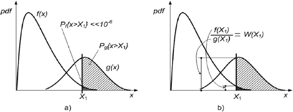
Figure 1 Conditional probability of rare event P_f{x > X₁} – (a); and its acceleration with likelihood ratio W(X₁) – (b).

At each iteration of the IS simulation, N independent samples are generated, which distribution g(x) can be evaluated with the likelihood ratio W(X₁). The optimal solution for (15) can be written as (17).

$${\text{v}}^{*}=\underset{\text{v}}{\arg \max }{\text{E}}_{\text{w}}[I_{\{S(\text{X})\ge \gamma \}}W(\text{X};\text{u},\text{w})\text{ln}f(\text{X};\text{v})](17)$$

It can be obtained by solving the following stochastic program, which can be considered as a stochastic counterpart of (15) and written according to (18),

$$\underset{\text{v}}{\max }\widehat{D}(\text{v})=\underset{\text{v}}{\max }\frac{1}{N}{\displaystyle \sum _{i=1}^N{I}_{\{S(\text{X})\ge \gamma \}}}W(X_i;u,w)lnf(X_i;v)(18)$$

where X₁,…,X_N is a random sample from f(·;w).

The solution for (18) can be obtained by solving the following system of equations with respect to v in (19),

$$\frac{1}{N}{\displaystyle \sum _{i=1}^N{I}_{\{S({\text{X}}_i)\ge \gamma \}}}W({\text{X}}_i;\text{u},\text{w})\nabla \text{ln}f({\text{X}}_i;\text{v})=0(19)$$

where the gradient is defined regarding v.

This confirms the expectation that the differentiation operators and the function $\widehat{D}$ can be interchanged in (18) with respect to v. The advantage of this approach is in the fact that often the solution of (19) can be calculated analytically. In particular, this happens when the random variable distributions belong to the natural exponential family. The cross-entropy program (19) is useful only when the probability of the target event {S(X) ≥ γ} is not too small, say 1 ≥ 10^-5.

Then, above program is useful in terms of potentially more accurate estimator determination. However, in a rare event context, (say, 1 ≥ 10^-6), the program (19) is useless to rarity of events {S(X_i) ≥ γ}, because the random variables $I_{\{S({\text{X}}_i)\ge \gamma \}},\text{i}=l,\mathrm{...},\text{N}$ and the associated derivatives of $\widehat{D}(\text{v})$ vanish with high probability, as given in the right-hand side of (19), for reasonable sizes of N.

2.2 Exponential Change of Measure

Let us initially think that the first buffer has a finite capacity N. In this case the state space of the driving process (X_t) is finite in {0,…,N}. Let us consider Markov additive continuous-time process (X_t, Z_t). To create a corresponding MAP generator (i.e., matrix A(s) in (5)), the infinitesimal expectations ${\text{E}}_i[e^{s(Z_h-Z_0)}{I}_{\{X_h = j\}}-{\delta }_{ij}]$ as $\text{h}\downarrow 0$ for all i, j in {0,…,N} have to be determined, where Z₀ = l and δ_ij = 0 for j ≠ i.

For instance, since the downward transition of (X_t) leads to the upward transition of (Z_t), (20) is used for i = l,…, N, as $\text{h}\downarrow 0$.

$$\begin{array}{l}{\text{E}}_i[e^{s(Z_h-Z_0)}{I}_{\{X_h = i-1\}}-{\delta }_{i,i-1}]=\\ ={\text{E}}_i[e^{s(Z_h-Z_0)}|X_h=i-1]{\text{P}}_i(X_h=i-1)=\\ =e^s({\mu }_{1}h+O(h))={\mu }_{1}h{e}^s+o(h)(20)\end{array}$$

Therefore, the (i, i-l)-th element of the matrix A(s) exists and is equal to ${\text{μ}}_1{\text{e}}^{\text{s}}$. Other elements of the matrix A(s) can be defined similarly. Consequently, (5) holds with A(s) for Markov additive continuous-time process (X_t, Z_t) with the given (N + l, N + l)-tridiagonal matrix (21).

$${\text{G}}_N(s)=\left(\begin{array}{cccc}-\lambda -{\mu }_2+{\mu }_2{e}^{-s}& \lambda & & \\ {\mu }_1{e}^s& -\lambda -{\mu }_1-{\mu }_2+{\mu }_2{e}^{-s}& \lambda & \\ & \ddots & \ddots & \ddots \\ & & {\mu }_1{e}^s& -{\mu }_1-{\mu }_2+{\mu }_2{e}^{-s}\end{array}\right)(21)$$

Let us note that the MAP generator G_N(s) is now equal to the matrix (22).

$${\widehat{\text{Q}}}^{(n)}(u)=\left(\begin{array}{cccc}-\lambda -{\mu }_2+{\mu }_{2}u& \lambda & & \\ {\mu }_1/u& -\lambda -{\mu }_1-{\mu }_2+{\mu }_{2}u& \lambda & \\ & \ddots & \ddots & \ddots \\ & & {\mu }_1/u& -{\mu }_1-{\mu }_2+{\mu }_2{e}^{-s}\end{array}\right)(22)$$

Next, the change of the measure based on the family of the matrices G_N(s) is defined. For any s ≥ 0, k_N(s): = log(sp(M_t(s)))/t has to be defined, where sp(M_t(s)) denotes the spectral radius (or, the maximum Eigen value) of M_t(s). Using (5) k_N(s) can be identified as the largest positive Eigen value of G_N(s). Let w(s) = {w_k(s),0 ≤ k ≤ N} represent the correspondent right-eigenvector.

When the first buffer has the infinite capacity, the process (X_t, Z_t) is still Markov additive continuous-time process, but the state space for Markov process (X_t) is now infinite. Equation (5) is still used, but A(s) is now given by the infinite-dimensional tri-diagonal matrix (23).

$$\text{G}(s)=\left(\begin{array}{cccc}-\lambda -{\mu }_2+{\mu }_2{e}^{-s}& \lambda & & \\ {\mu }_1{e}^s& -\lambda -{\mu }_1-{\mu }_2+{\mu }_2{e}^{-s}& \lambda & \\ & \ddots & \ddots & \ddots \\ & & & \end{array}\right)(23)$$

Let us note that the MAP generator G(s) is now equal to the infinite tri-diagonal matrix (24).

$$\text{Q}(u)=\left(\begin{array}{cccc}-\lambda -{\mu }_2+{\mu }_{2}u& \lambda & & \\ {\mu }_1/u& -\lambda -{\mu }_1-{\mu }_2+{\mu }_{2}u& \lambda & \\ & \ddots & \ddots & \ddots \\ & & & \end{array}\right)(24)$$

2.3 Importance Sampling Algorithm and Simulation Results

The Markovian network that consists of tandem queues with feedback is shown in Figure 2 and used as a simulation example, with the entry parameters follow: λ₁ = λ₂, μ₁ = μ₂ = 6, p = 0.5.

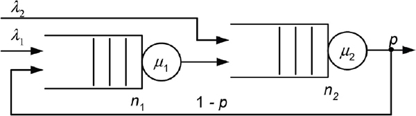
Figure 2 Two-node queuing network with feedback.

The Importance Sampling (IS) algorithm to accelerate rare event simulation with Markov chain modeling in high-speed communication networks is suggested in this paper. It consists of the following six steps provided below.

Algorithm 1 Importance sampling simulation method

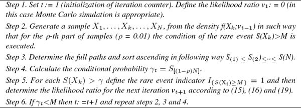
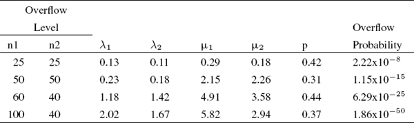
The simulation results for Poisson distribution and fixed numbers of calls n₁ and n₂, for four different overflow cases are provided in Table 1. As could be seen, the overflow probability exponentially decreases with increase of the fixed number of calls in queues n₁ and n₂. The exponential behavior depends more on the number n₁.

Table 1 Simulation results

2.4 Cross-Entropy Algorithm and Simulation Results

The Cross-entropy algorithm to accelerate rare event simulation with Markov chain modeling in high-speed communication networks is suggested in this paper. The idea is to introduce a sequence of reference parameters {v_t, t ≥ 0} and a sequence of the levels {γ_t, t ≥ 1}, and iterate in both γ_t and v_t.

The initialization is done with choosing a not very smallp, say ρ = 10^-2, and defining v₀ = u. Next, we let γ₁ (γ₁ < γ) be such that under the original density f(x; u), the probability 1₁ = E_u [I_{{s(x)≥ γ1}}] is at least ρ.

After, let v₁ be the optimal cross-entropy reference parameter to estimate l₁, and repeat the last two steps iteratively with the purpose to estimate the pair {l, v*}. In other words, the iteration of the algorithm consists of two main phases. In the first phase γ_t is updated, in the second phase v_t is updated. Particularly, starting with v₀ = u, the subsequent γ_t and v_t are obtained as described below.

Phase 1 includes adaptive update of γ_t. For a fixed v_t-1, let γ_t be a (1-ρ)-quintile of S(X) under v_t-1. That is, γ_t satisfies (25) and (26).

$${\text{P}}_{v_{t-1}}(S(\text{X})\ge {\gamma }_t)={\text{E}}_{\text{u}}[I_{\{S(\text{X})\ge \gamma \}}](25)$$

$${\text{P}}_{v_{t-1}}(S(\text{X})\le {\gamma }_t)\ge 1-\rho (26)$$

where X∼f(·; v_t-1). The simple estimator ${\widehat{\gamma }}_t$ of γ_t can be obtained by drawing a random sample X₁, …, X_N from f(· ; v_t-1), calculating the performances S(X_i) for all i, ordering them from the smallest to the biggest: S₍₁₎ ≤ … ≤ S_(N) and finally, evaluating the (1 - ρ) sample quintile as (27).

$${\widehat{\gamma }}_t=S_{[(1-\rho )N]}(27)$$

Let us note that S_(j) is called j^-th order-statistic of the sequence S(X₁),…,S(X_N). Let us note also that ${\widehat{\gamma }}_t$ is chosen such that the event $\{S(\text{X})\ge {\widehat{\gamma }}_t\}$ is not too rare (it has a probability of around ρ), and therefore, the reference parameter updated with a procedure such as (27) is not void of the meaning.

Phase 2 contains adaptive update of v_t. For fixed γ_t and v_t-1, let us derive v_t from the solution of the following cross-entropy program according to (28).

$$\underset{\text{v}}{\max }D(\text{v})=\underset{\text{v}}{\max }{\text{E}}_{{\text{v}}_{\text{t-1}}}[I_{\{S(X)\ge \gamma \}}W(\text{X};\text{u},{\text{v}}_{t-1})\text{In}f(\text{X};\text{v})](28)$$

The stochastic counterpart of (28) is shown as follows: for fixed ${\widehat{\gamma }}_t$ and ${\widehat{v}}_{t-1}$, derive ${\widehat{v}}_t$, from the solution of the program according to (29).

$$\underset{\text{v}}{\max }\widehat{D}(\text{v})=\underset{\text{v}}{\max }\frac{1}{N}{\displaystyle \sum _{i=1}^N{I}_{\{S({\text{X}}_i)\ge {\widehat{\gamma }}_t\}}}W({\text{X}}_i;\text{u},{\widehat{\text{v}}}_{t-1})\text{ln}f({\text{X}}_i;\text{v})(29)$$

Therefore, at the first iteration starting with ${\widehat{v}}_1$, the target event is artificially made less rare with temporarily use of the level ${\widehat{\gamma }}_1$, which is chosen smaller than γ that for to get a good estimate for ${\widehat{v}}_1$.

The value ${\widehat{v}}_1$ obtained in this way will make the event {S(X)≥ γ} less rare in the next iteration, so the value ${\widehat{\gamma }}_2$ can be used in the next iteration, which is closer to γ itself.

The algorithm terminates when the level is reached at some iteration t, which is at least γ and after the original value of γ can be used without getting too few samples. As mentioned before, the optimal solution of (28) and (29) can be often obtained analytically, in particular when f(x; v) belongs to the natural exponential family.

The above rationale results are placed in the multi-level Cross-entropy algorithm for accelerated rare event simulation with Markov chain modeling in high-speed communication networks. This efficient algorithm consists of the following five steps provided below.

Algorithm 2 Multi-Level Cross-Entropy Simulation Method

$$\widehat{l}=\frac{1}{N}{\displaystyle \sum _{i=1}^{N_1}{I}_{\{S({\text{X}}_i)\ge \gamma \}}}W({\text{X}}_i;\text{u},{\widehat{v}}_T)(30)$$

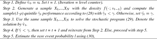
where T denotes the final number of iterations, or number of the levels used.

As a simulation example, let us apply this efficient algorithm to a similar tandem queue with feedback as was given in Figure 2, but at this time with the following entry parameters: λ = 0.2; μ₁ = 0.8; μ₂ = 0.2; p = 0.5.

Table 2 Simulation results

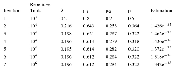
The simulation results for generating N = 10,000 samples are shown in Table 2. As could be seen, overflow is obtained when there are j = 6 iterations. The accuracy increases up to N = 1,000,000 in the seventh iteration, and the overflow probability is obtained equal to ${\widehat{\ell }}_{IS}=1.342{\text{e}}^{\text{-15}}$.

3 Estimating Probability of Buffer Overflow in Self-Similar Queuing Systems

Recent studies of high-speed communication network traffic have clearly shown that teletraffic (technical term, identifying all phenomena of transport and control of information within the high-speed communication networks) exhibits long-range dependent self-similar properties over a wide range of time scales. Therefore, self-similar queuing systems are appropriate reference models being also used in different methodologies and techniques to accelerate rare event simulation in high-speed communication networks [13].

Long-range dependent self-similar teletraffic is usually observed in LAN and WAN, where superposition of strictly independent alternating ON/OFF traffic models, whose ON- or OFF-periods have heavy-tailed distributions with infinite variance, can be used to model aggregate queuing network traffic that exhibits long-range dependent self-similar behavior, typical for measured LAN traffic over a wide range of time scales [14, 18].

Long-range dependent self-similar teletraffic is also observed in ATM networks: when arriving at an ATM buffer, it results in a heavy-tailed buffer occupancy distribution, and a buffer cell loss probability decreases with the buffer size not exponentially, like in traditional Markovian models, but hyperbolically [16, 18].

Furthermore, long-range dependent self-similar teletraffic is observed in the Internet as many characteristics can be modeled using heavy-tailed distributions, including the distributions of traffic times, user requests for documents, and document sizes. In IP with TCP self-similar queuing networks the transfer of files or messages shows that the reliable transmission and flow control mechanisms serve to maintain long range dependent structure included by heavy-tailed file size distributions [1].

Long-range dependent self-similar video traffic provides possibility for developing models for Variable Bit Rate (VBR) video traffic using heavy-tailed distributions [16, 18]. Therefore; we can clearly see that impact of self-similar models on the queuing and network performance is very significant.

The properties of long-range dependent self-similar teletraffic are very different from properties of traditional models based on Poisson, Markov-modulated Poisson, and related processes. More specifically, while tails of the queue length distributions in traditional teletraffic models decrease exponentially, those of long-range dependent self-similar teletraffic models decrease much slower.

Therefore, the use of traditional models in high-speed communication networks characterized by long-range dependent self-similar processes can lead to incorrect conclusions about the queuing and network performance. Traditional models can lead to over-estimation of the queuing and network performance, insufficient allocation of communication and data processing resources, and consequently difficulties in ensuring the QoS.

Self-similarity can be classified into two types: deterministic and stochastic. In the first type, deterministic self-similarity, a mathematical object is assumed to be self-similar (or fractal) if it can be decomposed into smaller copies of itself. That is, deterministic self-similarity is a property, in which the structure of the whole is contained in its parts [14, 18].

This work is focused on stochastic self-similarity. In that case, probabilistic properties of self-similar processes remain unchanged or invariant when the process is viewed at different time scales. This is in contrast to Poisson processes that lose their burstiness and flatten out when time scales are changed [18].

However, the time series of self-similar processes exhibit burstiness over a wide range of time scales. Self-similarity can statistically describe teletraffic that is bursty on many time scales [14].

One can distinguish two types of stochastic self-similarity. A continuous-time stochastic process Y_t, is strictly self-similar with a self-similarity parameter H (1/2 < H < 1), if Y_ct, and c^HY_t (the rescaled process with time scale ct) have identical finite-dimensional probability for any positive time stretching factor c. This definition, in a sense of probability distribution, is quite different from that of the second-order self-similar process, observed at the mean, variance and autocorrelation levels [14].

The process X is asymptotically second-order self-similar with 0.5 < H < 1, if for each k large enough ${\rho }_k^{(m)}\to {\rho }_k$, as $m\to \infty$, where ${\rho }_k=\text{E}[(X_i-\mu )(X_{i+k}-\mu )]/{\sigma }^2.$

In this work the exact or asymptotic self-similar processes are used in an interchangeable manner, which refers to the tail behavior of the autocorrelations [14, 18].

3.1 Long-Range Dependent Self-Similar Processes

We have to say that the most striking feature of some second-order self-similar processes is that the accumulative functions of the aggregated processes do not degenerate with the non-overlapping batch size m increasing to infinity. Such processes are known as Long-Range Dependent (LRD) processes [1, 14, 18].

This is in contrast to traditional processes used in modeling high-speed communication network traffic, all of which include the property that the accumulative functions of their aggregated processes degenerate as the non-overlapping batch size m increasing to infinity, i.e., ${\rho }_k^{(m)}\to 0$ or ${\rho }_k^{(m)}=0(|k|>0)$ for m > 1. The equivalent definition of long-range dependence is given as (31).

$${\displaystyle \sum _{k=-\infty }^{\infty }{\rho }_k}=\infty (31)$$

Another definition of LRD is presented as (32),

$${\rho }_k~L(t)k^{-(2-2H)}\text{},\text{as}\text{k}\to \infty (32)$$

where 1/2 < H <1 and L(·) slowly varies at infinity, i.e. for all x > 0 it could be determined as (33).

$$\underset{t\to \infty }{\lim }\frac{L(xt)}{L(t)}=1(33)$$

The Hurst parameter H characterizes the relation in (32), which specifies the form of the tail of the accumulative function. One can show that is true for 1/2 < H < 1, as given in (34).

$${\rho }_k=\frac{1}{2}\left[{(k+1)}^{2H}-2k^{2H}+{(k-1)}^{2H}\right](34)$$

For 0 < H < 1/2 the process is Short-Range Dependent (SRD) and could be presented as (35).

$${\displaystyle \sum _{k = -\infty }^{\infty }{\rho }_k}=0(35)$$

For H = 1 all autocorrelation coefficients are equal to one, no matter how far apart in time the sequences are. This case has no practical importance in real high-speed communication network traffic modeling. If H > 1, then (36) is true.

$${\rho }_k=\{\text{}\begin{array}{cc}1& \text{for}k=0\\ \frac{1}{2}{k}^{2H}g(k^{-1})& \text{for}k>0\end{array}(36)$$

where

$$\text{g}(x)={(1+x)}^{2H}-2+{(1-x)}^{2H}(37)$$

One can see that $g(x)\to \infty$ as H > 1. If 0 < H < 1 and H ≠ 1/2, then the first non-zero term in the Taylor expansion of g(x) is equal to $2H(2H-1)x^2.$ Therefore, (38) is true.

$${\rho }_k/(H(2H-1)k^{2H-2})\to 1,\text{as}k\to \infty (38)$$

In the frequency domain, an essentially equivalent definition of LRD for a process X with given spectral density (39),

$$f(\lambda )=\frac{{\sigma }^2}{2\pi }{\displaystyle \sum _{k = -0}^{\infty }{\rho }_k}{e}^{ik\lambda }(39)$$

is that in the case of LRD processes, this function is required to satisfy the following property (40),

$$f(\lambda )~c_{f_1}{\lambda }^{-\gamma },\text{as}\lambda \to 0(40)$$

where $c_{f_1}$ is a positive constant and 0 < γ < 1, γ =2H - 1 < 1. As a result, LRD manifests itself in the spectral density that obeys a power-law in the vicinity of the origin. This implies that $f(0)={\displaystyle {\sum }_k{\rho }_k=\infty }$. Consequently, it requires a spectral density, which tends to +∞ as the frequency λ approaches 0.

For a Fractional Gaussian Noise (FGN) process, the spectral density f(λ, H) is given by (41),

$$f(\lambda ,H)=2c_f(1-\cos (\lambda ))B(\lambda ,H)(41)$$

with 0 < H < 1 and − π ≤ λ ≤ π, where (42) is true,

$$\begin{array}{l}{c}_f={\sigma }^2{(2\pi )}^{-1}\sin (\pi \text{}H)\Gamma (2H+1)\hfill \\ B(\lambda ,H)={\displaystyle \sum _{k = -\infty }^{\infty }|} 2\pi k+\lambda {|}^{-2H-1}\hfill \end{array}(42)$$

and σ² = Var[X_k] and Γ (·) is the gamma function. The spectral density f(λ, H) in (41) complies with a power-law at the origin, as shown in (43),

$$f(\lambda ,H)\to c_f{\lambda }^{1-2H},\text{as}\lambda \to 0(43)$$

where 1/2 < H < 1.

3.2 Steady-State Simulation with SSM/M/1/B Modeling

As we have previously accepted, there is a significant difference in the queuing and network performance between traditional models of teletraffic, such as Poisson processes and Markovian processes, and those exhibiting long-range dependent self-similar behavior. More specifically, while tails of the queue length distributions in traditional models of high-speed communication network traffic decrease exponentially, those of self-similar traffic models decrease much slower (14]; [18]).

Let us consider the potential impacts of traffic characteristics, including the effects of long-range dependent self-similar behavior on queuing and network performance, protocol analysis, and network congestion controls. Steady-state simulation of long-range dependent self-similar queuing system includes:

• Generation of long-range dependent self-similar traffic [14, 18];
• Simulation of long-range dependent self-similar queuing process [14]; and
• Simulation of the overflow probability [14, 15].

This can be demonstrated with the buffer overflow simulation in SSM/ M/1/B queuing systems (B < ∞, i.e. queuing systems with the finite buffer capacity) with long-range dependent self-similar queuing processes. In this case, the difference with M/M/1/B queuing system is that the arrival rate λ_j, into SSM/M/1/B queuing system is not a constant value. It depends on the sequential number of time-series i, the total number of observations n and the Hurst parameter H, which determine the rate of self-similarity. The analyzed SSM/M/1/B queuing system has exponential service times with constant rates 1/μ as is shown in Figure 3. The flow balance equations are given below [8, 14]:

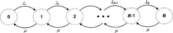
Figure 3 State transition diagram for a SSM/M/1/B self-similar queuing system.

$$\begin{array}{l}{\lambda }_j=\lambda (i,n,H);j=1,2,\dots ,B\hfill \\ {\lambda }_j=0:j\ge B+1\hfill \\ {\mu }_j=\mu ;j=1,2,\dots ,B+1\hfill \end{array}(44)$$

This system is stable with a throughput $\rho =\frac{\lambda (i,n,H)}{\mu }<1$. Let us consider two separated cases: ρ =1, and ρ ≠ 1. For j = 0,1,2,…, B the distribution of the number of flows in the system is P_j = ρ ^j P₀, which is determined according to

$$\begin{array}{l}{P}_J=\frac{{\rho }^j(1-\rho )}{1-{\rho }^{B+1}};\rho \ne 1\hfill \\ P_j=\frac{1}{B+1};\rho =1\hfill \end{array}(45)$$

Therefore, the rate at which the flows are blocked and lost is $\lambda P_B.$ The self-similar queuing process is described with the steady-state simulation procedure [16], presented in Figure 4.

The self-similar traffic can be generated and the sequence of arrivals is obtained. The fixed length of self-similar traffic is extracted by fixing the number of observations. As the service process is Markovian, the sequence of departures has exponential distribution, generated with an inverse transform generator [14].

The next step is the calculation of the buffer size. If the service size is greater than the size of arrivals, then the buffer size B = 0, as it is impossible to have a negative buffer size. In cases when the buffer size is greater than the overflow L, i.e. B > L, the traffic is lost, therefore we have made an assumption that B = L.

The simulation is performed with splitting of the sample path [15], using a variant based on the RESTART method [7], where any chain is split by a fixed factor when it hits a level upward, and one of the copies is tagged as the original for that simulation level. When any of those copies hits that same level downward, if the copy is the original it just continues its path, otherwise it is killed immediately. This rule applies recursively, and the method is implemented in a depth-first fashion, as follows: whenever there is a split, all the non-original copies are simulated completely, one after the other; then the simulation continues for the original chain [20].

The reason for eliminating most of the paths that go downward is to reduce the work. Therefore, the buffer size calculations being made for all sequences provide the opportunity to estimate the overflow probability using the steady-state simulation based on the RESTART method with the limited relative error (LRE) algorithm.

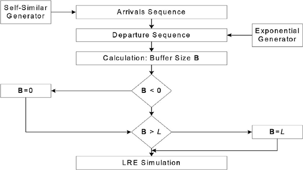
Figure 4 Steady-state simulation of self-similar queuing system.

3.3 RESTART Method with Limited Relative Error Algorithm and Simulation Results

The limited relative error algorithm helps to determine the complementary cumulative function of arrivals at single server buffer queues with Markov processes. In order to describe the LRE princilpes for steady-state simulation in Discrete-Time Markov Chains (DTMC), let us consider a homogeneous two-node Markov chain, which is extended to regular DTMC, consisting of (k + 1) nodes with states, respectively S₀, S₁,..,., S_k, as shown in Figure 5.

We obtain the random generated sequence x₁, x₂,…, x_t, x_t+1… for x = 0, l,…, k, for which a transition for state S_j at the time t exists, e.g. x_t = j and there are no constraints to the parameters of the transition probabilities:

$$P_{ij}=P(j|i);(i,j)=0,1,\dots ,k;{\displaystyle \sum _{j=1}^k{p}_{ij}}=1(46)$$

There are no absorbing states S_i, at p_ii = 1 for all stationary probabilities P_jj =0,1,…,k, which satisfy the constraint condition:

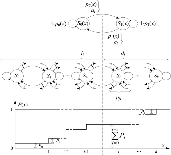
Figure 5 Cumulative function F(x) for (k + 1)-node Markov chain.

$$0\le P_j<1;{\displaystyle \sum _{j=0}^k{P}_j}=1(47)$$

The cumulative distribution F(x) can be presented as:

$$\begin{array}{l}\begin{array}{l}F(x)=F_i;(i-1)\le x<i;i=1,2,\dots ,k+1;\hfill \\ F_i={\displaystyle \sum _{j = 0}^{i-1}{P}_j};F_0=0;F_{k+1}=1;\hfill \end{array}\}\hfill \end{array}(48)$$

In order to simulate the (k+1) nodes of Markov chain, the complementary cumulative distribution G(x) = 1 –F(x) that is more significant, can be determined along with the local correlation coefficient ρ(x) through the limited relative error approach.

After having the homogeneous two-node Markov chain defined as shown in Figure 3, with changing the states n times, an estimation of the local correlation coefficient $\widehat{\rho }(x)$ can be obtained, which connects the number of transitions through a dividing line a_i ≈ c_i, with the total number of observed events l_i = n–d, (β = 0,1,…i - 1,) at left side, and d_i, at right side(β = i,i + 2,…, k).

The value of simulated complementary cumulative distribution ${\widehat{G}}_i$ can be defined directly by using relative frequency d_i/n, if there is enough number of samples:

$$n\ge {10}^3;(l_i,d_i\ge {10}^2);(a_i,c_i,l_i-a_i,d_i-c_i)\ge 10(49)$$

The posterior equations can be used for the complementary function $\widehat{G}(x)$, the average number of generated values of $\widehat{\beta }$, the local correlation coefficient $\widehat{\rho }(x)$, the correlation coefficient Cor[x] and the relative error RE[x]:

$$\begin{array}{l}\widehat{G}(x)={\widehat{G}}_i=d_i/n\widehat{\beta }=\frac{1}{n}{\displaystyle \sum _{i = 1}^k{d}_i}\hfill \\ \widehat{\rho }(x)={\widehat{\rho }}_i=1-\frac{c_i/d_i}{1-d_i/n}i-1\le x<i\hfill \\ i=1,\dots ,k\hfill \end{array}(50)$$

$$\begin{array}{l}\text{Cor}[x]={\text{Cor}}_i=(1+{\widehat{\rho }}_i)(1-{\widehat{\rho }}_i)\text{RE}{[x]}^2={\text{RE}}_i=\frac{1-d_i/n}{d}·{\text{Cor}}_i\hfill \end{array}$$

The main advantage of this approach is that the relationships between transitions c_i are obtained with routine statistical calculations. The necessary total number of simulation trails n is determined with the maximal relative error RE_max[x]² and with the less value of the function G(x), presented as $G_{\min }={\widehat{G}}_k$ in approximation equation:

$$\begin{array}{l}n=\frac{(1-G_{\min })}{G_{\min }.{\text{RE}}_{\max }{[x]}^2}\approx \frac{{\text{Cor}}_k}{{\widehat{G}}_k.{\text{RE}}_{\max }{[x]}^2};\hfill \\ {\text{Cor}}_k=\frac{1+{\widehat{\rho }}_k}{1-{\widehat{\rho }}_k}\hfill \end{array}(51)$$

This method can be described with a standard version of limited relative error algorithm for random discrete sequences of buffer arrivals. It consists of the following three steps provided below.

Algorithm 3 Restart with Limited Relative Error Simulation Method

$$d_i={\displaystyle \sum _{j=1}^k{h}_j}\text{for}i=0,1,\dots ,k\text{where}{d}_o=n(52)$$

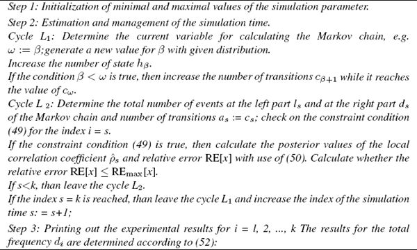
The values of the complementary function ${\widehat{G}}_i$, the local correlation coefficient ${\widehat{\rho }}_s$ and the relative error RE[x] are calculated as given in (50).

As an example, the overflow probability of an SSM/M/1/B self-similar queuing system has been simulated with different characteristics of long-range dependent self-similar arrival processes. In order to demonstrate the effects of self-similarity on the buffer overflow probability, the obtained experimental results were compared with the complementary cumulative distribution in the traditional single server finite buffer queue M/M/1/B. The obtained results in a logarithmic scale are given in Figure 6.

In order to get representative and steady results the sequences of 10000 observations were used. With the suggested LRE algorithm the values of complementary cumulative function G(x) for different buffer sizes were calculated. The calculations were provided with the step m = 4. One can see in Figure 6 that the increasing Hurst parameter has led to an insignificant decrease in the overflow probability.

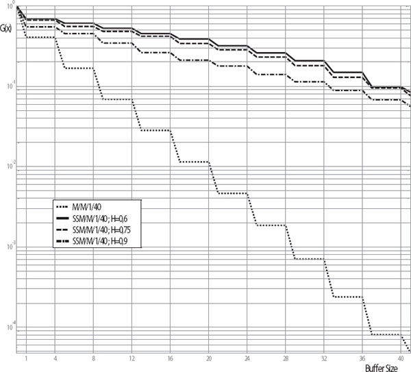
Figure 6 Buffer overflow probability (L = 41) in SSM/M/1/40 self-similar queuing system.

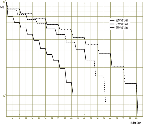
Figure 7 Buffer overflow probability in SSM/M/1/B self-similar queuing system with different buffer sizes.

For example, for the value of Hurst parameter H = 0.6 the overflow probability was G(L) = 1.045*10^-1, and for H = 0.9 it was G(L) = 5.6*10^-2. On the other hand, the overflow probability of self-similar queuing system has increased significantly in comparison with the theoretical M/M/1/B self-similar queuing system, for which G(L) = 4.79*10^-5.

After that, the simulation was repeated for SSM/M/1/B self-similar queuing system by using long-range dependent self-similar arrival process with H = 0.6 and different buffer sizes. The obtained results for buffer size B = 40, B = 60 and B = 80 are shown in Figure 7. One can see that since the buffer size was increased twice, the overflow probability has been changed simply by about two orders of magnitude – from 1.045*10^-1 to 6.4*10^-3.

Finally, it was confirmed that in order to design a single server finite buffer model with long-range dependent self-similar arrival processes, the buffer size has to be increased many times in order to decrease the overflow probability.

4 Conclusions

The paper recommends new methods to estimate effectively the probability of buffer overflow in high-speed communication networks. The frequency of buffer overflow in queuing systems is very small; therefore the overflow can be defined as rare event and estimated using rare event simulation with Markov chains.

Initially, two-node queuing systems have been considered in this paper; and an event of buffer overflow at the second node was studied. Two efficient rare event simulation algorithms, based on the Importance sampling and Cross-entropy methods, have been developed and applied to accelerate the buffer overflow simulation with Markov chain modeling. Simulation results were shown and analyzed.

Then, steady-state simulations of self-similar queuing systems have been conducted using the RESTART method with Limited Relative Error algorithm to estimate effectively the probability of buffer overflow. The models of SSM/M/1/40 self-similar queuing system have been applied with different parameters of arrival processes and different buffer sizes. Simulations results were shown and analyzed.

The resulting recommended methods to estimate effectively the probability of buffer overflow are appropriate and particularly efficient being used for performance evaluation in high-speed communication networks, while higher performance networks must be described by lesser buffer overflow probabilities.

Acknowledgements

The author would like to thank her colleagues Michael R. Bartolacci from Penn State University – Berks, USA and Cees J.M. Lanting from CSEM, Switzerland for their time, thoughtful insights and review during the preparation of this paper.

References

[1] Bobbio, A., Horváth, A., Scarpa, M., Telek, M. “Acyclic discrete phase type distributions: Properties and a parameter estimation algorithm.” Performance Evaluation, 54(1), 1–32, 2003.

[2] Bolch, G., Greiner, S., Meer, H, Trivedi, K. Queueing Networks and Markov Chains: Modeling and Performance Evaluation with Computer Science Applications, NY: John Wiley & Sons, 1998.

[3] Bueno, D. R., Srinivasan, R., Nicola, V., van Etten, W., Tattje, H. “Adaptive Importance Sampling for Performance Evaluation and Parameter Optimization of Communication Systems.” IEEE Transactions on Communications, 48(4), 557–565, 2000.

[4] Bucklew, J. “An Introduction to Rare Event Simulation.” Springer Series in Statistics, XI, Berlin: Springer-Verlag, 2004.

[5] C´erou, F., LeGland F., Del Moral P., and Lezaud P. “Limit theorems for the multilevel splitting algorithm in the simulation of rare events”. Proceedings of the 2005 Winter Simulation Conference, San Diego, USA, 682–691, 2005.

[6] De Boer, P., Kroese, D., Rubinstein, R. “Estimating buffer overflows in three stages using cross-entropy.” Proceedings of the 2002 Winter Simulation Conference, San Diego, USA, 301–309, 2002.

[7] Georg, C., Schreiber, F. “The RESTART/LRE method for rare event simulation”, Proceedings of the Winter Simulation Conference, Coronado, CA, USA, 390–397, 1996.

[8] Giambene, G. Queueing Theory and Telecommunications: Networks and Applications. NY: Springer, 2005.

[9] Heidelberger, P. “Fast Simulation for Rare Event in Queueing and Reliability Models.” ACM Transactions of Modeling and Computer Simulation, 5 (1), 43–85, 1995.

[10] Kalashnikov, V. Geometric Sums: Bounds for Rare Events with Applications: Risk Analysis, Reliability, Queueing. Berlin: Kluwer Academic Publishers, 1997.

[11] Keith, J., Kroese, D.P. “SABRES: Sequence Alignment by Rare Event Simulation.” Proceedings of the 2002 Winter Simulation Conference, San Diego, USA, 320–327, 2002.

[12] Kroese, D., Nicola, V.F. “Efficient Simulation of a Tandem Jackson Network.” Proceedings of the Second International Workshop on Rare Event Simulation RESIM'99, 197–211, 1999.

[13] Lokshina, I. “Study on Estimating Probability of Buffer Overflow in HighSpeed Communication Networks.” Proceedings of the 2014 Networking and Electronic Commerce Conference (NAEC 2014, Trieste, Italy, 306–321, 2014.

[14] Lokshina, I. “Study about Effects of Self-similar IP Network Traffic on Queuing and Network Performance.” Int. J. Mobile Network Design and Innovation, 4(2), 76–90, 2012.

[15] Lokshina, I., Bartolacci M. “Accelerated Rare Event Simulation with Markov Chain Modelling in Wireless Communication Networks.” Int. J. Mobile Network Design and Innovation, 4(4), 185–191, 2012.

[16] Radev, D., Lokshina, I. “Performance Analysis of Mobile Communication Networks with Clustering and Neural Modelling”. Int. J. Mobile Network Design and Innovation, 1(3/4), 188–196, 2006-a.

[17] Radev, D., Lokshina, I. “Rare Event Simulation with Tandem Jackson Networks.” Proceedings of the Fourteen International Conference on Telecommunication Systems: Modeling and Analysis – ICTSM 2006, Penn State Berks, Reading, PA, USA, 262–270, 2006-b.

[18] Radev, D., Lokshina, I. “Advanced Models and Algorithms for Self-Similar Network Traffic Simulation and Performance Analysis”, Journal of Electrical Engineering, Vol. 61(6), 341–349, 2010.

[19] Rubino G, Tuffin B. Rare Event Simulation using Monte Carlo Methods, UK: John Wiley & Sons, 2009.

[20] Villen-Altamirano, M., Villen-Altamirano, J. “On the efficiency of RESTART for multidimensional systems.” ACM Transactions on Modeling and Computer Simulation, 16 (3), 251–279, 2006.

Biography

I. Lokshina, PhD is Professor of Management Information Systems and chair of Management, Marketing and Information Systems Department at SUNY Oneonta. Her positions included Senior Scientific Researcher at the Moscow Central Research Institute of Complex Automation and Associate Professor of Automated Control Systems at Moscow State Mining University. Her main research interests are complex system modeling (communications networks and queuing systems) and artificial intelligence (fuzzy systems and neural networks).

Journal of Cyber Security, Vol. 3, 399–426.
doi: 10.13052/jcsm2245-1439.343
© 2015 River Publishers. All rights reserved.

Abstract

Keywords

1 Introduction

2 Estimating Probability of Buffer Overflow in Continuous Time Queueing Systems

2.1 Rare Event Simulation with Markov Chain Modeling

2.2 Exponential Change of Measure

2.3 Importance Sampling Algorithm and Simulation Results

2.4 Cross-Entropy Algorithm and Simulation Results

3 Estimating Probability of Buffer Overflow in Self-Similar Queuing Systems

3.1 Long-Range Dependent Self-Similar Processes

3.2 Steady-State Simulation with SSM/M/1/B Modeling

3.3 RESTART Method with Limited Relative Error Algorithm and Simulation Results

4 Conclusions

Acknowledgements

References

Biography