Mobility Improvement by Optimizing Channel Model Coverage Through Fine Tuning
Akansha Gupta*, Kamal Ghanshala and R. C. Joshi
Department of Computer Science and Engineering, Graphic Era Deemed to be University, Dehradun, India
E-mail: akanksha3000@gmail.com; kamalghanshala@gmail.com; chancellor.geu@gmail.com
*Corresponding Author
Received 09 January 2021; Accepted 20 February 2021; Publication 25 May 2021
Abstract
Empirical channel models were always an important tool for proper wireless network planning. These models consider the properties of electromagnetic waves and terrain conditions. The efficiency and accuracy of these Empirical models suffer when they are used for an area other than where they have been designed. So tuning of these models is required for proper and accurate prediction of coverage and it is done by taking the correction factor into account. Comparison of four Empirical models i.e, the Lee, the ECC-33 model, the WI model, the Ericsson model, the COST 231, and SUI is done with Measured path loss, and the best model with minimum error is then selected for tuning. Field data of LTE network at 2300 MHz is collected at two sites of Uttarakhand-India. It is analysed that the Ericsson model shows minimum RMSE, Standard Deviation, and Mean error as compared to measured path loss, followed by the Okumura model. The Ericsson model is then tuned to further reduce the error. Validation of the tuned model is done at Haridwar.
Keywords: Tuning, mobility, VHF, pathloss models, RMSE, LTE.
1 Introduction
Over the past few years, there is an exponential rise in wireless applications e.g., augmented reality, IoT, 5G, healthcare, agriculture, etc. due to which there is a rise in the optimization of coverage of BTS [1–3]. To locate the correct geographical location of a Base Station Transmitter in an outdoor wireless network, path loss prediction is essential for the interest of researchers. Propagation of electromagnetic waves between Tx and Rx exhibits multiple reflections, deep fading, shadowing, etc. Empirical path loss models were used to calculate signal loss and coverage prediction. In recent survey reports of the Telecom Regulatory Authority of India (TRAI) and research survey on cellular mobile service, it is identified that call drop is among one of the major issues which result in deterioration of Quality of Service (QoS) of a wireless network [4]. Quality of Service of a wireless network depends on 4 major parameters:
• Accessibility
• Connection setup
• Connection continuation
• Routing
Connection maintenance is monitored through three factors:
• Call drop ratio
• Worst affected call
• Connection with good voice quality
As indicated by TRAI report higher call drop ratio depends upon the Radio Frequency (RF) related issues i.e. 50% of call drop occurs due to propagation factors such as reflection, multipath fading, diffraction, and shadowing of signal [5–8]. Table 1 shows different causes of call drop.
Table 1 Causes of call drop
| Call Drop Cause | Occurrence |
| Propagation Loss | 51.4% |
| Unpredictable user requirements | 36.9% |
| Unusual network reaction | 7.6% |
| Miscellaneous | 4.1% |
1.1 Need for Tuning
Empirical models suffer in their efficiencies when they were used in an environment other than where they have been designed, so they need to be tuned according to new terrain. Tuning is done by adding a correction factor to the best fit path loss model in new terrain [9–13].
1.2 Spline Interpolation
Spline Interpolation is a continuous second derivative mathematical equation that maps complete data onto a smooth curve. According to the spline theory for boundary condition of data points, n equations can be fit over n intervals. Mathematically, this method calculates the missed data points in the analysis of measured data. Therefore, spline Interpolation determines in-between missing point values to compute the accurate performance of empirical models. The signal strength has been measured around selected BTS but due to the limitations of terrain conditions like mountain, dense forest, the sharp valley it is not possible to collect field data at every possible distance. Tuning using spline interpolation has been used to find out path loss at such locations where it is difficult to reach with test equipment and not possible to collect field data. Here we have compared Empirical path loss models with measured path loss and analyzed missed out path loss using tuning and spline interpolation [14–16].
1.3 Contribution
The main contribution of this paper is to provide an exact solution for optimized coverage for fringe areas like Uttarakhand-India.
1. Comparison and selection of the best empirical model with minimum Root Mean Square Error (RMSE), Standard Deviation (SD), and Mean Absolute Error (MAE) w.r.t measured path loss.
2. Tuning of the best fit model by incorporating correction factors according to local terrain conditions.
3. Validation of the tuned model is done for similar fringe conditions.
We briefly describe the content in the following sections of the paper. In Sections 2 and 3 a literature review and an outline of Outdoor Propagation models is given respectively. In Section 4 we describe measurement setup with data collection methodology. Finally, in Sections 5 and 6, we report experimental results, discussions, conclusions, and future scope which clearly show the usefulness of the tuning and spline interpolation approach in predicting and maximizing wireless signal coverage.
2 Literature Review of Related Work and Contextualization
Researchers have used the Friis Free Space Path Loss (FSPL) model to predict signal coverage in an uninterrupted LoS path. In Tokyo, Okumura presented a model that predicts received signal coverage at 2 GHz frequency over the collected data [16, 17]. HATA additionally extended Okumura Model by incorporating graphical information along with fading effects in a mathematical expression [16]. HATA model when used in rural and sub-urban areas of Malaysia, Roslee et al. incorporated a correction factor to give a better prediction [18]. In Mosul city, Iraq data collection was conducted in a suburban and urban environment at 1800 and 900 MHz frequency whose analysis showed that tuning factor is required to predict signal strength over an uneven geographical area by using the models Walfisch-Ikegami (WI), Lee, Cost-231, International Telecommunication Union (ITU-R), Ericsson, and Stanford University Interim (SUI) [19, 20]. The Model reflecting the minimum value of RMSE between a predicted and a measured value of the RMSE is selected as the best. Also, the author recommended a signal mapping model for maximum coverage by applying an S-shaped sigmoid function on the measured data with the help of neural networks [21]. A wireless coverage predictive model is built for radio access networks (RAN) by employing a crowd-sourced examination of the Long-Term Evaluation (LTE) network. Machine learning methods like the Gaussian Process, Random Forest, and Exponential smoothening of time series are applied and investigated over data gathered from conducting a thorough drive test for signal coverage mapping which provides better coverage [22, 23]. It simultaneously provides better user quality as well as less operational cost. Fixed Rank Kriging (FRK) algorithm provides an efficient prediction of signal strength of the places which are not accessible for field measurement [23, 24]. Through spatial interpolation of geographically co-located measurements, a coverage map has been framed using FRK. Machine-learning models for estimating path loss of different terrain and vegetation surroundings have been explored by many authors [24–28]. For the investigation, four machine learning algorithms were considered. Random Forest demonstrates minimum error value with better accuracy. A 37% reduction in average prediction error has been achieved through machine learning models. Extensive field measurements have been conducted by several researchers to collect a Received Signal Strength Indicator (RSSI) to provide optimized coverage and angular power. Particle Swarm Optimization was used to tune propagation models which were then compared with the Okumura HATA model and results demonstrated that the tuned propagation model performs better [12, 40–42].
3 Outdoor Propagations
The outdoor propagation model has been broadly classified into 3 broad categories Figure 1:
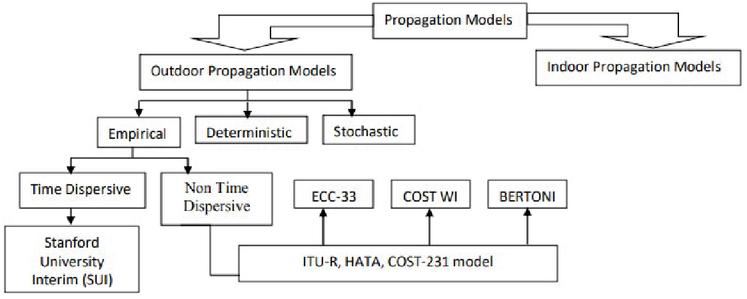
Figure 1 Classification of outdoor empirical models.
3.1 Empirical Propagation Models
These models make use of measured and observed data only. It is further classified as:
(a) Time Dispersive (SUI)
(b) Non-Time Dispersive (HATA, COST-231, ITU-R)
3.2 Deterministic Propagation Models
In Deterministic propagation models received signal strength at specific terrain is calculated by using laws of electromagnetic wave propagation. 3D design of a building or specific terrain like foliage is constructed from the dataset thereafter fundamental environmental effects like diffraction, reflection and scattering will be analysed using ray-tracing techniques.
3.3 Stochastic Models
These models were designed to analyse changes in the radio wave’s behaviour due to random factors.
This paper represents the critical analysis of empirical propagation models and a relative comparison is made between measured and predicted path loss value.
Empirical Models selected for the current analysis are:
(1) COST-231 Model
(2) SUI Model
(3) Ericsson Model
(4) ECC-33 Model
(5) Walfisch Ikegami Model
(6) Lee Model
(1) COST-231 Model
HATA model is designed with a limitation of having upper frequency up to 1500 MHz however systems like GSM which uses 1800 MHz cannot use the HATA model due to 1500 MHz frequency limitation [29]. Extension of frequency from 1500 MHz to 2000 MHz had been achieved using COST-231 median path loss model:
| (1) |
where
is frequency in MHz
is distance between and (in km)
and is effective height of and antenna (in meters)
is 0 dB for suburban and rural terrain
3 dB for urban terrain
for small to medium city is expressed as:
for large city in dB
Range of parameters for COST-231 model
(2) Stanford University Interim (SUI Model)
The frequency range of the HATA model is extended from 1800 MHz to 11 GHz by IEEE 802.16 wireless group by proposing the SUI model [12, 30]. This model incorporates correction factors due to terrain and foliage based distribution. SUI model is expressed as:
| (2) |
where
distance between Tx and Rx (in km)
wavelength
, , Correction factor for frequency, receiving antenna height and shadowing effect
GHz
Factor ‘e’ considers shadowing due to foliage and similar terrain condition, it is basically a log-normal distribution and it’s whose values vary between 8.2 to 10.6 dB.
(3) Ericsson Model
Ericsson proposed a model that can change the parameters according to the propagation environment [31–32].
It is expressed as:
| (3) |
where,
(4) ECC-33
ECC-33 is proposed by Electronic Communication Committee (ECC) and is a modified Okumura model extending its range up to GHz.
| (4) |
where,
: Attenuation (dB)
: Median path loss
: Transmitting antenna gain
: Receiving antenna gain
(5) Walfisch Ikegami Model
It is an extension of the Walfisch and Bertoni model which calculates the diffraction effect of rooftop and building heights at streets. It considered the effect of reflection and scattering between high-rise civil structures in urban areas under a line of sight (LOS) and non-line of sight (NLOS) conditions. It works in the frequency range of 800 MHz to 2 GHz and BTS heights up to 45 m.
(6) Lee Model
W.C.Y. Lee in the year 1982 proposed the Lee model which is divided into two parts
1. Area to Area model: It predicts path loss over flat terrain and fails to predict path loss due to hilly terrain.
2. Point to Point Model: This model is developed from Area to Area model and consider LOS and NLOS condition. For LOS condition, influence of reflected waves is studied and for NLOS condition diffracted waves due to obstruction is modeled using knife edge effect.
Lee Area to Area model is expressed as:
| (5) |
where
is signal power (in watts) at receiver
is signal power (at the point of interaction) at a distance of from the transmitter
is signal frequency
is reference signal frequency
is the adjustment factor for the antenna height transmitter power and antenna gains
is the path loss slope
4 Experimental Setup and Data Collection
Measurement campaign for current research has been carried out at three different terrains of Uttarakhand, India and having coordinates which lies within 29.9457N longitude, and 78.1642E latitude. Uttarakhand is situated at the foothills of the Himalayan region and having a fringe terrain covering trees, mountains, forest, rain, snow, fog, and free space. Due to the holy river Ganga, this region remained covered with fog during the months of December-January. Uttarakhand is chosen to analyze the combined effect of the forest, mountains, and mixed terrain canopies. Many researchers have applied a similar approach of path loss prediction in their terrain i.e Nigeria [33–36], Malaysia [19], Jinan [37], Africa [38], United Kingdom [30] for tuning and path loss prediction as well as to analyze the effect of terrain on signal propagation comprehensive field measurements was carried out during 2019–20. Sites Dehradun, Haridwar, and Rishikesh were identified to observe variation in terrain and climatic condition on signal propagation.
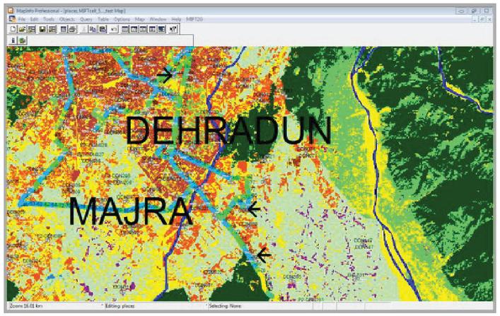
Figure 2 The 16 clusters (4 BTS each) at, Uttarakhand-India.
An area of about 25 km was covered at each site by forming 16 clusters (4 BTS each) as shown in Figure 2. The location of BTS is selected to cover the maximum effect of terrain conditions on signal propagation. Field drive testing has been carried out to calculate the average value of the Received Signal Strength Indicator (RSSI). The 360-degree region around BTS is divided into 3 sectors alpha, beta, and gamma separated by 120 degrees apart as shown in Figure 3 and threshold values of network coverage in these sectors were tabulated in Table 2.

Figure 3 Sectoral alignment of 3 sectors around BTS.
Table 2 Threshold value in 3 sectors
| Network Threshold | Value |
| Coverage Objective RSRP (dBm) | 102.6 |
| Coverage Overshooting Radius (m) | 4005 |
| Coverage Overshooting RSRP (dBm) | 90.0 |
| Coverage Overshooting Percentile (%) | 8 |
| Coverage Swap Percentile (%) | 46 |
Navigation tools like CATIA, XCAL, and TEMS were used to collect RSSI around selected BTS using drive vehicle, laptop, Garmin global position system (GPS), sockets, test cables, Sony mobile handset equipped with TEMS navigation software, MapInfo or Deskcat, and drive test route [28, 35, 39]. GPS was mounted on the vehicle and uses the Sony Ericson mobile handset.RSS measurements were recorded at each test point around the selected base stations (BS) covering all roads, forest, mountain, and populated areas as shown in Figure 4.
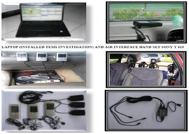
Figure 4 3D Drive test tool.
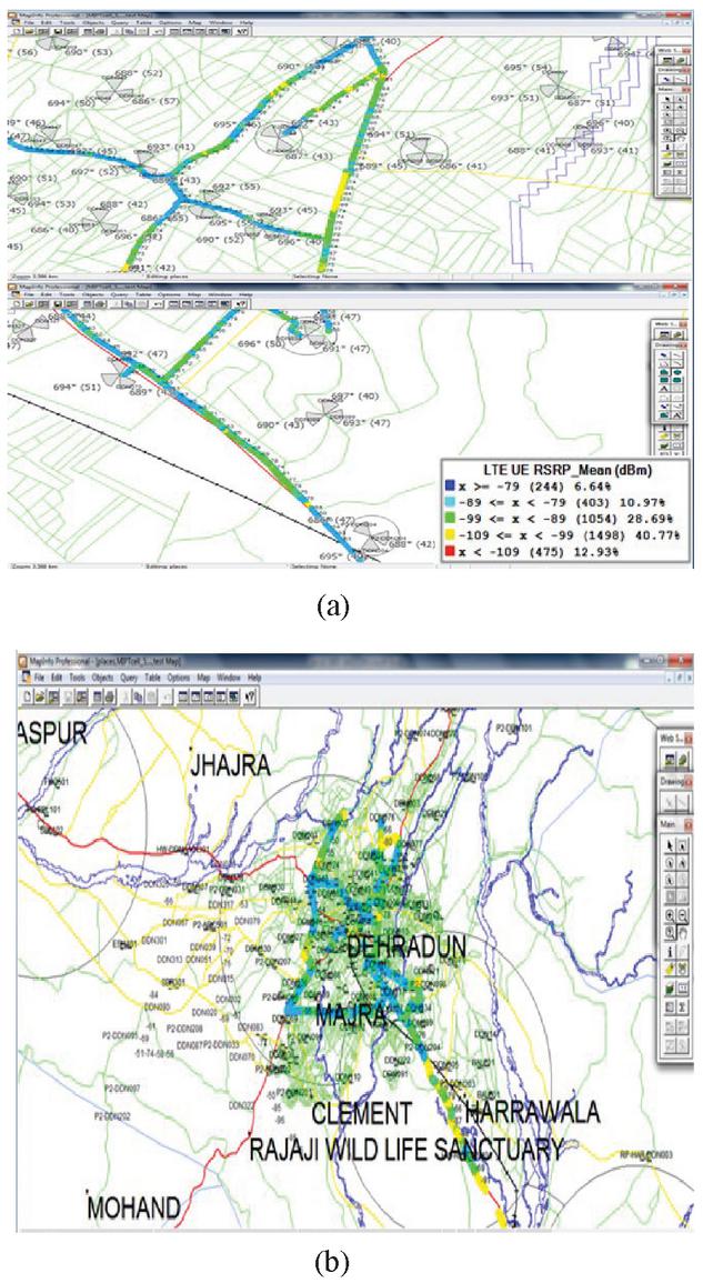
Figure 5 Drive test route. BTS is identified by 3-letter codename.
Drive test route is shown in Figure 5 where RSSI is indicated by the color bar, good signal strength is indicated by the blue color bar having a value less than 79 dBm and red color bar is having worst signal strength greater than 109, the yellow color bar indicates field strength ranging from 109 to 99.

Figure 6 Signal coverage around drive test cell boundary.
Table 3 Parameters of outdoor network
| Parameters | Value |
| Cluster Sectors | I-UW-GGLT-ENB-9003 |
| Band | 1800 |
| Antenna Longitude | 80.06384556 |
| Antenna Latitude | 29.57544 |
| Antenna Height (m) | 35 |
| Antenna Azimuth | 8 |
| Antenna Tilt Electrical, Mechanical | 7, 5 |
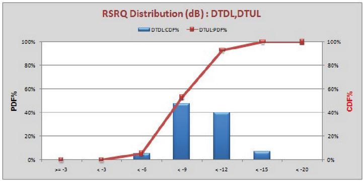
Figure 7 RSRQ Distribution (dBm) of DTDL, DTUL.
Figure 6 illustrates the Signal coverage around drive test cell boundary.
Table 3 tabulates the parameters of outdoor network along with their values. Received Signal Received Power Quality (RSRQ) is the power of the LTE reference signals which is distributed over the full bandwidth. The range of RSRQ varies between 140 dBm to 44 dBm along with a resolution of 1 dB. Figure 7 represents the distribution of collected RSRQ ranging from 79 to 109 thus lies within the RSRQ range.
5 Experimental Results and Discussions
Analysis Comparison of Selected Empirical Propagation Models with Field Measured Path Loss
Propagation models were analyzed using the data collected from field for optimized coverage prediction at selected sites. Firstly Path loss is calculated at Dehradun from the measured data at a regular interval of 100 m ranging from 100 m to 2000 m and it is tabulated in Table 4.
Table 4 Measured path loss at distance of 100 m at Dehradun
| Distance | Pathloss | Distance | Pathloss |
| 100 | 123 | 1100 | 155 |
| 200 | 124 | 1200 | 159 |
| 300 | 140 | 1300 | 158 |
| 400 | 134 | 1400 | 159 |
| 500 | 138 | 1500 | 155 |
| 800 | 152 | 1800 | 164 |
| 900 | 147 | 1900 | 165 |
| 1000 | 152 | 2000 | 168 |
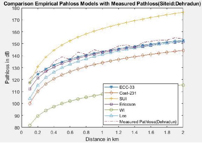
Figure 8 Analysis of Empirical path loss prediction models with measured path loss at Dehradun.
Selected propagation models are compared with the measured path loss and its analysis is shown in Figure 8. SUI path loss model shows maximum RMSE while ECC-33 fits nearest to measured data followed by the Ericsson model.
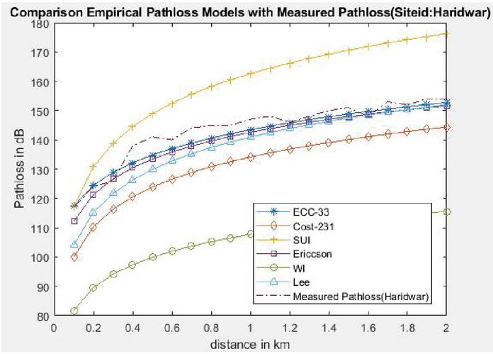
Figure 9 Analysis of Empirical path loss prediction models with measured path loss at Haridwar.
Analysis of empirical path loss prediction models with measured path loss at Haridwar and Rishikesh is shown in Figures 8 and 9 and it is analyzed ECC-33 and Ericsson model lies nearest to measured path loss.
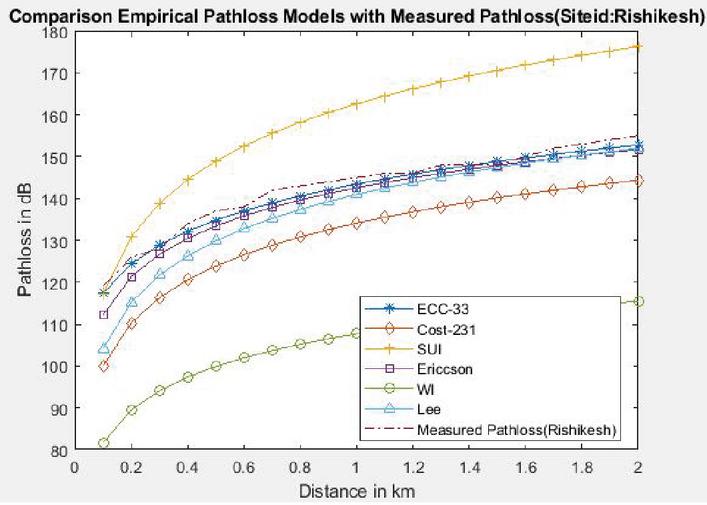
Figure 10 Analysis of Empirical path loss models with measured path loss at Rishikesh.
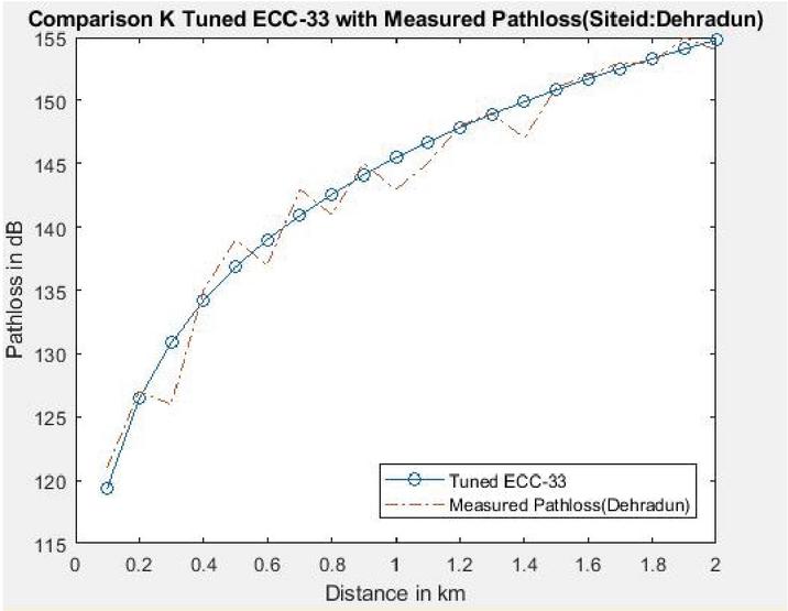
Figure 11 Comparison of K tuned ECC-33 with measured path loss at Dehradun.
Observations from Figures 6–10 represents that the ECC-33 model predicts path loss nearest to the path loss value obtained from the collected data. Prediction accuracy of the ECC-33 model is highest followed by Ericsson and Lee model. The predicted value of the ECC-33 model is nearly equal to the value of path loss calculated from measured data. Propagation models show a deviation in the result when they are used in an environment other than for which they have been designed. Therefore, for improving their prediction efficiency tuning factor needs to be added to the original ECC-33 model.
Tuned ECC-33 model
ECC-33 model is applied in a region of Uttarakhand which is other than where it was designed originally, so for optimum performance it is needed to tune the ECC-33 model for the Uttarakhand region. Thus a correction factor is added based on the Root Mean Square Error (RMSE). The RMSE for Dehradun is 2.6957. So it is proposed that the tuned ECC-33 model can be expressed as:
Path Loss value of tuned ECC-33 model = Path loss of original ECC-33 Model RMSE value at Dehradun
| Tuned PL ECC-33 Model PL ECC-33 2.6957 |
Analysis of Figures 10 and 11 shows the measured path loss, path loss predicted by the ECC-33 model, and tuned ECC-33 model. Table V represents the RMSE value of selected models along with tuned ECC-33 Model. RMSE value of the tuned ECC-33 Model is 1.5440 which is quite acceptable. It can be concluded from Figure 11, that the tuned ECC-33 Model provides improved performance as compared to the original ECC-33 Model for the Dehradun fringe region of Uttarakhand. The tuned ECC-33 model provides better results when applied to another region of Uttarakhand similar to Dehradun.
To validate the tuned ECC-33 model, it is applied at Rishikesh where environmental conditions are similar to Dehradun. A drive test is conducted for a distance ranging from 100 m to 2000 m and field data is collected between the transmitter-receiver pair. Figures 12 and 13 shows the error value between empirical and tuned model at a regular interval of distance.
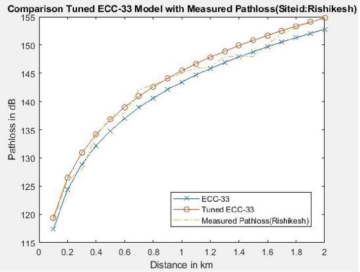
Figure 12 Comparison between tuned ECC-33 model with Empirical path loss models at Rishikesh.
Table 5 Mean and standard deviation of propagation models
| Model | Mean | Standard Deviation |
| ECC-33 | 141.5094 | 9.8184 |
| SUI | 158.9304 | 16.033 |
| COST 231 | 131.3651 | 12.025 |
| Ericsson | 140.1028 | 10.717 |
| Walfisch-Ikegami (WI) | 137.9656 | 9.1769 |
| Lee | 105.6074 | 12.988 |
The mean value and standard deviation of propagation models and measured path loss are tabulated in Table 5.
Table 6 RMSE error of empirical path loss models
| Model | RMSE |
| ECC-33 | 2.6957 |
| SUI | 299.09 |
| COST 231 | 136.92 |
| Ericsson | 9.4172 |
| Tuned ECC-33 | 1.5440 |
| Walfisch-Ikegami (WI) | 1384.8 |
| Lee | 34.6531 |
Table 6 shows the RMSE error of empirical path loss models w.r.t measured path loss. ECC-33 model was observed to have a minimum RMSE of 2.6957.

Figure 13 Comparison of error between Empirical Path loss Models vs Measured Path loss at Dehradun.
Results of Figures 13 and 14 clearly show that the improved results are given by the tuned ECC-33 model at the Rishikesh region as compared to the basic ECC-33 path loss Model.
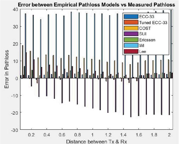
Figure 14 Comparison of error between Empirical Path loss Models vs Measured Path loss at Rishikesh.
6 Conclusion and Future Work
Empirical path loss models have been compared with measured path loss in the fringe areas of the Uttarakhand-India region. Individually propagation models have been analyzed for different topography and environmental conditions. These environmental variations have been studied at a given frequency range.ECC-33 has been analyzed with the COST-231 Model, SUI Model, Ericsson Model, ECC-33 Model, Walfisch Ikegami Model, and Lee model. Observations showed that for a Uttarakhand fringe region ECC-33 model predicts better results which are represented as Mean Absolute Error (MAE), Standard Deviation and Root Mean Square Error (RMSE) values. For increasing prediction accuracy of the ECC-33 model it is tuned according to the fringe environmental condition of Uttarakhand. Tuned ECC-33 reduces the RMSE by 1.1517. For validation tuned ECC-33 model was applied to Rishikesh i.e. a region similar to Dehradun where it again provides minimum RMSE. Researchers can design machine learning propagation model using current approach.
References
[1] T. S. Rappaport, S. Sun, M. Shafi, Investigation and comparison of 3GPP and NYUSIM channel models for 5G wireless communications, IEEE 86th Vehicular Technology Conference, VTC-Fall, 2017, September, pp. 1–5, doi: 10.1109/VTCFall.2017.8287877
[2] S. Sun, G. R. MacCartney, T. S. Rappaport, A novel millimeter-wave channel simulator and applications for 5G wireless communications, IEEE International Conference on Communications, 2017, May, pp. 1–7, doi: 10.1109/ICC.2017.7996792
[3] S. Salous, J. Lee, M.D. Kim, M. Sasaki, W. Yamada, X. Raimundo, A. A. Cheema, Radio propagation measurements and modeling for standardization of the site general path loss model, International Telecommunications Union recommendations for 5G wireless networks, In Radio Science Journal, (2020). Vol. 55, no. 1, Jan. 2020, doi: https://doi.org/10.1029/2019RS006924
[4] TRAI report “https://www.trai.gov.in/about-us/annual-reports”
[5] Z. Zhimeng, Z. Jianyao, Chao Li, Coverage Estimation in Outdoor Heterogeneous Propagation Environments, International Journal of Antennas and Propagation, Vol. 2019, pp. 1–10, doi: 10.1155/2019/3981678
[6] V. Kristem, S. Sangodoyin, C. U. Bas, 3D MIMO outdoor-to-indoor propagation channel measurement, IEEE Transactions on Wireless Communications, vol. 16, no. 7, pp. 4600–4613, 2017, doi: 10.1109/GLOCOM.2015.7417827
[7] E. T. Tchao, J. D. Gadze, J. O. Agyapong, Performance evaluation of a deployed 4G LTE network, International Journal of Advanced Computer Science and Applications, vol. 9, no. (3), pp. 165–178, April 2018, doi: 10.14569/IJACSA.2018.090325
[8] A. Neskovic, N. Neskovic, G. Paunovic, Modern approaches in modeling of mobile radio systems propagation environment, IEEE Communications Surveys & Tutorials, vol. 3(3), pp. 2–12, doi: 10.1109/COMST.2000.5340727
[9] I. Khan, T. C. Eng, S. A. Kamboh, (2012), Performance Analysis of Various Path Loss Models for Wireless Network in Different Environments, International Journal of Engineering and Advanced Technology (IJEAT) ISSN, 2249–8958.
[10] M. Ekpenyong, J. Isabona, E. Ekong, (2010), On Propagation Path Loss Models For 3-G Based Wireless Networks: A Comparative Analysis, Computer Science & Telecommunications, vol. 25(2).
[11] T. Sarka., K. Kyungjung, A. Medouri, Magdelena, S. Palma, A survey of various propagation models for mobile communications, IEEE Antenna Propagation Magazine, 2003;45(3):3–10. [Google Scholar]
[12] L. Boithias, 1987, Radio wave propagation, McGraw-Hill Inc. New York St. Louis an Francisca Montreal Toronto, pp. 10–100. [Google Scholar]
[13] S. Kale, A. N. Jadhav, (2013). An Empirically Based Path Loss Models for LTE Advanced Network and Modeling for 4G Wireless Systems at 2.4 GHz, 2.6 GHz, and 3.5 GHz, International Journal of Application or Innovation in Engineering & Management (IJAIEM), 2(9), 252–257.
[14] V. Gupta, S. Sharma, M.C. Bansal, Fringe area path loss correction factor for wireless communication, International Journal of Recent Trends in Engineering, vol. 1, no. 2, pp. 30–32, May 2009, ISSN (online): 2455–1457.
[15] M.S. Mollel, M. Kisangiri, Comparison of empirical propagation path loss models for mobile communication, Computer Engineering Intell. Syst. 2014;5:1–10. [Google Scholar]
[16] T. Okumura, E. Ohmori, K. Fukuda, Field strength and its variability in VHF and UHF land mobile service, review Electrical communication laboratory. 1968;16:824–870. [Google Scholar]
[17] M. Hata, Empirical formula for propagation loss in land mobile radio services, IEEE transactions on Vehicular Technology, 29(3), (1980), pp. 317–325, doi: 10.1109/T-VT.1980.23859
[18] M. B. Roslee, K. F. Kwan, (2010), Optimization of Hata propagation prediction model in suburban area in Malaysia,Progress in Electromagnetic Research, 13, pp. 91–106. doi: 10.2528/PIERC10011804
[19] S. A. Mawjoud, Path loss propagation model prediction for GSM network planning, International Journal of Computer Applications, 2013-December, vol. 84, no. 7, pp. 30–33, doi: 10.5120/14592-2830
[20] H. Hammouti, M. Ghogho, S. Ali, R. Zaidi, A Machine Learning Approach to Predicting Coverage in Random Wireless Networks, IEEE Globecom Workshops, pp. 1–6, 2018, doi: 10.1109/GCWkshps43968.2018.
[21] A. Ghasemi, Data-Driven Prediction of Cellular Networks Coverage: An Interpretable Machine-Learning Model, 2018, IEEE Global Conference on Signal and Information Processing (GlobalSIP), pp. 604–608, 2018, doi: 10.1109/GlobalSIP.2018.8646338.
[22] J. Riihijarvi, P. Mahonen, Machine Learning for Performance Prediction in Mobile Cellular Networks, IEEE Computational Intelligence Magazine, pp. 51–60, vol. 13, Issue:1, 2018, doi: 10.1109/MCI.2017.2773824
[23] H. Braham, S. B. Jemaa, G. Fort, E. Moulines, B. Sayrac, Fixed Rank Kriging for cellular coverage analysis, IEEE Transaction Vehicular. Technology, vol. 66, no. 5, pp. 4212–4222, May 2017. doi:10.1109/TVT.2016.2599842
[24] A. Gupta, S. C. Sharma, S. Vijay, V. Gupta, Secure path loss prediction using fuzzy logic approach, 2008, Fourth International Conference on Wireless Communication and Sensor Networks, Allahabad, India, Dec. 2008, doi: 10.1109/WCSN.2008.4772717.
[25] C. Oroza, Z. Zhang, T. Watteyne, S. D. Glaser, A Machine-Learning Based Connectivity Model for Complex Terrain Large-Scale Low-Power Wireless Deployments, IEEE Transactions on Cognitive Communications and Networking, vol. 3, no. 4, Dec. 2017. doi: 10.1109/TCCN.2017.2741468
[26] H. Wang, S. Xie, K. Li, M. Omair Ahmad, Big Data-Driven Cellular Information Detection and Coverage Identification, sensor journal, vol. 19, no. 4, pp. 937–942, 2019, doi: 10.3390/s19040937.
[27] D. Djomadji, E. Michel, T. Emmanue, New Propagation Model Optimization Approach based on Particles Swarm Optimization Algorithm, International Journal of Computer Applications, vol. 118, no. 10, pp. 39-47, 2015, doi: 10.5120/20785-3430.
[28] COST 231. COST 231 TD (90) 119 Rev. 2, The Hague, the Netherlands. 1991. Urban transmission loss models for mobile radio in the 900 and 1800 MHz bands (revision 2) [Google Scholar]
[29] V. S. Abhayawardhana, I. J. Wassell, D. Crosby, M. P. Sellars, M. G. Brown, (2005, May). Comparison of empirical propagation path loss models for fixed wireless access systems. In 2005 IEEE 61st Vehicular Technology Conference (Vol. 1, pp. 73–77). doi: 10.1109/VETECS.2005.1543252
[30] A. E. Ibhaze, A. L. Imoize, S. O. Ajose, S. N. John, Ndujiuba, C. U. Idachaba, (2017). An empirical propagation model for path loss prediction at 2100 MHz in a dense urban environment. Indian Journal of Science and Technology, 10(5), 1–9. doi: 10.17485/ijst/2017/v10i5/90654
[31] K. J. Parmar, D. V. D. Nimavat, 2015, Comparative Analysis of Path Loss Propagation Models in Radio Communication, International Journal of Innovative Research in Computer and Communication Engineering, vol. 3, pp. 840–844. doi: 10.1109/ICPECA47973.2019.8975464
[32] A. Akinbolati, M. O. Ajewole, Investigation of path loss and modeling for digital terrestrial television over Nigeria, International Journal Heliyon 2020 Jun, Vol. 6, no. 6, doi: 10.1016/j.heliyon.2020.e04101
[33] S. O. Ajose, A. L. Imoize, (2013). Propagation measurements and modeling at 1800 MHz in Lagos Nigeria. International Journal of Wireless and Mobile Computing, 6(2), 165–174. doi: 10.1504/IJWMC.2013.054042
[34] O. Shoewu, A. Adedipe, F. O. Edeko, 2011, CDMA network coverage optimization in South-Eastern Nigeria, American journal of scientific and industrial research. 2(3):346–351. doi: 10.5251/ajsir.2011.2.3. 346.351
[35] A. Akinbolati, O. Akinsanmi, K.R. Ekundayo, Signal strength variation and propagation profiles of UHF radio wave channel in Ondo state, Nigeria, International Journal of Wireless Microwave Technology. (IJWMT) 2016;6(4):12–27. [Google Scholar]
[36] J. Wu, D. Yuan, Propagation measurements and modeling in Jinan city, Ninth IEEE International Symposium on Personal, Indoor and Mobile Radio Communications (Cat. No. 98TH8361), (1998, September), vol. 3, pp. 1157–1160, doi: 10.1109/PIMRC.1998.731360
[37] A. Halifa, E. T. Tchao, J. J. Kponyo, (2017), Investigating the Best Radio Propagation Model for 4G-WiMAX Networks Deployment in 2530MHz Band in Sub-Saharan Africa, arXiv preprint arXiv:1711.08065.
[38] S. Pattanayak, A Genetically Trained Neural Network for Prediction of Path Loss in Outdoor Microcell, International Journal of Advanced Research in Engineering and Technology (IJARET), vol. 11, no. 4, pp. 346–351, 2020. doi: https://ssrn.com/abstract=3599786
[39] U. P. Nterhuber, S. S. Pfletschinger and M. Soliman, Jost, A survey of channel measurements and models for current and future railway communication systems, Mobile Information Systems, June 2016, vol. 11, no. 6, pp. 1–14, doi: 10.1155/2016/7308604
[40] R. Mardeni, L. Y. Pey, 2012, Path loss model optimization for urban outdoor coverage using Code Division Multiple Access (CDMA) system at 822MHZ, Modern Applied Science, vol. 6, pp. 28. http://connection.ebscohost.com/c/articles/7063899
[41] M. S. Mollel, M. Kisangiri 2014, Comparison of Empirical Propagation Path Loss Models for Mobile Communication, Computer Engineering and Intelligent Systems, vol. 5, pp. 1–10.
[42] S. Ranvier, Radio Laboratory/TKK, 23 November. 2004. Path loss models, S-72.333 Physical layer methods in wireless communication systems. [Google Scholar]
Biographies

Akansha Gupta received her B.Tech. degree in Electronics and Instrumentation Engineering from the UP Technical University, India, in 2005, and her M.Tech. degree in Computer Science Engineering from Uttarakhand Technical University India, in 2009. She is currently pursuing her Ph.D. degree in Computer Science engineering in developing future AI channel models for next generation 5G mobile cellular networks. Her research interests include Machine learning, wireless communication, IoT, 5G network, random matrix theory, and information theory.

Kamal Ghanshala is an engineer, entrepreneur and a philanthropist with Bachelor’s and Master’s in Computer Science and Engineering. He has received his doctoral degree in Computer Science from Kumaon University, Nainital-India.He has received recognition for his research in conferences held at, Croatia, Denmark, Johannesburg, Turkey, London, Paris Germany and Thailand. He received the Visionary Edupreneur of India award 2017 from former president of India and handled many research projects. He has also received excellence award in the field of higher education in the international summit organized in New York, USA. He has founded two universities as a President at Uttarakhand-India, Graphic Era Deemed to be University and Graphic Era Hill University. His research interests center around the optimization in wireless multimedia networks, stochastic optimization method, and graphical approach for information processing.
R. C. Joshi former Prof. E. & C.E. Department at IIT Roorkee and Chancellor at Graphic Era Deemed to be University Dehradun, received his B.E degree from NIT Allahabad in1967, M.E.1st Div. with Honors and Ph.D Degree from Roorkee University, now IIT Roorkee, in 1970 & 1980 respectively. He worked as a Lecturer in J.K Institute, Allahabad University during 1967-68. He had been Head of Electronics & Computer Engineering from Jan 1991-1994 & Jan. 1997 to Dec. 1999. He was also the Head of Institute Computer Centre, IIT Roorkee from March 1994 to Dec. 2005.He was on short visiting Professor’s Assignment in University of Cincinnati, USA. University of Minnesota, U.S.A & Macquarie University Sydney Australia also visited France under Indo-France collaboration program during June 78 to Nov. 79. Dr. Joshi has guided 27 Ph.D, 250 M.Tech, Dissertation, 75 B.E Projects. He had taught more than 25 subjects in Computer Engineering, Electronics Engineering & Information Technology.
Journal of Cyber Security and Mobility, Vol. 10_3, 593–616.
doi: 10.13052/jcsm2245-1439.1035
© 2021 River Publishers