An Improved YOLO for Road and Vehicle Target Detection Model
Qinghe Yu, Huaiqin Liu and Qu Wu*
School of Information and Control Engineering, Qingdao University of Technology Qingdao, China
E-mail: 871220566@qq.com
*Corresponding Author
Received 21 February 2023; Accepted 21 March 2023; Publication 08 May 2023
Abstract
The yolo series is the prevalent algorithm for target identification at now. Nevertheless, due to the high real-time, mixed target parity, and obscured target features of vehicle target recognition, missed detection and incorrect detection are common. It enhances the yolo algorithm in order to enhance the network performance of this method while identifying vehicle targets. To properly portray the improvement impact, the yolov4 method is used as the improvement baseline. First, the structure of the DarkNet backbone network is modified, and a more efficient backbone network, FBR-DarkNet, is presented to enhance the effect of feature extraction. In order to better detect obstructed cars, a thin feature layer for focused detection of tiny objects is added to the Neck module to increase the recognition impact. The attention mechanism module CBAM is included to increase the model’s precision and speed of convergence. The lightweight network replaces the MISH function with the H-SWISH function, and the improved algorithm improves by 4.76 percentage points over the original network on the BDD100K data set, with the mAP metrics improving by 8 points, 8 points, and 7 points, respectively, for the car, truck, and bus categories. Compared to other newer and better algorithms, it nevertheless maintains a pretty decent performance. It satisfies the criteria for real-time detection and significantly improves the detection accuracy.
Keywords: Target detection, convolutional neural network (CNN), small targets, occluded targets, feature fusion.
1 Introduction
Since the turn of the 21st century, automobile ownership has increased. It has become an integral part of people’s lives nowadays. However, although technology provides individuals with ease, it also causes a series of major difficulties. For instance, traffic congestion, travel safety, and other issues are growing in severity. In recent years, road conditions and vehicle identification have been the hottest themes in intelligent traffic and travel. Target recognition and detection are common applications of deep learning. For target detection, convolutional neural networks are typically classified into two groups, one of which is the two-stage approach. This family of algorithms is separated into two parts: region pre-selection (region suggestions) and categorization, refinement, and prediction of the pre-selected region. Such algorithms are exemplified by R-CNN, Fast R-CNN, etc [1]. They have a low error rate and great precision, but due to the necessity to create preselected frames, they are often sluggish and difficult to utilize for real-time scene identification. One-stage algorithms, such as RetinaNet [2], SSD [3], yolo series, etc., are another kind. This is a one-stage detection method. It is unnecessary to build candidate areas and the feature map may be sent straight to the convolutional network to extract features. Consequently, such algorithms often have a quicker detection speed. After iterative version upgrades, its accuracy and recall have already improved. The system is hence more suitable with the requirement for real-time scene detection [4–6].
Detection of driving targets in real time demands great performance in real time. Due to the unpredictability of the driving environment, the information collected by the camera is often insufficiently complete and reliable. There may be a significant number of vehicles on a road stretch and there are numerous obstructions. Conditions like as inclement weather and poorly lit evenings provide a formidable obstacle to target detection as they might lead the model to miss and misdetect [7].
Yolov4 [8] is a typical yolo family representative algorithm. It offers a higher detection accuracy while yet being fast. On the basis of yolov4, four areas are improved in this study.
1. the enhancement of the backbone network, the abandonment of a significant number of Resblock modules, the introduction of the BR (Batch residual) module and the FSM (Feature separation module) module, and the proposal of a more efficient backbone network FBR-DarkNet.
2. increase the number of feature fusion layers in the PANet (Path Aggregation Network) module to four levels to improve tiny object and obstructed object detection accuracy.
3. Using the CBAM [9] attention mechanism to accelerate convergence and enhance accuracy.
4. h-swish [10] is used as the backbone activation function. The efficacy of the approach in this study is demonstrated using the autopilot dataset.
Finally, the experiment reveals that the enhanced algorithm performs better at detecting vehicle targets.
2 Yolov4
Yolov4 is a strong target identification convolutional neural network. Yolov3 now has a mosaic mechanism, self adversarial training mechanism, CmBN (cross small batch normalization), and Dropblock approach. The Darknet53 backbone network is then optimized by utilizing CSPDarknet 53 [11] as the backbone network, adding the SPP [12] (spatial pyramidal pooling) module and PANet [13] structure, and employing MISH as the backbone network activation function.
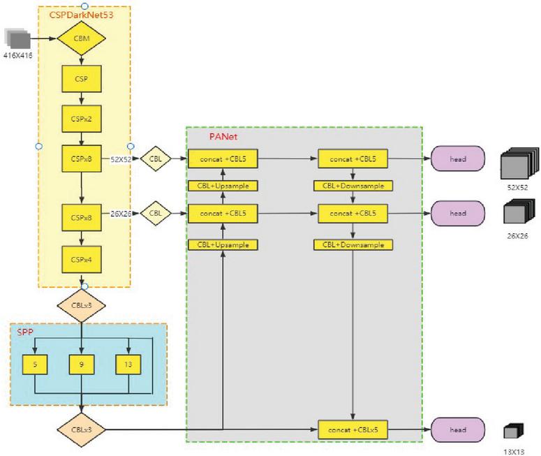
Figure 1 Yolov4 structure diagram.
The convolutional neural network structure consists of Backbone, Neck and Head. It uses CSPDarknet53 as the Backbone, SPP+PANet as the Neck, and the detection head Head follows that of yolov3, as shown in Figure 1.
The images in the batch are resized to 416 416 pixels before entering the convolutional backbone network. It traverses 5 CSP residual convolution blocks, the height and breadth of the feature layers are continually compressed, and the number of channels is increased to produce the last 3 shaped feature layers. The last layer of the feature layer has the broadest perceptual field and the greatest semantic density. It is sent to the SPP module, which sends the sub-feature layer via the 5 5, 9 9, and 13 13 maximum pooling downsampling layers, respectively. It links the outputs of the three branches to the original input concat and feeds them to the PANet module through three CBM convolution layers. The 3 SHAPE feature layers are layered by upsampling from the bottom up, and the 13 13 feature layer is convolved with 26 26 by upsampling and stacking. It then enters the up-sampling layer with 52 52 for stacked convolution, followed by top-down down-sampling stacking to complete the pyramidal feature structure and extract the effective feature information. The three feature layers are sent to the HEAD module [14–16].

Figure 2 Component structure diagram.
The construction of the yolov4 convolutional network plug-in is depicted in Figure 2. The Backbone body is composed on five CSP residual convolutional blocks. The CSP structure is seen in Figure 2(a). The number of Resblock in each convolutional block is 1/2/8/8/4, correspondingly, to enhance the learning ability of the network. Each Resblock backbone component is composed of a 1 1 convolutional block and a 3 3 convolutional block. The leftover edge portion is not processed. Finally, the two components are joined. See Figure 2(b). Figure 2 depicts the three components of the convolutional block CBM: conventional convolutional Conv, BN batch normalization, and Mish activation function (c). The convolution block CBL consists of three components: ordinary convolution Conv, BN batch normalization, and the Leaky Relu activation function (see Figure 2 for further explanation) (d).
3 Improve Yolov4
The original YOLOv4 can provide low detection accuracy, which may lead to a large number of missed detections and incorrect target prediction due to insufficient multiscale feature extraction. Especially in the presence of a large number of small targets and multiple occluded targets, the detection accuracy is poor. YOLOv4 has a high computing cost and long training time, which may not be suitable for on-site mobile devices.
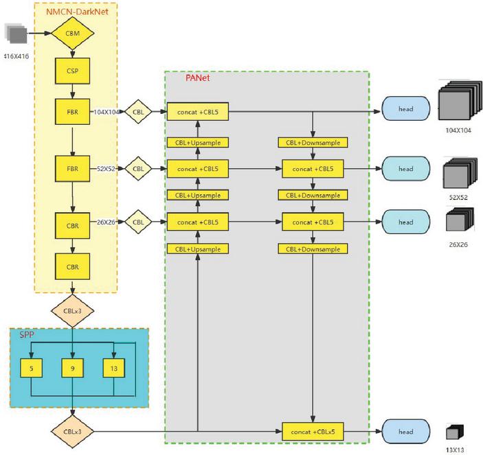
Figure 3 Structure of the optimized convolutional network.
Figure 3 shows how we enhanced the yolov4 method and proposed an improved FBR-yolov4 algorithm in this study. The residual module is optimized first. The original residual module is incapable of extracting enough features. To increase the capability of backbone network feature extraction, a novel form of small-block, multi-batch residual convolution module is presented. Second, the FSM feature separation module is presented to increase the breadth of the convolutional layer and enhance network accuracy. The third step is to establish an attention mechanism. To suppress the invalid features, a lightweight module CBAM is introduced to the NBR convolutional block, strengthening the effective features and further improving the feature extraction capability of the original network. Fourth, the original network is insufficiently accurate for detecting tiny targets. The second layer feature layer of the backbone network is added into the deep feature fusion network to improve the PANet network layer feature fusion. Fifth, the original network’s speed is increased. The Mish activation function is replaced with the lightweight H swish activation function.
3.1 Batch Residual Convolution Module (BR)
Deep learning has advanced tremendously since the introduction of the residual module. The typical convolutional neural network transferring information is going to lose some information, and information loss does occur. As the depth of a convolutional neural network continues to grow, gradient disappearance will occur to prevent convergence. Moreover, when the network is deeper past a certain point, too much information is lost, making it harder to increase the network effect or, worse, resulting in network deterioration. However, it is inevitable to deepen the network in order to enhance the accuracy of the convolutional network in order to discover more finer characteristics. The incorporation of residual modules can not only mitigate the gradient disappearance, but the continual mapping capability of residual modules can enable the deeper network to attain at least the same level of characterisation capability as the shallow network. Figure 4 illustrates the construction of the batch residual module (BR) presented in this study (a). First, it separates the input batch picture into four according on the number of channels, and then it sends the entire batch image to the CBM convolution block. The convolution kernel has a 3 3 dimension and a 1 pixel step size. After concat, the result is convolved with a quarter of the input picture, and the summing operation is conducted on the feature layer. The above steps are continued until each of the original image’s four components has been added to the convolution. The number of channels doubles at this moment.
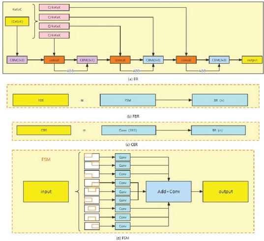
Figure 4 Component structure diagram.
3.2 Improvement of FPNet Module
Deeper network feature maps provide more resolution in convolutional neural networks. It can more accurately depict the image’s characteristics and textures. Therefore, it is more appropriate for detecting little things. Nevertheless, the shallow network traverses fewer convolutional layers and is more vulnerable to noise interference; accordingly, the recovered semantics are limited. The deeper network has a lower resolution and a broader perceptual field per feature. Therefore, it has a greater amount of semantic information and a more exhaustive representation of the total image information. In contrast, it is not conducive to the identification of little objects. 52 52 feature layer each pixel point corresponds to a pixel grid of 8 8 in the original picture, and under actual road conditions, objects that are far away from the camera can easily fall below this precision. Lack of information might easily lead to missed detections. It is a clear deficiency of convolutional networks that must identify a large number of tiny and obscured objects. 104 104 feature layers are implemented in order to improve accuracy and compensate for the weaknesses of shallow and deep networks. In addition, the unit pixel point should match to a 4 4 pixel grid of the original picture in order to increase the precision of tiny target recognition and reduce the number of missed detections.
In order to improve the accuracy of the detection of small object targets and occlusion targets, in addition to the basic three feature layer structure consisting of 13 13, 26 26, and 52 52, the 104 104 feature scale feature layer is additionally added to the FPNet network in order to enhance the feature extraction effect. In the feature fusion layer, the output of the FBR module found in the third layer of the backbone network is convolved. Following that, the results of the 52 52 upsampling layer are concatenated with those of the CBL5 convolution module. Figure 5 depicts the CBL5 sub-convolution module in its entirety. After that, the downsampling operation is carried out in order to accomplish the refined feature fusion process by fusing it with the 52 52 feature layer. The fused 52 52 feature layers are then input through the CBL5 convolution, and the appropriate feature layers are then sent into the neck structure for the further procedures.
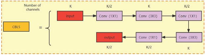
Figure 5 CBL5 structure diagram.
3.3 CBAM
Over the course of the past few years, attention mechanisms have become an increasingly prevalent tool in target identification. It has been demonstrated to enhance the performance of target detection convolutional networks. The formation of attention is fundamentally dependent on the attention mechanism communicating to the network the locations within it that require attention. There are three distinct types of network domains that may be differentiated based on the target of the network’s attention: the geographical domain, the channel domain, and the hybrid domain respectively.
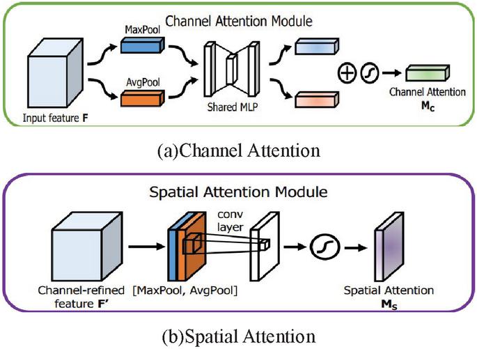
Figure 6 Channel, spatial attention mechanism module.
This paper presents the CBAM attention module for further study. CBAM is a hybrid domain mechanism module that combines the functionality of the Spatial Attention Module and the Channel Attention Module mechanism modules. As a result of this combination, CBAM is able to better balance both sides and provide a higher level of performance for the network.
The spatial dimension of the feature map is compressed by the Channel Attention module. The structure is seen in Figure 6(a). It is comprised of two parts. A portion is allocated to the averaging pool layer. It passes via the 1 1 convolution layer, where the channel is decreased to 1 in 16 and the ReLU activation function is used to activate the image. The remaining portion enters the layer of greatest pooling. It is subjected to 1 1 convolution, the number of channels is lowered to one in sixteen, and the ReLU function is activated. After sigmoid activation and a summing operation with the preceding section, the weights are normalized. The output feature map is then multiplied by the input feature map to produce the channel attention feature map. In the spatial domain, the output of the Channel Attention module is processed. The module is seen in Figure 6(b). It applies maximum pooling and average pooling of channel dimensions, respectively, to the input feature map before concatenating the two sections of the output. After sigmoid activation, the input feature maps are multiplied by the normalized weights and then the result is produced [16–18].
3.4 FSM Feature Separation Module
Network performance improves to a certain extent as network depth grows. However, the depth is too great, which leads to gradient instability, network degeneration, and a lengthy training and validation period. Consequently, this research examines one additional parameter, breadth. The breadth allows each network layer to get a deeper understanding of visual aspects and nuances. If the network width is too thin, the data gathered at each layer is insufficient. Even with a deep network, it is challenging to get good performance. Expanding the width leads to an exponential rise of computation, therefore increasing the width is not an advantage [17].
In this research, we present the feature separation module, which divides the input feature map into nine parts and performs a convolution operation to lower the feature scale and achieve width expansion, respectively. In the output following feature fusion, the feature size of the output feature map is half of the feature scale of the input feature map, and the number of channels remains the same. Figure 4 depicts the module structure for feature separation (d).
3.5 The h-swish Activation Function
The H-swish function is an alternative form of the swish function. It has been demonstrated that the swish is a highly effective activation function. Due to the introduction of the sigmiod function in the swish function, which is more difficult to compute, h-swish is recommended to replace the Mish activation function in the network in order to minimize the computing effort and lighten the network [18].
The function expression for swish:
| (1) |
Function expressions for h-swish:
| (2) |
The curve are shown in Figure 7.
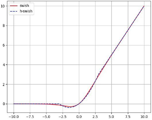
Figure 7 Swish, h-swish curves.
4 Experimental Simulation and Performance Analysis
4.1 Experimental Environment
The experimental training environment of this article is shown in Table 1. The CPU is AMD EPYC7601, the GPU is RTX3090, the memory is 32G, the operating system is Ubantu 20.04, the python version is 10.1, the Cuda version is 11.1.1, and the python version is 3.8. The experimental verification environment is shown in Table 2. The CPU is AMD R7 4800H, the GPU is 1650Ti, the memory is 16G, the win10 operating system, the python version 10.1, the Cuda version 11.1.1, and the python version 3.8.
Table 1 Training environment
| Item | Version |
| CPU | AMD EPYC 7601 |
| GPU | NVIDIA GeForce RTX 3090 |
| memory size | 32G |
| system | Ubantu20.04 |
| Pytorch | 10.1 |
| Cuda | 11.1.1 |
| Python | 3.8 |
Table 2 Experimental validation environment
| Item | Version |
| CPU | AMDRyzen 7 4800H |
| GPU | NVIDIAGeForce RTX 1650Ti |
| Memory size | 16G |
| System | Windos10 |
| Pytorch | 10.1 |
| Cuda | 11.1.1 |
| Python | 3.8 |
4.2 Experimental Data Set
In this paper, the large driving data set BDD100K published by the AI laboratory of Berkeley University is used as the data set of this experiment. The scene of this data set is complex and the target detection is difficult.
There are 80000 driving picture data in total, with the image resolution of 1280 720, the data volume of training set is 70000, and the data volume of verification set is 10000. See Figure 8 for the labeled data volume of each category.
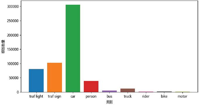
Figure 8 Map of the number of label.
4.3 Anchor
In this paper, K-Means clustering is used to train the label boxes to be trained for all data sets, and the anchor box suitable for the data set is obtained. There are four detection layers in this paper, and anchor is selected. The number of boxes is 12. The K-Means clustering result is shown in Figure 9, and the prior frame size is [3,5], [4,8], [3,15], [6,12], [9,8], [11,16], [7,27], [15,26], [26,32], [36,53], [63,80], [108,158].
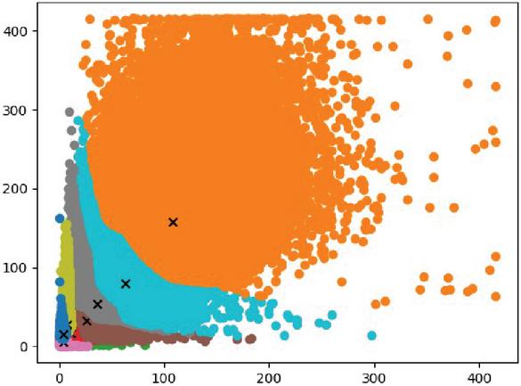
Figure 9 k-means.
4.4 Evaluation Indicators
As assessment measures, this paper cites AP (Average Precision) and FPS (Frames Per Second). AP represents the region bounded by the precision and recall curves (P-R curve). P evaluates the accuracy of prediction. R assesses prediction recall, and the formulas for AP, P, and R are as follows:
| (3) | ||
| (4) | ||
| (5) |
Where represents the number of targets properly detected by the model, represents the number of targets wrongly detected, represents the number of targets overlooked by the model, and represents the number of targets recognized by the model that do not fall into this category.
4.5 Comparative Experiment
On this dataset, comparative tests of each method are performed to illustrate the advancedness of the upgraded algorithm. According to Table 3, the improved method in this study has good AP values for both the Car and Truck categories at input sizes of 416 416 and 640 640, respectively. The Bus category, on the other hand, is somewhat worse. This is thought to be due to a lack of annotated information in the bus category as well as a lack of a balanced data collection. By raising the weight of the bus category, the accuracy of the bus category may be increased. In this study, we can observe that the method obtains the maximum mAP when compared to other good algorithms, indicating that it is advanced.
Table 3 BDD100K dataset comparison experiments
| Input | Category AP/% | mAP/% | |||
| Model | Size | Car | Bus | Truck | |
| Yolov4 [7] | 416 416 | 65.16 | 42.38 | 46.04 | 51.19 |
| Yolov4 [7] | 640 640 | 61.35 | 56.92 | 53.71 | 57.32 |
| DR-YOLOv4 [19] | 640 640 | 62.23 | 58.07 | 54.42 | 58.24 |
| Yolov5s | 640 640 | 71.40 | 55.50 | 48.90 | 58.60 |
| CAM-YOLO [19] | 640 640 | 76.20 | 58.74 | 47.00 | 60.60 |
| ous | 416 416 | 73.88 | 49.15 | 54.40 | 59.14 |
| ous | 640 640 | 75.68 | 51.46 | 56.76 | 61.30 |
4.6 Results and Analysis of Ablation Experiments
Ablation experiments are built and performed using the BDD100K dataset to validate the usefulness of modules such as BR and FSM proposed in this study. The input size is 416 416, and the test results are provided in Table 4.
Table 4 Dataset test results
| Category AP/% | All | |||||||
| Model | Car | Bus | Truck | AP | FPS | Categories AP | Precision | Recall |
| Baseline | 65.16 | 42.38 | 46.04 | 51.19 | 24 | 38.9 | 75.35 | 32.3 |
| Baseline+BR | 72.82 | 47.68 | 52.93 | 57.81 | 18 | 42.2 | 76.18 | 30.84 |
| +CBAM | ||||||||
| Baseline+FSM | 73.88 | 49.15 | 54.4 | 59.14 | 18 | 43.86 | 76.66 | 32.4 |
| +BR+CBAM | ||||||||
| Baseline+FSM | 73.24 | 49.16 | 54.16 | 58.85 | 21 | 43.66 | 76.58 | 32.32 |
| +BR+CBAM | ||||||||
| +H-swish | ||||||||
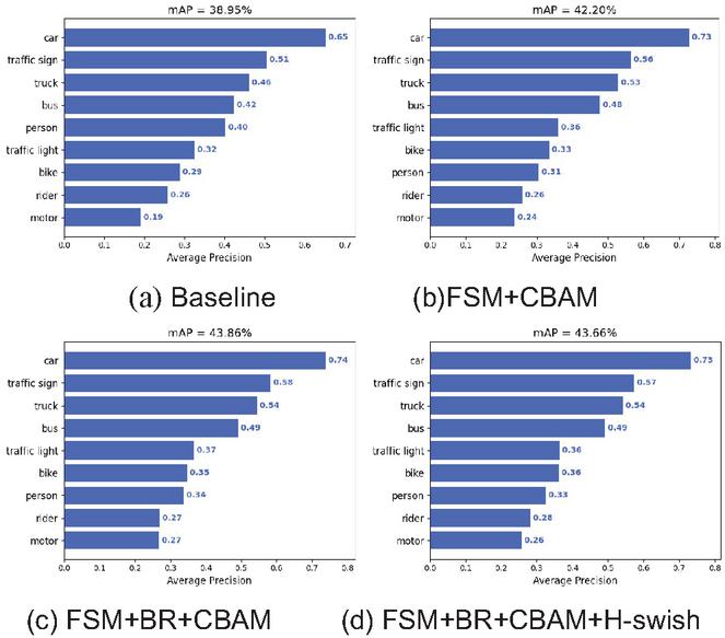
Figure 10 Results of mAP for each network.
The AP value when the yolov4 base model was applied was 38.9, as shown in Table 4. The AP value increases by 3.3 percentage points to 42.2 with the implementation of the BR and CBAM structures. The AP value increases by 4.96 percentage points above the initial value once the FSM module is added, to 43.86. A better balance between speed and accuracy is achieved once the mish activation function is replaced with the h-swish activation function. The AP decreases by 0.2 points while the FPS increases by 3 points. Figures 10(a), 10(b), 10(c), and 10(d) depict the original Yolov4 APs for each category, the BR+CBAM APs for each category, the FSM+BR+CBAM network APs for each category, and the FSM+BR+CBAM+H-swish network APs for each category (d). Notably, all categories – aside from the person category – are improved by the optimized convolutional network, particularly the car category, which is improved by 8, 9, and 8 points, respectively; the traffic sign category, which is improved by 5, 7, and 6 points; the truck category, which is improved by 7, 8, and 8 points; and the bus category, which is improved by 6, 7, and 7 points. When comparing the BR+CBAM network to the FSM+BR+CBAM network, we can see that the AP value of each category has slightly increased as a result of the addition of the FSM module. Because they have fewer tags and smaller targets, people, bikes, riders, and motors in particular benefit more from this improvement.
When comparing the optimized network’s average recall rate to those obtained for the original yolov4 network, it is discovered that there is not a substantial improvement. This problem is addressed by viewing and displaying in the accuracy and recall for each category of the original and improved networks. The categories of person and traffic light are shown to have lower average recall rates. In contrast, all other categories have shown some improvement. At the same time as it is apparent that there is a large rise in remember for all categories at low Score Threshold, it should be noted that the total increase in recall is not very significant. This demonstrates that the optimized network recalls more targets than the unoptimized network. Due to the confidence level not being high enough to be discounted, it is not reflected. It is plausible to surmise that the optimized network performs better than anticipated with a greater number of labels given that the dataset categories utilized in this article are not sufficiently balanced.
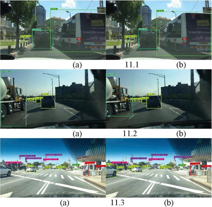
Figure 11 Data set image detection effect comparison diagram.
4.7 Effectiveness of Target Detection
In Figure 11, the left figure shows the detection results of the original network model, and the right figure shows the detection results of the optimized model. Among them, Figure 11.1(a) multiple vehicle occlusions on the left side have missed detection. Figure 11.1(b) identifies the missed vehicles. Figure 11.2(a) There is also a missed detection when the vehicle is obscured. Correction is also made in Figure 11.2(b). Figure 11.3(a) Multiple misses exist on the left side. Figure 11.3(b) shows the reduction of missed detections. The optimized network detection is significantly better. Experimental results show that the detection effect for multiple occluded targets and small targets is better.
5 Conclusions
In this study, we increase the detection impact of tiny targets and obscured targets under real-time road circumstances for the absence of effect. Backbone network is intended to be FBR-DarkNet, and the CBAM attention mechanism is added into the backbone network to increase the convergence speed and to boost the network aggregation capabilities. In order to improve the performance of the network with regard to the identification of tiny targets, the number of layers of feature fusion module input has been increased. The k-means clustering technique is used to the dataset in order to produce specific a priori frames. This work has a strong performance for detecting road objects, with a significant improvement in accuracy on all different kinds of cars. This is an important contribution to the field. It performs pretty well when compared to other popular algorithms. While this is true, there is still a significant amount of untapped potential for growth and development within the Yolo series. Research in the future may continue to investigate convolutional networks that are more accurate and efficient for it, and may also seek to improve the network’s performance by employing knowledge distillation techniques [20], etc.
Acknowledgments
National Natural Science Foundation of Shandong Province (ZR2017BF043).
References
[1] Girshick. R. Fast r-cnn[C] Proceedings of the IEEE international conference on computer vision. 2015:1440–1448.
[2] Yang S, Wang J, Hu L, et al. Research on improved Retina-Net’s occlusion target detection algorithm[J]. Computer Engineering and Applications, 2022, 58(11): 209–214.
[3] Jia K C, Ma Z H, Zhu R, et al. Attention mechanism to improve lightweight SSD model for sea surface small target detection[J]. Chinese Journal of Image Graphics, 2022, 27(04):1161–1175.
[4] Gu Yongli, Zong Xinxin. A review of deep learning-based target detection research[J]. Modern Information Technology 2022, 6(11):76–81. DOI: 10.19850/j.cnki.2096-4706.2022.011.020.
[5] Hou Xueliang, Shan Tengfei, Xue Jingguo. Analysis of typical algorithms for target detection with deep learning and its application status[J]. Foreign Electronic Measurement, 2022, 41(06):165–174.
[6] Zheng Hao, Liu Jianfang, Ren Xiaogang. Dim Target Detection Method Based on Deep Learning in Complex Traffic Environment [J]. Journal of Grid Computing, 2022, 20(1).
[7] Bochkovskiy Alexey, Wang C Y, Liao H Y M. YOLOv4: optimal speed and accuracy of object detection[J]. arXiv preprint, 2020, arXiv:2004.10934.
[8] Wenhao Cao, Zhuoyu Feng, Dongyao Zhang, et al. Facial Expression Recognition via a CBAM Embedded Network[J]. Procedia Computer Science, 2020, 174.
[9] Huang Shan, He Ye, Chen Xiao-an. M-YOLO: A Nighttime Vehicle Detection Method Combining Mobilenet v2 and YOLO v3[J]. Journal of Physics: Conference Series, 2021, 1883.
[10] Wang C Y, Liao H Y M, Wu Y H, et al. CSPNet: A new backbone that can enhance learning capability of CNN[C]//Proceedings of the IEEE/CVF conference on computer vision and pattern recognition workshops. 2020: 390–391.
[11] He K, Zhang X, Ren S, et al. Spatial pyramid pooling in deep convolutional networks for visual recognition[J]. IEEE transactions on pattern analysis and machine intelligence, 2015, 37(9).
[12] Liu S, Qi L, Qin H, et al. Path aggregation network for instance segmentation[C]//Proceedings of the IEEE conference on computer vision and pattern recognition. 2018: 8759–8768.
[13] Ju Zhiyong, Li Yuming, Xue Yongjie, et al. Pedestrian detection algorithm based on improved YOLOv4 model[J/OL]. Control Engineering:1–13 [2022-10-26]. DOI: 10.14107//j.cnki.kzgc.20220053.
[14] Mahto P., Garg P., Seth P, et al. Refining Yolov4 for vehicle detection[J]. International Journal of Advanced Research in Engineering and Technology, 2020, 11(5).
[15] Chen Zhixiong, Tian Shengwei, Yu Long, et al. An object detection network based on YOLOv4 and improved spatial attention mechanism[J]. Journal of Intelligent & Fuzzy Systems, 2022, 42(3).
[16] Ren, Feng Yi, Pei, Xinbiao, Qiao, Zheng, et al. A lightweight detection method for YOLOv4 incorporating CBAM[J/OL]. Small Microcomputer Systems:1–8 [2022-10-26]. http://kns.cnki.net/kcms/detail/21.1106.tp.20220301.0935.002.html
[17] Zhao Qi. Mobile Net-V3-based fatigue driving detection algorithm [D]. Hangzhou University of Electronic Science and Technology, 2022. DOI: 10.27075/d.cnki.ghzdc.2022.000209.
[18] Evan, Wulandari Meirista, Syamsudin Eko. Recognition of Pedestrian Traffic Light using Tensorflow And SSD MobileNet V2[J]. IOP Conference Series: Materials Science and Engineering, 2020, 1007 (1).
[19] Deng T M, Liu X H, Wang L et al. A vehicle detection algorithm combining cascaded attention mechanism[J/OL]. Computer Engineering and Applications:1–12 [2022-11-11]. http://kns.cnki.net/kcms/detail/11.2127.TP.20220926.2015.020.htm.
[20] Hinton G, Vinyals O, Dean J. Distilling the knowledge in a neural network[J]. arXiv preprint arXiv:1503.02531,2015.
Biographies
Qinghe Yu received the bachelor’s degree from Dalian Polytechnic University in China in 2019. Currently, he is a graduate student in the School of Information and Control Engineering, Qingdao University of Technology, China, majoring in computer science and technology, and his research direction is deep learning.
Huaiqin Liu In 2020, he received a bachelor’s degree in computer science and technology from Qingdao University of Science and Technology. He is currently studying for a master’s degree in the School of Information and Control Engineering, Qingdao University of Technology. His research areas include deep learning.
Qu Wu received the bachelor’s degree from Northeast Forestry University in China in 2006, the master’s degree in Computer application technology from Northeast Forestry University in 2010, the philosophy of doctorate degree in Information engineering from Northeast Forestry University in 2013, respectively. Currently, she is an associate professor of the School of Information and Control Engineering, Qingdao University of Technology, China. Her research fields include reinforcement learning and deep reinforcement learning.
Journal of ICT Standardization, Vol. 11_2, 197–216.
doi: 10.13052/jicts2245-800X.1125
©2023 River Publishers