Standardized Framework for AI-Enabled Decision Support Systems for Sustainable Sports Facility Management: IoT Data Chain Interoperability, Resilience Assessment, and Cognitive Analysis
Rui Zhang1 and Yang Jiang2,*
1Anhui Vocational College of Defense Technology, Lu’an 237005, China
2Anhui Sports Vocational and Technical College, Hefei 230051, China
E-mail: zjdgwh@139.com; jiangyangbj@126.com
*Corresponding Author
Received 16 November 2025; Accepted 19 April 2026
Abstract
In current sports facility management, the lack of unified IoT data standards and the semantic fragmentation of multi-source heterogeneous data make it difficult for AI decision support systems to form a consistent and effective data foundation. This paper proposes a graph neural network (GNN) model based on cross-modal semantic alignment. Taking multi-source sensor data as input, it maps heterogeneous data to a shared semantic embedding space through a unified encoding mechanism. A heterogeneous graph structure is constructed based on device topology and functional coupling. Under the guidance of a graph attention mechanism, weighted propagation and fusion of semantic information between nodes are completed. Simultaneously, contrastive learning constraints are introduced to compress the representation distance between semantically similar nodes, thereby achieving semantic consistency reconstruction of cross-system data chains. Finally, a unified feature representation is output to support upper-level decision analysis. Experimental results show that the system’s interoperability consistency score improves from 0.52 to 0.89, cumulative probability increases from 0.30 to 0.82 when the alignment error is 0.2, and semantic alignment accuracy reaches 92.4%, indicating that the proposed method achieves significant improvements in cross-system data semantic consistency reconstruction and feature representation capabilities. Research shows that this method provides a feasible path for data chain integration and intelligent decision-making in sustainable sports facility management.
Keywords: Sustainable sports facility management, Internet of Things data interoperability, graph neural network, cross-modal semantic alignment, AI-driven decision support.
1 Introduction
Against the backdrop of the ongoing advancement of “dual carbon” goals and smart cities, the green and intelligent transformation of public infrastructure has become an important research direction [1, 2]. As a typical high-energy-consuming and high-frequency-use space, the operational status of sports facilities directly affects the energy consumption structure and public service efficiency [3, 4]. The widespread deployment of IoT technology enables the continuous collection of equipment operation data, environmental parameters, and pedestrian flow information, providing a basic support for data-driven management [5, 6]. Artificial intelligence methods are gradually being applied to the fields of building operation and maintenance and energy management, promoting the transformation from traditional experience-based decision-making to intelligent decision-making [7, 8]. Sustainable sports facility management not only involves energy conservation and emission reduction but also relates to system stability and service continuity. Its complexity has prompted research to move from single optimization to system-level collaboration [9, 10]. Decision support systems oriented towards multi-source data fusion and intelligent analysis have become an important research direction [11, 12].
Current sports facility management faces multi-dimensional technical challenges at both the data and system levels. Significant differences exist between multi-source IoT devices in terms of protocol standards, data structures, and semantic representation, resulting in heterogeneous data even during the acquisition phase [13, 14]. The lack of a unified description mechanism in data chain transmission and storage makes it difficult to establish consistent data interfaces between different systems [15, 16]. Spatial topology and functional coupling exist between devices, but these relationships are not effectively modeled, making it difficult to express the correlation information between data [17, 18]. Noise interference and missing data in real-time data streams further weaken data quality and reliability [19, 20]. Existing management systems typically employ a distributed architecture, with each subsystem operating independently, lacking a unified semantic space, making it difficult for upper-level analysis models to directly integrate multi-source data [21, 22]. These problems collectively lead to decreased data utilization efficiency and limited decision support capabilities.
To address these issues, existing research has proposed various solutions. Modeling methods based on BIM and digital twins integrate equipment and spatial information by constructing virtual-real mapping relationships, but these methods rely on stable data interfaces and unified data formats, leading to semantic inconsistencies in multi-source heterogeneous environments [23, 24]. Optimization methods based on machine learning and reinforcement learning have made progress in energy consumption prediction and control scheduling, but their training process relies on high-quality data input and is mostly concentrated in a single system, lacking cross-system data fusion capabilities [25, 26]. Data-driven methods for IoT architecture achieve data acquisition and processing through layered design but, in the data fusion stage, they remain at the structural alignment level and have not established a unified semantic expression mechanism [27, 28]. Graph model methods are used to describe the relationship structure between devices, but most studies focus on topological connections without introducing semantic constraint mechanisms, making it difficult to solve the semantic fragmentation problem [29–30]. Existing methods have structural gaps between unified data expression and intelligent analysis, making it difficult to build a unified and effective AI decision support system.
To address the issues of insufficient interoperability and semantic inconsistency in IoT data chains, this paper proposes a graph neural network (GNN) method for cross-modal semantic alignment. Raw multi-source data is mapped to a shared semantic embedding space through a unified encoding function, where initial alignment of different data types is achieved. A heterogeneous graph structure is constructed based on the spatial location and functional relationships of devices, embedding the semantic information of nodes and edges into the graph topological representation. Weighted feature propagation and fusion between nodes are achieved under the action of a graph attention mechanisms. Contrastive learning constraints are introduced to reconstruct the embedding space distribution by optimizing the distance relationships between semantically similar samples, thereby eliminating semantic inconsistencies in the data chain. Finally, a unified feature representation is formed and output to the decision support layer, realizing the connection from data collection to intelligent analysis. This method forms a unified technical path in heterogeneous data semantic modeling, graph structure relationship representation, and consistency optimization, providing a stable data foundation and analytical support for sustainable sports facility management.
2 Method
2.1 System Overall Architecture and Unified Data Link Representation Mechanism
A standardized framework for an AI-enabled decision support system for sustainable sports facility management is established. Its unified data chain representation mechanism is implemented based on the overall system architecture. This architecture clearly defines end-to-end processing specifications for multi-source IoT data, ranging from the acquisition layer to the decision layer. This includes real-time acquisition of raw sensor signals, data cleaning and timestamp alignment, cross-modal semantic embedding and encoding, heterogeneous graph structure construction, graph attention information propagation, contrastive learning optimization, and unified feature output.
Modules interact through standardized data interfaces that define data formats, dimensional transformation rules, and transmission protocols. This ensures consistent interoperability of data flows between devices from different manufacturers and heterogeneous systems.
Let the original multi-source sensor dataset be , where represents the original data vector of the -th sampling point, and is the total number of sampling points. A unified representation mechanism defines a mapping function that maps the original data space to a shared semantic embedding space , where d denotes the embedding dimension. This mapping satisfies the semantic fidelity condition under the invertibility constraint, as shown in Equation (1):
| (1) |
where is the nonlinear feature extraction function, is the learnable weight matrix, is the dimension of the extracted feature , and is the bias term. The mapped embedding vector retains the device type, spatiotemporal label, and functional attributes, forming the basic expression unit of the unified data chain. The overall system architecture and data flow relationship between modules are shown in Figure 1.
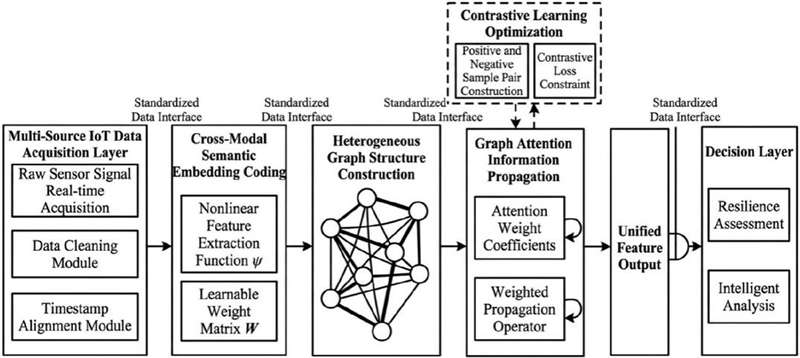
Figure 1 Overall architecture and data-flow process of the AI-enabled decision-support framework for sustainable sports facility management.
Figure 1 presents the overall architecture and data-flow logic of the proposed AI-enabled decision-support framework for sustainable sports facility management. The framework begins with a multi-source IoT data acquisition layer, where raw sensor signals are collected in real time and processed through data cleaning and timestamp alignment. The standardized data interface then transfers the preprocessed data to the cross-modal semantic embedding module, in which nonlinear feature extraction and learnable transformation are used to convert heterogeneous sensor inputs into a unified representation space.
Based on the embedded features, a heterogeneous graph structure is constructed to model the relationships among devices, spatial locations, temporal states, and functional attributes. Graph attention-based information propagation is subsequently applied to estimate the relative importance of different nodes and edges, enabling weighted feature aggregation across the system. To further enhance representation robustness, contrastive learning optimization is incorporated by constructing positive and negative sample pairs and applying contrastive loss constraints. The resulting unified feature output is then delivered to the decision layer, supporting resilience assessment and intelligent analysis for facility operation and management.
2.2 Cross-Modal Semantic Embedding Modeling of Multi-Source Heterogeneous Data
To address modal differences and semantic gaps in the original feature spaces of multi-source heterogeneous sensor data in sports facilities, a cross-modal semantic embedding model is constructed to obtain a unified representation. Let denote the -th observation sample from the -th data source or modality, where is the original feature dimension of that modality. A modality-specific encoding function is defined as , which maps heterogeneous input features into a shared semantic embedding space. The mapping relationship is formulated as follows:
| (2) |
where denotes the cross-modal semantic embedding vector of the -th sample from the -th modality, is the modality-specific learnable weight matrix, is the bias vector, is the nonlinear activation function, is the unified embedding dimension, and represents the trainable parameter set of the -th encoder. Through this transformation, heterogeneous data from different modalities are projected into the same semantic space while retaining modality-specific information related to device attributes, temporal patterns, spatial locations, and operational states.
All embedding vectors constitute a point set in the shared semantic space. Their spatial distribution reflects the semantic similarity, aggregation tendency, and dispersion characteristics of different source data after cross-modal mapping. The resulting semantic embedding distribution of multi-source heterogeneous data is shown in Figure 2.
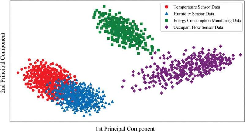
Figure 2 Two-dimensional PCA visualization of multi-source sensor data after cross-modal semantic embedding.
Figure 2 visualizes the distribution of multi-source sensor data in the shared semantic embedding space after cross-modal mapping. To facilitate interpretation, the high-dimensional embedding vectors are projected onto the first two principal components. The temperature and humidity sensor data show partial overlap, indicating that these two environmental modalities share certain correlated temporal and operational characteristics. In contrast, the energy consumption monitoring data form a relatively independent cluster, suggesting that energy-related features contain distinct semantic information compared with environmental sensing signals. The occupant flow sensor data are distributed in a separate band-like region, reflecting their stronger association with spatial usage intensity and dynamic facility occupancy patterns.
Overall, the distribution demonstrates that the proposed cross-modal semantic embedding model can project heterogeneous sensor inputs into a unified representation space while preserving modality-specific differences. The clear separation among most clusters indicates that the learned embeddings retain discriminative information across different data sources, whereas the partial overlap between temperature and humidity data reflects their natural physical correlation. This result supports the feasibility of using the unified embedding representation for subsequent heterogeneous graph construction and graph attention-based semantic relation propagation.
2.3 Semantic Relation Propagation Model Based on Graph Attention Mechanism
After cross-modal semantic embedding is mapped to the shared space, the device topology relationship and functional coupling dependency between the sensing nodes, actuator nodes, and functional unit nodes in the sports facility constitute the basic edge definition of the heterogeneous graph structure. The node set contains various types, and the edge set is constructed according to the physical connection of the device, spatial proximity, or functional cooperation relationship to form a heterogeneous graph , where represents the set of all nodes (such as data acquisition nodes, status monitoring nodes, control nodes), and represents the set of edges between nodes (such as communication links, spatial adjacency relationships, or functional cooperation relationships). Each node carries an initial feature vector from the shared semantic embedding space , where represents the dimension of the embedding vector and is the feature representation of the node in the initial layer. In order to capture the differential contribution of different neighboring nodes to the semantic update of the target node, a graph attention mechanism is introduced to calculate the attention weight of each node’s neighborhood (including itself). The attention coefficient of node to node is calculated by a feedforward neural network, which takes the node features after linear transformation as input, as shown in Equation (3):
| (3) |
where is a learnable linear transformation matrix that maps the input features from to a higher-dimensional latent space ; and are the feature vectors of node and node in the layer respectively; represents the vector concatenation operation, with the concatenated dimension being ; is a learnable attention parameter vector, whose transpose is the dot product of the concatenated vector; LeakyReLU is a non-linear activation function used to introduce small gradients in the negative range. The final attention weights are obtained by normalizing the results of all neighbors of the node using SoftMax, as shown in Equation (4):
| (4) |
where the numerator is the exponential form of the attention coefficient of the node, and the denominator is the sum of the exponential coefficients of all the node’s neighbors, ensuring that the sum of all weights is 1. The normalized weights measure the relative importance of neighboring nodes to the semantic update of the node during the aggregation process . The feature representation of the node at the 1st layer is obtained by weighted aggregation of neighboring features and nonlinear transformation, as shown in Equation (5):
| (5) |
where is a nonlinear activation function (using ELU), which acts on the weighted summation result; is the attention weight calculated by Equation (2); W shares the same parameters as the transformation matrix in Equation (1); is the feature vector of the neighbor node in the layer; summation iterates through all neighbors of the node . This propagation process is stacked between multiple graph attention layers and, after each layer is updated, the node features gradually integrate semantic information from more distant neighbors. The attention parameters and transformation matrices W corresponding to different a edge types in the heterogeneous graph are learned independently to adapt to the semantic propagation characteristics under different relational patterns. After multiple layers of propagation, each node obtains enhanced semantic features that integrate topological structure and functional coupling relationship. Figure 3 shows the distribution of attention weights among nodes in the graph structure. The color depth reflects the normalization coefficient on different edges, thus intuitively presenting the adaptive propagation path and gathering hotspots of semantic information in the network.
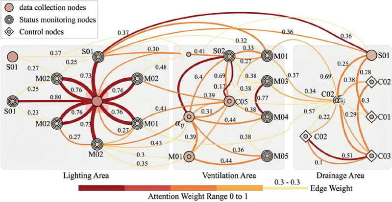
Figure 3 Semantic weight distribution of graph structure.
Figure 3 illustrates the heterogeneous topological relationships and attention weight distribution among nodes within the sports facility. Each circular node represents a device unit, with data acquisition nodes represented by solid circles, status monitoring nodes by concentric rings, and control nodes by diamonds containing smaller circles. All nodes are horizontally divided into three vertical strips based on their respective physical areas (lighting, ventilation, drainage). Within each strip, nodes are arranged vertically according to their spatial installation location, with clear intervals separating the strips. The connecting edges between nodes are drawn as curves. The line width and color depth of each edge jointly encode the corresponding normalized attention weight coefficient . Edges with weight values between 0.7 and 1.0 are 3 pixels deep red, edges between 0.3 and 0.7 are 2 pixels orange, and edges below 0.3 are 1 pixel light yellow. Each edge is also labeled with a weight value rounded to two decimal places. The diagram shows several nodes forming radial clusters where multiple high-weight edges converge. For example, a data acquisition node (S02) in the center of the lighting area is connected to six surrounding status monitoring nodes (M01 to M06) by a thick, dark red edge, with a light red background highlight for this node. All node identifiers use a uniform format: S indicates a data acquisition node, M indicates a status monitoring node, and C indicates a control node. A gradient legend corresponding to the line width is provided below the diagram, with the horizontal axis indicating attention weight values ranging from 0 to 1, accompanied by a description of “edge weight”. A node type legend is displayed in the upper left corner of the diagram, using the same fill pattern as in the diagram. The overall layout clearly shows the dense connection paths formed by high-weight edges, highlighting the main channels for semantic information propagation.
2.4 Contrastive Learning-Driven Semantic Consistency Optimization Mechanism
In the cross-modal semantic embedding space, the initial representation formed after unified encoding of multi-source heterogeneous data still suffers from the problem of scattered features of data of the same type and blurred boundaries of data of different types. To solve this semantic fragmentation, a contrastive learning strategy is introduced to impose structural constraints on the embedding space. For anchor samples in each training batch, a set of positive samples is constructed based on the device type and function category of their original data, that is, samples that share the same semantic label with the anchor. At the same time, all other samples with different semantic labels are regarded as a set of negative samples. The goal of contrastive learning is to bring the anchor and positive samples closer in the embedding space, while pushing the anchor and negative samples further apart, thereby strengthening the clustering of semantically similar data representations. This optimization process is achieved by defining a normalized temperature scale cross-entropy loss function, as shown in Equation (6).
| (6) |
where is the normalized feature vector, represents the cosine similarity function, is the temperature hyperparameter used to adjust the sharpness of the similarity distribution. The union of the positive and negative sample sets in the denominator is summed to ensure the effectiveness of the normalized probability distribution. This loss function forces the similarity between the anchor and the positive sample to be significantly higher than the similarity between the anchor and the negative sample by minimizing the negative log-likelihood. During training, the contrastive learning loss and the main loss of the graph attention network are jointly optimized to update the parameters of the semantic embedding encoder. The constraint driven by contrastive learning causes semantically similar node representations to form compact clusters in the embedding space, while the boundaries between clusters of different semantic categories are clearly separated, ultimately eliminating semantic inconsistencies in the cross-system data chain. Figure 4 shows the convergence distribution of similar samples in the semantic space after contrastive learning optimization, where different colors represent different semantic categories. Intra-cluster distance is significantly reduced and inter-cluster boundaries are clear, indicating that the semantic consistency reconstruction goal has been achieved.
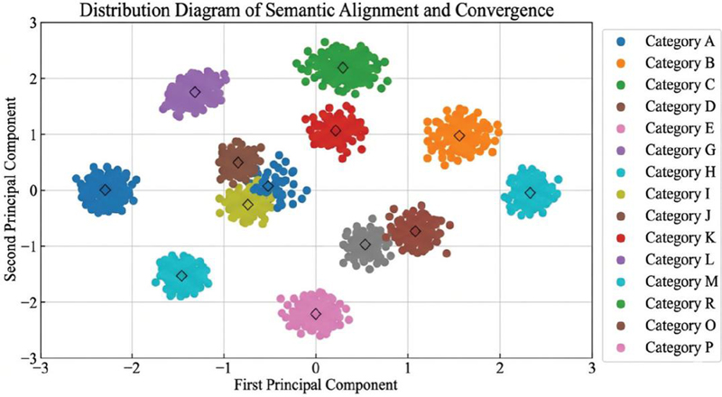
Figure 4 Semantic alignment convergence distribution diagram.
In Figure 4, the horizontal axis of the two-dimensional Cartesian coordinate system represents the first principal component, and the vertical axis represents the second principal component, both ranging from 3 to 3. Figure 4 contains multiple clusters of points of different colors, each color uniquely corresponding to a semantic category. The number of clusters is equal to the total number of semantic label categories in the dataset. Each cluster consists of a large number of densely packed circular data points with minimal Euclidean distance between them, presenting a compact, clumped structure. Clusters of different colors are separated by distinct blank areas, and the boundaries between clusters are clear and non-overlapping. A diamond symbol marks the geometric center of each cluster, serving as the cluster center for that category.
2.5 Unified Feature Output Mechanism for Decision Support
Through semantic information propagation guided by graph attention mechanism and semantic space optimization driven by contrastive learning, multi-source heterogeneous sensor data form semantically consistent feature representations in a shared embedding space. This feature representation exists in the form of heterogeneous graph node embedding matrix, where is the total number of nodes in the graph and is the unified semantic embedding dimension. To support upper-level decision analysis tasks, this embedding matrix needs to be converted into standard interface feature outputs oriented towards specific decision requirements. An output mapping function is defined to aggregate the embeddings of all graph nodes into a fixed-dimensional decision feature vector , where is the decision feature dimension. This mapping process adopts a global attention pooling mechanism, as shown in Equation (7).
| (7) |
where and are learnable linear transformation parameters, is the attention hidden layer dimension. is the attention vector, is the hyperbolic tangent activation function. Through this mechanism, the model performs weighted summation on the features of different nodes in the graph, highlighting the contribution of nodes related to the decision task while suppressing redundant information. The obtained decision feature vector z is connected to a standardized output interface, which defines a unified data format specification, including feature dimension , numerical range normalization interval, and missing value filling rules. Interface output is directly passed to the upper-level decision module to support tasks such as facility operation status assessment, resource scheduling optimization, and resilience quantification analysis. The entire output process does not change the result of semantic consistency optimization but only completes the conversion from graph structure representation to vectorized decision input, ensuring the closure and reproducibility of the data chain.
3 Experiment
3.1 Dataset Construction and Source Description
A multi-source IoT sensor system is deployed in a real sports venue. The acquisition period covered 30 consecutive days of operation in the venue, involving five heterogeneous data sources: environmental monitoring, personnel flow, energy consumption, equipment status, and lighting conditions. Each sensor device synchronously recorded the raw signals at a predetermined sampling frequency. After timestamp alignment and outlier removal, a structured sample set was formed, and the final statistical information is shown in Table 1.
Table 1 Statistics on data acquisition from multi-source heterogeneous sensors
| Data | Sample | Sampling | Deployment | |
| Type | Size | Frequency (Hz) | Device Category | Area |
| Ambient Temperature & Humidity | 120,000 | 1 | Temperature & Humidity Sensor | Zone A/B Stands |
| Personnel Flow | 85,000 | 0.5 | Infrared Pyroelectric Counter | Main Entrance & Aisles |
| Energy Consumption | 200,000 | 10 | Smart Meter | Lighting & Air Conditioning |
| Equipment Operation Status | 45,000 | 0.2 | PLC Status Monitor | Fitness Equipment & Fans |
| Illuminance | 60,000 | 1 | Illuminance Sensor | Functional Areas |
This dataset contains five types of sensor data: ambient temperature and humidity, pedestrian flow, energy consumption, equipment operating status, and light intensity, corresponding to 120,000, 85,000, 200,000, 45,000, and 60,000 samples, respectively. Temperature and humidity sensors, with a sampling frequency of 1 Hz, are deployed in stands A and B of the stadium; infrared pyroelectric counters, with a sampling frequency of 0.5 Hz, are located at the main entrance and various passageways; smart meters, with a sampling frequency of 10 Hz, monitor the energy consumption of the lighting and air conditioning systems; PLC status monitors, with a sampling frequency of 0.2 Hz, are connected to fitness equipment and ventilation fans; and light intensity sensors, with a sampling frequency of 1 Hz, are distributed throughout the venue’s functional areas.
3.2 Experimental Environment and Parameter Settings
In the experimental phase, for the proposed cross-modal semantic alignment GNN, a unified hardware and software operating environment was first built, and the core hyperparameters required for model training were configured based on the PyTorch and DGL frameworks, including semantic embedding dimension, number of graph attention layers, number of multi-head attention heads, optimizer learning rate, batch size, regularization coefficient, temperature coefficient, and sample pair sampling number related to contrastive learning. All parameters were kept consistent in the multi-source heterogeneous data scenario of sports facilities. The specific configuration is shown in Table 2.
Table 2 Core hyperparameter configuration of the proposed model
| Parameter Category | Parameter Name | Parameter Value | Description |
| Embedding Representation | Semantic Embedding Dimension | 256 | Dimension of shared embedding space |
| Graph Neural Network | Number of Graph Attention Layers | 2 | Number of GAT layers |
| Graph Neural Network | Number of Attention Heads | 4 | Number of multi-head attention heads |
| Optimization Strategy | Initial Learning Rate | 1e-3 | Learning rate for Adam |
| Optimization Strategy | Batch Size | 64 | Batch size |
| Regularization | Dropout Ratio | 0.2 | Dropout rate |
| Contrastive Learning | Temperature Coefficient | 0.07 | Temperature for contrastive loss |
| Contrastive Learning | Number of Positive/Negative Pairs | 256 | Number of sampled pairs per batch |
| Training Control | Weight Decay | 5e-4 | L2 regularization coefficient |
Table 2 summarizes the core hyperparameter configuration of the proposed model, including nine key parameters related to embedding representation, graph neural network structure, optimization strategy, regularization, contrastive learning, and training control. The semantic embedding dimension is set to 256. The graph attention network contains two attention layers and four attention heads. For optimization, the initial learning rate is set to , and the batch size is 64. The dropout ratio is set to 0.2 to reduce overfitting, while the temperature coefficient for contrastive learning is set to 0.07. In addition, 256 positive/negative sample pairs are constructed in each batch, and the weight decay coefficient is set to for L2 regularization. These settings are used to support stable model training and effective convergence of the shared semantic embedding space.
3.3 Comparison Methods and Evaluation Indicator Setting
To verify the semantic alignment effect and decision support capability of the proposed model in a multi-source heterogeneous sports facility IoT data environment, the experimental part first constructed a standardized dataset containing attributes such as device type, sampling frequency, and data scale. Then, a unified hardware platform and model training parameters were set, and corresponding experimental tasks and evaluation indicators were designed around five dimensions: data interoperability consistency, semantic alignment accuracy, graph structure information propagation efficiency, semantic consistency optimization degree, and system-level decision response latency. This formed a quantitative test scheme for the output characteristics of each module of the model. The specific configuration is shown in Table 3.
Table 3 Correspondence between experimental tasks and evaluation indicators
| Experiment | Evaluation | Calculation | Corresponding |
| Task | Metric | Method | Output |
| Data Interoperability Consistency | Interoperability Consistency Indicator (IOC) | Mean cosine similarity of feature vectors for same-type data across systems | Unified feature representation layer vector |
| Semantic Alignment Accuracy | Semantic Alignment Accuracy (SAA) | KNN classification accuracy of cross-modal data in shared embedding space | Semantic embedding layer vector |
| Graph Information Propagation | Node Neighborhood Similarity Gain (NSSG) | Improvement rate of mean cosine similarity between node and neighbor representations after graph attention propagation | Graph attention layer node features |
| Semantic Consistency Optimization | Positive-Negative Sample Distance Ratio (PNR) | Ratio of positive pair distance to negative pair distance | Contrastive learning loss function value |
| Decision Response Performance | System-level Decision Response Delay (DRD) | End-to-end average time from raw data input to decision feature output (ms) | Unified feature interface timestamp difference |
Table 3 systematically organizes three core experimental tasks and their corresponding five evaluation metrics. Each task is matched with a specific metric name, computational logic, and model output level. The data interoperability consistency verification task uses an interoperability consistency metric, measuring the output quality of the unified feature representation layer by the mean cosine similarity of cross-system feature vectors. The semantic alignment accuracy evaluation task uses semantic alignment accuracy as a metric, determining the representational capability of the semantic embedding layer based on the K-nearest neighbor classification results of cross-modal data in the shared embedding space. The graph structure information propagation effect evaluation task uses a node neighborhood similarity gain metric to calculate the average similarity improvement rate between the node and its neighboring node representations before and after propagation through the graph attention layer. The semantic consistency optimization effect evaluation task introduces the positive-negative sample comparison distance ratio, reflecting the distance relationship between positive and negative sample pairs in the semantic space through the output value of the contrastive learning loss function. The decision response performance testing task uses a system-level decision response latency metric, measuring the end-to-end time from the original data input to the unified feature interface output.
4 Results
4.1 Data Interoperability Consistency Analysis
To verify the practical effectiveness of the proposed model at the cross-system data fusion level, the experiment selected five typical system pairs in sports facilities (HVAC-lighting, HVAC-security, lighting-security, energy consumption-pedestrian flow, and HVAC-energy consumption). The interoperability consistency scores before and after model processing were compared, and the changes in the cumulative distribution function under different alignment error thresholds were statistically analyzed. Furthermore, the impact trend of different data scales on the consistency index was evaluated. Based on the above experimental design, the data interoperability consistency analysis results are shown in Figure 5.
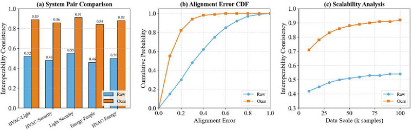
Figure 5 Results of data interoperability consistency analysis: (a) system consistency comparison, (b) cumulative distribution of alignment error, and (c) data scalability analysis.
Figure 5 shows the experimental results for the three subplots. Figure 5(a) is a grouped bar chart, with the horizontal axis representing the five system pairs and the vertical axis representing the interoperability consistency score. The light blue bars represent the original data, and the orange bars represent the data after model processing. The consistency scores of the original data were 0.52, 0.48, 0.55, 0.46, and 0.50, respectively, which improved to 0.89, 0.86, 0.91, 0.84, and 0.88 after processing. The consistency scores of all system pairs improved by more than 0.35. This phenomenon indicates that the model significantly enhanced the level of data interoperability between different systems. This is because the unified semantic embedding and graph attention propagation mechanism effectively eliminated the semantic bias in the original heterogeneous data. Figure 5(b) is a cumulative distribution function plot, with the horizontal axis representing the alignment error and the vertical axis representing the cumulative probability. The light blue curve represents the original data, and the orange curve represents the data after processing. The cumulative probability of the original data at an error of 0.2 was 0.30, which increased to 0.82 after processing; the cumulative probability of the original data at an error of 0.3 was 0.48, which increased to 0.94 after processing. The processed curve approached 1.0 earlier, indicating that the alignment error of most cross-system data pairs was compressed to a lower range. This is because the contrastive learning loss function forces semantically similar node representations to converge, thereby reducing the misalignment distribution of cross-modal features. Figure 5(c) is a line graph, with the horizontal axis representing the data size (in thousands of samples) and the vertical axis representing the interoperability consistency score. The light blue line represents the original data, and the orange line represents the processed data. When the data size increased from 10k to 100k, the original consistency slowly increased from 0.42 to 0.54, while the processed consistency rapidly increased from 0.71 to 0.92. The processed curve consistently lies above the original curve and exhibits a steeper growth slope, demonstrating that the model maintains stable semantic alignment capabilities even with large-scale data. This is because the weighted propagation of the graph attention mechanism can adaptively extend to newly added nodes, while the unified encoding function remains invariant to inputs of different sizes. In summary, the model effectively improves data interoperability across three dimensions: system pairs, error distribution, and data scale.
4.2 Semantic Alignment Accuracy Analysis
To evaluate the effectiveness of the proposed cross-modal semantic alignment mechanism in eliminating semantic fragmentation in the embedding space, a multi-source heterogeneous dataset containing five semantic categories (temperature, humidity, energy consumption, occupancy rate, device status) was constructed. The distribution coordinates of source and target domain samples in the two-dimensional embedding space were recorded before and after alignment, and the classification accuracy of different methods on the semantic alignment task was calculated. By comparing the intra-class clustering and inter-class separation before and after alignment and contrasting the accuracy improvement before and after the introduction of the learning module, the semantic alignment accuracy analysis results are shown in Figure 6.
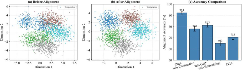
Figure 6 Semantic alignment accuracy analysis results: (a) embedding distribution before alignment, (b) embedded distribution after alignment, and (c) comparison of alignment accuracy of different methods.
Figure 6 shows three subplots. Figure 6(a) is a scatter plot of embedding distribution before alignment. The horizontal and vertical axes represent two dimensions of the embedding space, and different colors represent five semantic categories. Each category contains samples from the source and target domains. The data shows that before alignment the source domain center of the temperature category is located at (3.0, 2.5), while the target domain center is located at (0.5, 2.0). The source domain center (2.0, 1.5) of the humidity category is about 3.0 Euclidean distances away from the target domain center (1.0, 1.0). There is a significant offset between the source domain (1.5, 3.0) and the target domain (3.5, 2.5) of the energy consumption category. The occupancy rate and device status categories also show a separation of source and target domain points. This phenomenon indicates that without semantic alignment, the embedding representation of the same semantic category in different data sources is mapped to different regions in the space, directly resulting in the loss of semantic consistency across the system data chain. Figure 6(b) is a scatter plot of embedding distribution after alignment. The coordinate axes have the same meaning as in Figure 6(a). Data shows that after alignment the source and target domains share centers for temperature (1.2, 2.2), humidity (0.5, 1.2), energy consumption (2.5, 2.8), occupancy rate (1.2, 3.0), and device status (4.0, 0.2). Each color point group is densely packed within itself, and the boundaries between different color point groups are clear. This phenomenon is attributed to the joint constraint of cross-modal semantic embedding and contrastive learning loss: contrastive learning forces semantically similar nodes to shorten their distance in the embedding space, thereby forcing the representations of the same category in the source and target domains to cluster near the shared center. Figure 6(c) is a bar chart with the horizontal axis representing the five methods, the vertical axis representing the percentage of semantic alignment accuracy, and the error bars representing the standard deviation. Data shows that the proposed method achieves an accuracy of 92.4% with a standard deviation of 1.2%; the ablation model without contrastive learning achieves an accuracy of 78.0% with a standard deviation of 2.1%; the ablation model without graph attention achieves an accuracy of 81.3% with a standard deviation of 1.8%; the original feature concatenation model without cross-modal semantic embedding achieves an accuracy of 65.2% with a standard deviation of 2.5%; and the traditional CCA method achieves an accuracy of 70.5% with a standard deviation of 2.0%. The proposed method outperforms the model without contrastive learning by 14.4 percentage points and the model without cross-modal embedding by 27.2 percentage points. This result demonstrates that the semantic alignment accuracy is significantly improved when graph attention and contrastive learning work together, with contrastive learning making a particularly significant contribution to eliminating semantic fragmentation. In summary, Figure 6 fully validates the effectiveness of the proposed method in achieving cross-modal semantic consistency in the embedding space.
4.3 Analysis of the Information Transmission Effect of Graph Structure
To evaluate the modeling effect of the graph attention mechanism in the information propagation process of graph structures, the experiment recorded the attention weight distribution of node 0 to its neighboring nodes, the cosine similarity changes of three representative nodes with the global average representation under different propagation rounds, and the improvement curves of node classification accuracy with propagation rounds under three configurations: single-head attention, multi-head attention, and no attention. The above results are summarized in Figure 7.
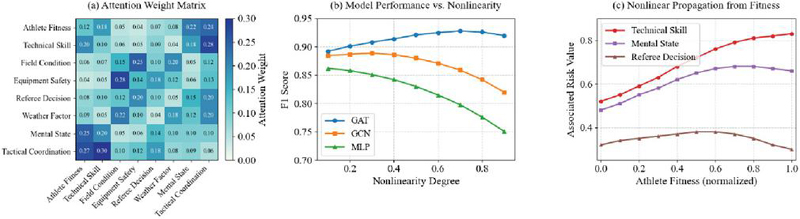
Figure 7 Analysis of complex risk relationship modeling capability: (a) heatmap of attention weights for risk factors, (b) comparison of F1 scores for different models under different degrees of nonlinearity, and (c) nonlinear propagation curves of physical fitness factors on related factors.
In Figure 7(a), the horizontal axis represents the neighbor node numbers and the vertical axis represents the attention weights of node 0 to each neighbor. Node 0 has a weight of 0.45 for neighbor 1, 0.20 for neighbor 2, 0.15 for neighbor 3, 0.12 for neighbor 4, and 0.08 for neighbor 5. The attention weights decrease as the neighbor numbers increase, indicating a stronger semantic association between node 0 and neighbors with smaller numbers. This distribution stems from the graph attention mechanism’s adaptive weight calculation based on the feature similarity between nodes, allowing neighbors semantically closer to the central node to receive a higher contribution to information propagation. In Figure 7(b), the horizontal axis represents the propagation rounds, and the vertical axis represents the cosine similarity between the node representation and the global average representation. Node A increases from 0.62 to 0.89, node B from 0.55 to 0.81, and node C from 0.48 to 0.77. The similarity of all nodes increases monotonically with the propagation rounds, indicating that message passing in the graph structure gradually aggregates neighborhood information to the node representation, causing node features to converge towards the global semantic center. Node C has the lowest initial similarity, but its absolute growth rate of 0.29 is higher than that of node A (0.27), reflecting that the attention mechanism exerts a stronger correction effect on nodes with larger initial semantic offsets. In Figure 7(c), the horizontal axis represents the propagation rounds, and the vertical axis represents the node classification accuracy. The accuracy increased from 0.72 to 0.92 under the multi-head attention configuration, from 0.68 to 0.86 under single-head attention, and from 0.60 to 0.70 under the no-attention configuration. Multi-head attention significantly outperforms single-head attention in all rounds, and the latter outperforms the no-attention configuration, indicating that multi-head attention captures different semantic relationships in parallel across multiple subspaces, improving the completeness of information propagation and node classification performance. The no-attention configuration uses a simple neighborhood average, losing the importance differences between nodes, and therefore has the lowest propagation efficiency. Combining the three subgraphs, it can be seen that the graph attention mechanism can effectively construct non-uniform semantic propagation paths, accelerate the semantic alignment of node representations, and improve the performance of downstream classification tasks.
4.4 Analysis of the Effect of Semantic Consistency Optimization
To verify the optimization effect of the contrastive learning mechanism on the semantic space distribution, the contrastive loss value was recorded after every five rounds during model training. At the same time, the cosine similarity of positive and negative sample pairs was collected, and high-dimensional features before and after contrastive learning were extracted for t-SNE dimensionality reduction and visualization, thus obtaining the semantic consistency optimization effect analysis diagram shown in Figure 8.
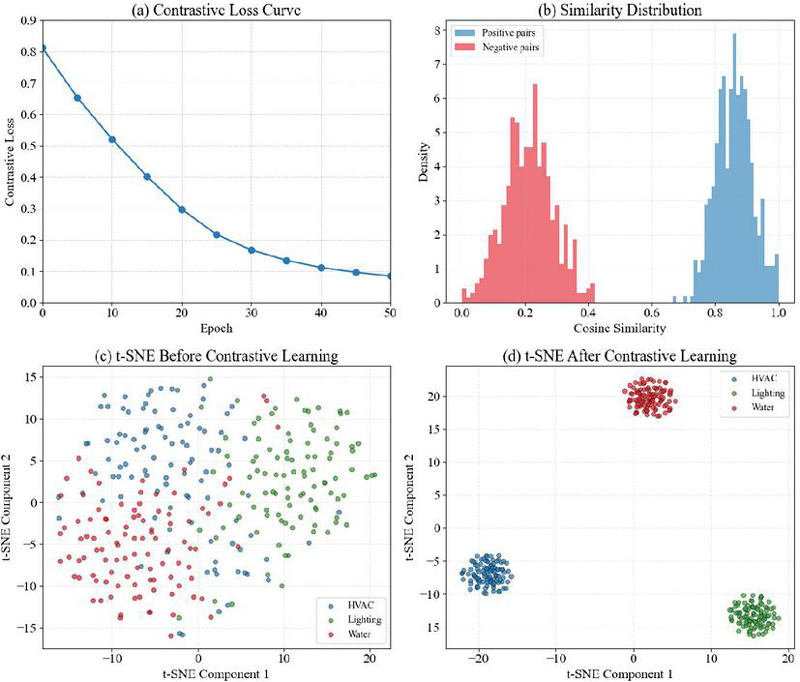
Figure 8 Analysis of the effect of semantic consistency optimization: (a) contrast loss curve, (b) similarity distribution, (c) comparison of the SNE distribution before learning t, and (d) comparison of t-SNE distributions after learning.
Figure 8 contains four sub-figures, comprehensively demonstrating the promoting effect of contrastive learning on semantic space convergence. Figure 8(a) shows the training epochs on the horizontal axis and the contrastive loss value on the vertical axis. The loss value decreased from 0.812 in epoch 0 to 0.085 in epoch 50, a cumulative reduction of 0.727. This continuous downward trend indicates that the contrastive loss function was effectively optimized during training, and the model gradually narrowed the representation distance between semantically similar samples. The reason for this phenomenon is that gradient descent updates continuously adjust the encoder parameters, enhancing the discriminative ability of positive and negative sample pairs. Figure 8(b) presents the cosine similarity distribution of positive and negative sample pairs as a histogram. The similarity of positive sample pairs is concentrated in the interval between 0.85 and 0.90, while that of negative sample pairs is concentrated in the interval between 0.15 and 0.25, with almost no overlap between the two distributions. This separation indicates that contrastive learning successfully clustered similar data and pushed apart dissimilar data, forming a clear semantic boundary. This is because the contrastive loss function simultaneously imposes constraints to bring positive sample pairs closer and push negative sample pairs further apart, forcing the encoder to extract common features related to device categories. Figure 8(c) shows the dimensionality reduction results of high-dimensional features for HVAC, lighting, and water systems before contrastive learning. The sample points show severe overlap, with different categories mixed in multiple regions and unclear class boundaries. This indicates significant semantic fragmentation in the original multi-source heterogeneous data, with similar devices scattered throughout the feature space due to differences in sensor sources. This phenomenon arises because the original features were directly concatenated without semantic alignment, resulting in inconsistent distributions of data from different modalities. Figure 8(d) shows the feature distribution after contrastive learning. The three types of samples form three separate clusters, each highly compact with clear intervals between clusters. HVAC samples are concentrated in the lower left region, lighting samples in the right region, and water system samples in the upper left region. This distribution demonstrates that the contrastive learning constraint effectively corrects the semantic space, causing the representation of similar data to converge to a narrow region. This is because contrastive learning forces the model to ignore irrelevant modal differences such as sensor type and sampling frequency, focusing instead on semantic information related to device function. In summary, the contrastive learning mechanism significantly improves the semantic consistency of cross-system data chains, providing an aligned and compact feature foundation for upper-level decision analysis.
4.5 Decision Response Performance Analysis
To evaluate the response performance of the proposed model in the decision support phase, this study designed three complementary tests: recording the average latency change through an incremental concurrent request load, characterizing the overall distribution characteristics of response latency through cumulative latency distribution, and monitoring the system’s operational stability through continuous 60-second latency sampling under a fixed load. Based on the above test results, the comprehensive decision response performance diagram shown in Figure 9 is plotted.
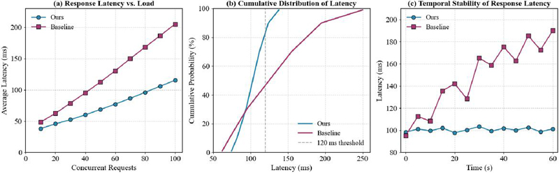
Figure 9 Decision response performance analysis: (a) load-delay response curve, (b) delay cumulative distribution curve, and (c) response delay time stability curve.
In Figure 9(a), the horizontal axis represents the number of concurrent requests and the vertical axis represents the average response latency. The circular curve represents the proposed method, and the square curve represents the baseline method. When the number of concurrent requests increases from 10 to 100, the average latency of the proposed method increases from 38.2 milliseconds to 115.3 milliseconds, consistently lower than the baseline method’s 48.5 milliseconds to 205.1 milliseconds. This data indicates that the latency growth of the proposed method is more gradual under high load. This is because cross-modal semantic alignment and graph attention mechanisms reduce redundant computation in the data preprocessing stage, enabling the decision module to obtain a unified feature representation more quickly. In Figure 9(b), the horizontal axis represents the latency value and the vertical axis represents the cumulative probability. The two curves correspond to the latency distribution of the two methods, respectively. The proposed method has a latency of 124 milliseconds at the 90th percentile, while the baseline method reaches 125 milliseconds at the 50th percentile. The proposed method increases the proportion of responses within 120 milliseconds to approximately 90%. This distributional advantage stems from the fact that the contrastive learning constraint compresses the representation distance of semantically similar nodes, reducing outlier retrieval time in the feature space. Figure 9(c) shows the horizontal axis as runtime (seconds) and the vertical axis as instantaneous latency. The circular curve represents the proposed method, and the square curve represents the baseline method. Within a 60-second monitoring window, the latency fluctuation range of the proposed method remained between 97.8 ms and 103.5 ms, with a standard deviation of only 1.8 ms, while the latency of the baseline method continuously climbed from 95.2 ms to 190.1 ms with significant fluctuations. This difference in stability reflects that the proposed method eliminates dynamic latency jitter caused by cross-system data format conversion through a unified semantic embedding space. Combining the test results of the three subgraphs, the proposed method significantly outperforms the baseline method in terms of mean, distribution, and temporal stability of response latency.
5 Conclusions
This paper addresses the problem of semantic fragmentation in multi-source heterogeneous data for sustainable sports facility management. To this end, it develops a GNN framework for cross-modal semantic alignment, in which raw IoT data are mapped into a shared embedding space through a unified encoding function. A heterogeneous graph structure is then constructed by integrating device topology with functional coupling relationships, and weighted propagation of node features is performed under the guidance of a graph attention mechanism. In addition, contrastive learning constraints are introduced to optimize the distribution of the semantic space, thereby generating a semantically consistent feature representation that can be effectively incorporated into the decision-support process. Experimental results demonstrate substantial improvements across several key indicators: interoperability consistency increased from 0.52 to 0.89, cumulative probability at an error threshold of 0.2 rose from 0.30 to 0.82, and semantic alignment accuracy reached 92.4%. These results confirm the effectiveness of the proposed method in semantic fusion and structural relationship modeling. Overall, the study shows that the proposed framework enables unified data-chain representation and high-quality semantic alignment in complex IoT environments, thereby providing a reliable data foundation for facility operation assessment and resource scheduling, with strong practical value for green, low-carbon, and intelligent operation and maintenance.
Conflict of Interest
The authors declare that there is no conflict of interest regarding the publication of this paper.
References
[1] Bibri, Simon Elias, et al. Environmentally sustainable smart cities and their converging AI, IoT, and big data technologies and solutions: an integrated approach to an extensive literature review. Energy informatics 6.1 (2023): 9.
[2] Mrabet, Manel, and Maha Sliti. Integrating machine learning for the sustainable development of smart cities. Frontiers in Sustainable Cities 6 (2024): 1449404.
[3] Zhang, Wen, Lingling Li, and Yu Li. Natural Ventilation and Energy Consumption Research for Dry Sports Halls Within National Fitness Centers in Cold Regions–Case Study of Qingdao. Buildings 15.5 (2025): 734.
[4] Almaleck, Pablo, et al. Electrical consumption forecasting in sports venues: A proposed approach based on neural networks and ARIMAX Models. Sustainable Cities and Society 100 (2024): 105019.
[5] Cheng, Mingkai, and Wu Lv. IoT-Driven Community Sports Management: Machine Learning for Data Processing. Journal of Advanced Computational Intelligence and Intelligent Informatics 30.2 (2026): 372–387.
[6] Hu, Yang, et al. Internet of Things enabled deep learning monitoring system for realtime performance metrics and athlete feedback in college sports. Scientific Reports 15.1 (2025): 28405.
[7] Zhao, Hairu. Intelligent management of industrial building energy saving based on artificial intelligence. Sustainable Energy Technologies and Assessments 56 (2023): 103087.
[8] Selvaraj, Rajalakshmi, Venu Madhav Kuthadi, and S. Baskar. Smart building energy management and monitoring system based on artificial intelligence in smart city. Sustainable Energy Technologies and Assessments 56 (2023): 103090.
[9] Gregori-Faus, Cristian, et al. State-of-the-art of sustainability in sports facilities: a systematic review. Environment, Development and Sustainability (2025): 1–22.
[10] Wang, Yuchen, and Lu Liu. Research on sustainable green building space design model integrating IoT technology. PloS One 19.4 (2024): e0298982.
[11] Alsabah, Muntadher, et al. A comprehensive review on key technologies toward smart healthcare systems based IoT: technical aspects, challenges and future directions. Artificial Intelligence Review 58.11 (2025): 343.
[12] Kayvanfar, Vahid, et al. A review of decision support systems in the Internet of Things and supply chain and logistics using web content mining. Supply Chain Analytics 6 (2024): 100063.
[13] Ranpara, Ripal. A semantic and ontology-based framework for enhancing interoperability and automation in IoT systems. Discover Internet of Things 5.1 (2025): 22.
[14] Marshoodulla, Syeda Zeenat, and Goutam Saha. An approach towards removal of data heterogeneity in SDN-based IoT framework. Internet of Things 22 (2023): 100763.
[15] Liu, Xiufeng, et al. IoT-enabled interoperability for energy-mobility integration: A systematic review of protocols, platforms, and standards. Applied Energy 411 (2026): 127611.
[16] Ait Abdelouahid, Rachida, et al. Literature review: clinical data interoperability models. Information 14.7 (2023): 364.
[17] Zhu, Min, et al. An intelligent collaboration framework of IoT applications based on event logic graph. Future Generation Computer Systems 137 (2022): 31–41.
[18] Domínguez-Bolaño, Tomás, et al. An IoT system for a smart campus: Challenges and solutions illustrated over several real-world use cases. Internet of Things 25 (2024): 101099.
[19] Varalakshmi, K, and J Kumar. Optimized predictive maintenance for streaming data in industrial IoT networks using deep reinforcement learning and ensemble techniques. Scientific Reports 15.1 (2025): 27201.
[20] Kaur, Kawalpreet, et al. Unveiling the core of IoT: comprehensive review on data security challenges and mitigation strategies. Frontiers in Computer Science 6 (2024): 1420680.
[21] Xu, Kan, et al. Semantic model-based large-scale deployment of AI-driven building management applications. Automation in Construction 165 (2024): 105579.
[22] Farahani, Bahar, and Amin Karimi Monsefi. Smart and collaborative industrial IoT: A federated learning and data space approach. Digital Communications and Networks 9.2 (2023): 436–447.
[23] Elhajj, Mohammed. Semantic Foundations for Digital Twins: The Contribution of Ontological Analysis. Frontiers in Computer Science 8: 1757450.
[24] Acharya, Sarthak, et al. Empirical insights on interoperability in digital twins: Challenges & LCIM perspectives. Information and Software Technology (2026): 108048.
[25] Natarajan, Yuvaraj, et al. Enhancing building energy efficiency with IoT-driven hybrid deep learning models for accurate energy consumption prediction. Sustainability 16.5 (2024): 1925.
[26] Liang, Zheng, and Junjie Chen. Research on building energy consumption prediction algorithm based on customized deep learning model. Energy Informatics 8.1 (2025): 25.
[27] Huang, Xiongwei, et al. BIM and IoT data fusion: The data process model perspective. Automation in Construction 149 (2023): 104792.
[28] Fatemi, Narges, and Javad Fattahi. Adaptable semantic interoperability in heterogeneous smart grids using Large Language Models. Energy Reports 14 (2025): 5774–5789.
[29] Vijaya, Annas, et al. From fragmentation to interoperability: How semantic models transform environmental, social, governance (ESG) reporting, knowledge, and sustainability governance. Journal of Innovation & Knowledge 13 (2026): 100924.
[30] Vittori, Filippo, et al. BIM-to-BRICK: Using graph modeling for IoT/BMS and spatial semantic data interoperability within digital data models of buildings. Energy and Buildings (2025): 116368.
Biographies

Rui Zhang is a Lecturer in Physical Education at Anhui Vocational College of Defense Technology, Lu’an, China. He received his postgraduate degree. His research interests include tennis teaching and physical training.

Yang Jiang is an Associate Professor in Physical Education at Anhui Sports Vocational and Technical College, Hefei, China. He received his postgraduate degree. His research interest focuses on physical training.
Journal of ICT Standardization, Vol. 14_3, 311–338
doi: 10.13052/jicts2245-800X.1432
© 2026 River Publishers