Load Passenger Forecasting Towards Future Bus Transportation Network

Clément Vial^1,* and Vivien Gazeau^2,*

¹Alstom Digital Mobility, Villeurbanne, France

²RATP Group – Régie Autonome des Transports Parisiens, Paris, France

Email: clement.vial@alstomgroup.com; vivien.gazeau@ratp.fr

* Corresponding Author

Received 11 July 2019; Accepted 16 October 2019; Publication 18 July 2020

Abstract

Knowing the load of a transport system is one of the critical information of the operators and allows them to take strategic moves to optimize the line, involving more buses or changing the missions of the buses. Having this information in real-time and in the near future opens a new dimension in the management possibilities of the line. The paper describes a prototype that demonstrates this possibility and exposes the methodology used and some examples of the results. The study here presented was possible thanks to a new kind of data: the counting of passengers boarding and dropping out at each stop provide by sensors installed above the doors.

Keywords: Smart cities, IoT, urban transportation, load passenger forecast, bus intelligent network.

1 Introduction

Work focusing on prediction of bus arrival exists for some years now, with a renewed interest thanks to new data available and more performant algorithms. Thanks to the new kind of sensors installed on buses, the methods usually use GPS track to study their speed and associated patterns.

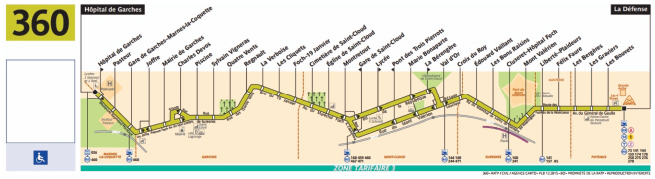
Figure 1

However, bus passenger load prediction is another story. Historic bus position is already known with a significant time window, and more recently, Automatic Fare Collection (AFC) provided not only validation data for the whole line but also anonymous user information with position and timestamp.

Those validation data allow to know with an excellent precision how many people board the buses for each stop and each time, with the following limitations: people that don’t have ticket (fraud), or systems with different ticket supports that are not recorded the same way (in this use case, the validation data of the smart cards are available, but not the magnetic tickets). (Lathia et al., 2012)

The main limitation is that this data doesn’t provide the information about the passengers dropping out: there is only half of the new information.

Some studies have used the smart card data to try to build the passenger trip pattern of some passengers (where the passenger validates in the morning, and then at the end of the day can give a clue about where he usually drops out) and build a probabilistic model for the missing passengers. However, this needs to be checked against Origin-Destination matrices made from field studies and polls.

This study is focused on a dedicated bus line in the Paris neighborhood. This study is part of MSM project (Modeling of Mobility solution) which involves Alstom, RATP and IRT SystemX (Technologic Research Institute)

This line is already equipped with passenger counting solutions for onboarding and dropping off passengers. Onboard sensors have been updated to provide information in Realtime.

Line 360 starts in La Défense district (which is connected to a mass transit system: Suburbans train, regional trains, metro, tramway, and buses) and lasts in Hôpital de Garches, in the west of Paris.

Some other stops of the line are also connected to suburban train lines, but they are smaller lines than La Défense.

Those sensors reconstruct a 3D map of the environment by recording the flight time of the infrared rays. Then, they detect the heads and shoulder to localize the persons, then track them to see if they cross some successive virtual lines and count one if they are all crossed successively.

Recording starts when the bus comes near a stop (about 40m), and when the bus leaves the station (closing of the doors and releasing of the brakes). In this way, it is possible to know the quantity of people onboarding and dropping out of the bus at each stop.

The counting data contains the following fields:

Direction
Stop name
Bus identifier
Quantity of onboarding
Quantity of dropping out

However, the GPS signal is not always reliable in cities because of their reflections on the walls of the buildings or their absorption. This leads to some stops or direction errors in the data are erroneous, and an essential work of corrections had to be done.

2 Data Collection

RATP is the leading Public Transport Operator in Greater Paris Area. The 4700 bus fleet is already equipped with different technologies of sensors for automated Passenger Counting (APC). Most of the fleet uses infrared sensors to count the number of passengers getting off the bus. This sensor has an accuracy of 70% to 80% and was installed during the 90s to the 2000s. The number of boarding passengers was reconstructed with the number of validations which allowed to have an idea of the passenger load.

Since 2010, new sensors using CMOS 3D technology are offered by suppliers. This new generation of sensors is installed above the doors when buses are renewed. They detect a pattern of head and shoulders at 1m from the ground, which corresponds to people over four years old, and has an accuracy of 98%.

At the end of each day, when the buses come back to the bus depot, data are transferred from each bus through a Wi-Fi connection and gathered in a central system for processing and reporting.

In this study, the aim to better understand people’s behavior and adapt the transport offer to the transport demand in real-time. The decision has been made to choose to study bus line 360, a line in the west of Paris, which goes from La Défense – a business district – to Garches’ Hospital. This bus line encounters difficulties and frequent delays. Ten buses of the same model make up the fleet for this line. In order to send the passengers’ count in real-time after each stop point and to avoid any disagreement with the legacy counting system, the buses wiring have been retrofitted. Data are sent to cloud storage. Each batch of data sends the following items: GPS location, Operating Device Time, bus line ID, bus ID, missions ID, stop ID, Number of passengers IN, Number of passengers OUT. Those ten buses are now IoT devices, and the information system is set up.

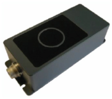
Figure 2 SIRA3D sensor.

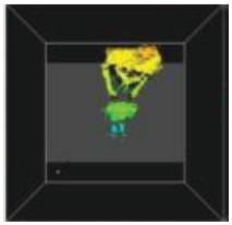
Figure 3 Snapshot from the sensor.

3 Reconstruction of the Load

The load is calculated using the number of people boarding and dropping out of the bus at each stop and integrating using assumptions on initial amounts. At La Défense, the initial load before the first count is 0, and at Hôpital de Garches in the return direction, the value of the capacity of the preceding stop is kept. Indeed, an important quantity of passengers onboarding the bus at the last stop of the outward direction to have some sited place in the return direction. However, this reconstruction of the load is based on another reconstructed data: the trip of the bus.

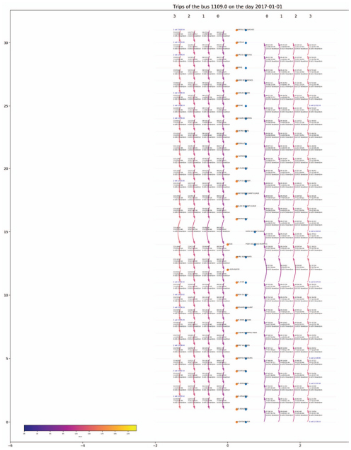
Figure 4 Chart terminuses.

The difficulty here is that a bus can have different missions, commanded by the operator: for example, in case of high demand at the end of the line in the return direction, the operator will control the buses to change course in the middle of the line to increase the transport offer locally.

But the principal difficulty is that the errors on direction or stop caused by an erroneous GPS signal break the logic of the sequence of stops, and it is not possible anymore to perform a correct integration of the boarding and dropping out data. This is why the correction of the errors is mandatory before the reconstruction of the load.

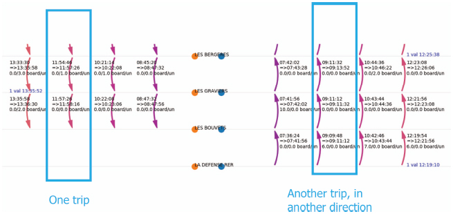
Figure 5 Example of error patterns.

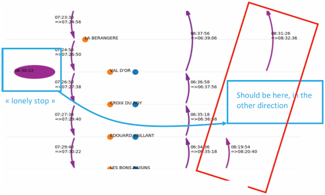
Figure 6 Corrected trip.

To detect the error patterns, and visualize the data, a graphic tool has been created. It shows all the stops reached by bus for a whole day and the associated time. This visualization is augmented by additional information like ticketing data on smart card validation. The stops are displayed vertically at the middle, one direction on the right, and the other on the left. The arrows represent the trajectory of the bus, and their color changes with the hour of the day.

On each arrow, there is the time at which the bus left the last stop, the time at which the bus arrived at the next stop, and the quantity of people onboarding and dropping out.

Here is an example:

This example shows that there is no data at both terminuses for an unknown reason. However, at the beginning of the direction R, the people dropping out should have dropped out at the end of the outward direction, it makes no sense to wait for 15 minutes to drop out at almost the same place. This is why the dropping out data of the first stop of the backward direction have been moved to the last stop of the outward course.

The same visualization with a zoom:

Example of error patterns: There is only one stop on a trip. This is due to an error in the direction.

Once the pattern has been found in the data, the stop is corrected, and the trips are calculated once more. However, this method is not sufficient to adjust the vast quantity of errors in the direction of the stops: the instructions had to be recalculated from scratch, according to the definition of the line and the sequence of stops performed by the bus.

4 Predictive Analysis

4.1 Modeling methods

Successful applications of short-term and long-term passenger load forecasting have already been performed and are available in the literature (Toqué et al., 2017). The short-term predictions focus on the events within a time range of a few hours (useful to manage the buses and the drivers necessary to attend the demand) when the long-term predictions focus on the order of a year (useful to reconsider the sizing of the fleet and the definition of the line).

For the short-term approach, the methods historically used are the historical average, the smoothing techniques, an autoregressive integrated moving average (ARIMA). Since 1970, ARIMA has been quite successful, and seasonal ARIMA models have been developed to further improve its performance (Teng & Shen, 2015). Other methods have also been used, like neural networks, non-parametric regression, Kalman filtering models, and Gaussian maximum likelihood (Xue et al., 2015).

Neural networks have frequently been chosen for their ability to deal with complex non-linear problems without a priori knowledge regarding the relationships between input and output variables. The random forest has also been used, mainly because it is easy to understand how the algorithm works easy to interpret and offers meaningful insights about the problem.

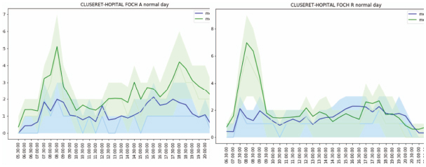
Figure 7 Corrected trip.

There are two possibilities to study the data: focus on the buses or focus on the stops. For this study, the choice is to concentrate on stops as all the coaches have the same configuration and as the operator is more interested in the line than in particular buses, and as there are sensors installed in a few of them counting the passengers, which will allow making some comparisons.

The average behavior of the stops during a typical day (during the week, out of holydays) shows the two main frequentation pics, in the morning around 8, and in the evening around 18h30. However, the number of passengers and the relative importance of those two pics differ quite a lot between two stops. In the pictures under, there is the average number of people boarding and dropping out, and also the first and the third quartiles to have an idea of the variance.

In those examples, there are always more people dropping out than boarding. One could think that this is due to an error in the sensors, but the precedent image showing the repartition of the load in the buses at the end of a round trip shows that in general the sensors count more people than they should in average. Another possibility is that this is the real behavior of the people: they use the bus only for one of their two daily trips. The transport offer in the area is quite essential, as there are several connections to mass transit lines, the users have more options for their commuting routes.

For example, for Liberté-Plaideurs in direction A, the people seem to use the bus to go there at the end of the day, but they don’t seem to use the bus in the morning. In conclusion, it is evident that each stop (one stop per direction) have its behavior, and that a separate model will have to be created for each one.

4.2 Forecasting

For this prediction, the decision has been made to start with the Random Forest algorithm, because

it is easy to use (no need to rescale or transform the data, and can handle binary features, categorical features, and numerical features)
it is parallelizable, so it can smoothly be run on machines with more CPUs if the data to process are huge
it is well adapted to a significant number of features because it works on subsets of data
it is quick for learning and prediction
Low bias and moderate variance
Each decision tree has a high variance, but low bias. But because all the trees are averaged in random forest, the variance is averaged as well so that the result is a low bias and moderate variance model.
It provides a dedicated weight per feature in the model, which is a reasonable basis for interpretation

The features are composed of

Temporal information (hour, day, month, holiday, bridging day, weekend)
History of this stop for boarding, dropping out, load
History of other stops for boarding, dropping out, load
The time delay between the buses

The learning process is composed of two main phases: optimize and learn.

4.3 Optimize

The goal of this phase is to find the parameters that offer the best prediction scores on a test set. The parameters specify the number of trees, but they are also used to determine the creation of the features (for example, the historical time window for a dedicated station). The model is then trained on the part of the dataset (the training dataset) and evaluated by another element, the test set, which represents 50% of the training dataset size. Several methods exist for the creation of the train/test data sets, for example the cross-validation and the rolling windows.

Rolling window takes data from the beginning of the dataset t0 until a date t1 to create the training dataset, and then the data from t1 to t2 to generate a test dataset. Then, another pair of datasets are created with the parameters t0, t1+delta, t2+delta. The cross-validation takes data randomly from the initial dataset and split them into train and test datasets.

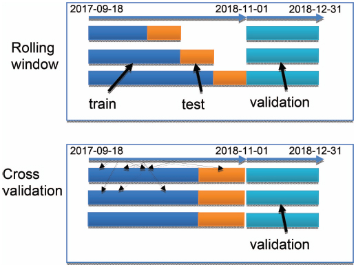
Figure 8 Rolling window.

However, the problem with the cross-validation is that the time series is broken because the order of the elements of the dataset is lost, which represents a lot of information.

Therefore, only the rolling window method is used.

4.4 Learn

The model has learned again with the optimized parameters on the validation dataset. A dedicated dataset different from the train and test datasets is used to avoid using data that influenced the creation of the model. The temporal features are the most important, because the activity of the transport systems is dependent on people’s actions, and they are mainly cyclic (daily routine, yearly holidays . . . ).

The short-term history of this stop can also give a clue on the near-term forecast for passenger demand: for example, if between 6am and 7am more people have been boarding than usual, one can think that at 7:15am there will be more people boarding than usual. There could also be the case where the passengers left earlier (because of a heatwave, for example), but as the global quantity of passengers is still the same, this means that the next buses, which are generally full, will contain fewer passengers. But the past behavior of the other stops is also essential, because for example if the bus is already full, fewer people will board it in the current stop.

5 Estimation and Predictive Models

The load is a complex combination between the past loads/boarding number/dropping out number of this bus on all the preceding stations, and the future boarding/dropping outnumber at the next stop.

The system to be modelized is theoretically more straightforward when restricted to:

– the last load of the bus that will arrive at the stop to be predicted,
– the prediction of the boarding number
– the prediction of the dropping outnumber

And then calculate the load.

The interest of this method is that the boarding and dropping outnumber depend mainly on the activities of the people leaving near this stop, and the value of the prediction depends on fewer parameters.

But the results did not confirm the assumption:

An R² close to one fits quite well the real values, whereas the negative value shows a model that performs worst than a simple constant model. The model for the load of Cluseret-Foch has an excellent performance, whereas the models for the boarding and dropping out passengers are unreliable.

Extracts of predictions for the station Cluseret-Foch:

Blue: prediction

Orange: real values

The boarding and dropping out data have a lot of pics and 0 values, and the algorithm has difficulties in sticking to it.

Table 1

Model	R²
CLUSERET-HOPITAL FOCH_A/boarding	0.059740
CLUSERET-HOPITAL FOCH_A/bus_load	0.953227
CLUSERET-HOPITAL FOCH_A/unboarding	0.222666

Table 2

Station	Target	rmse	Score	Wape
CLUSERET-HOPITAL FOCH_A	bus_load	1,66	0,91	14,68
CLUSERET-HOPITAL FOCH_R	bus_load	3,28	0,89	22,79

Figure 9 Quantity of boarding passengers.

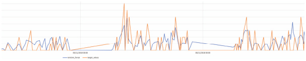
Figure 10 Quantity of passengers dropping out.

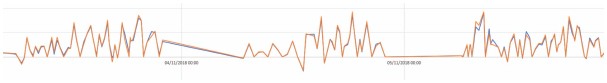
Figure 11 Load of the bus.

The load is also quite irregular, but the algorithm is quite successful in modeling it.

6 Conclusion

The transport operators have a great interest in knowing in depth the behavior of their systems, to see the relevance of their offer and the satisfaction of their clients, but also to optimize them. One of the leading indicators of demand is the passenger bus load. However, this information was not accessible until now.

New sensors installed in the buses counting the quantity of passengers boarding and dropping out paved the way for the reconstruction of the load provided the data can be effectively cleaned. Indeed, the geolocalization system introduced some errors in the dataset, which breaks the logic of the stops sequence of the line, and the reconstitution of the load cannot be done through a simple integration on the flow of passengers on the bus.

This work demonstrated the feasibility of a reliable prediction of the passenger bus load on a stop of the line using the Random Forest algorithm and appropriate features and will be the basis for future developments.

Those future developments will include an integrated system that will provide a real-time data flow of the counting data, augmented with additional information that allows to correcting effectively the errors of the geolocalization system.

They will also include a dashboard informing the operator of the status of the line in real- time and its short-term future, using the models already created and embedded in APIs.

References

[1] Lathia, N., Quercia, D., and Crowcroft, J. (2012). The Hidden Image of the City: Sensing Community Well-Being from Urban Mobility. Pervasive Computing.

[2] Teng, J. and Shen, S. (2015). Modified bus passenger flow forecasting model. 15th COTA International Conference of Transportation Professionals.

[3] Toqué, F., Khouadjia, M., Come, E., Trepanier, M., and Oukhellou, L. (2017). Short & long term forecasting of multimodal transport passenger flows with machine learning methods. IEEE.

[4] Xue, R., Sun, D., and Chen, S. (2015). Short-Term Bus Passenger Demand Prediction Based on Time Series Model and Interactive Multiple Model Approach. Discrete Dynamics in Nature and Society.

Biographies

images

Clément Vial graduated from Ecole Centrale Marseille and currently holds the position of data scientist/data engineer in the innovation team of Alstom Transport, and participate in a project created by the IRT SystemX institute. With a profound background in transports, Clément worked for various transport systems like ticketing, road signalling, platform screen doors, Aesthetic Power Supply. He participated during 4 years to the design, construction and testing of the first tramway project exempt of catenary in Brazil (in Rio de Janeiro) with advanced energy management capabilities (seamless transitions between zones with ground power supply and zones in autonomy), and to the design of the Electrical Road System which will allow electrical trucks to charge while driving in motorways. His passion for programming then led him to create a transportation startup in Salvador de Bahia that connects car owners with drivers that can drive them back home when they can’t. He now succeeded to reconcile his two passions, and work on the data produced by these transport systems that he already knows from experience.

images

Vivien Gazeau graduated from ESME Sudria school of Engineering (Paris, France) in 2004. He also holds an MBA from IAE de Paris (Sorbonne University) since 2015. After several years of IT consulting, he joined the RATP Group (the main public transport operator in Paris) in 2010 as a system engineer. In 2016, he participated in RATP’s intrapreneur program and developed a traffic and fraud mapping tool based on the exploitation of massive passenger counting and validation data. Since 2017, as an innovation project manager at RATP, he has been working on the development of a fleet manager for autonomous vehicles in public transport and on connected infrastructure projects serving smart cities.